City, University of London Institutional Repository
Citation:
Pothos, E. M. and Busemeyer, J. R. (2009). A quantum probability explanation for violations of "rational" decision theory. Proceedings of the Royal Society B: Biological Sciences, 276(1665), pp. 2171-2178. doi: 10.1098/rspb.2009.0121This is the unspecified version of the paper.
This version of the publication may differ from the final published
version.
Permanent repository link:
http://openaccess.city.ac.uk/1979/Link to published version:
http://dx.doi.org/10.1098/rspb.2009.0121Copyright and reuse: City Research Online aims to make research
outputs of City, University of London available to a wider audience.
Copyright and Moral Rights remain with the author(s) and/or copyright
holders. URLs from City Research Online may be freely distributed and
linked to.
A quantum probability explanation for violations of
'rational' decision theory
Emmanuel M. Pothos
1and Jerome R. Busemeyer
21. Department of Psychology, Swansea University, Swansea SA2 8PP, UK. Email:
2. Department of Psychology, Indiana University, 10th St., Bloomington, IN 47405, USA. Email:
Word count: 4,555
The work was carried out equally between the two institutions.
Summary
Two experimental tasks in psychology, the two stage gambling game and the prisoner’s dilemma game, show that people violate the sure thing principle of decision theory. These paradoxical findings have resisted explanation by classic decision theory for over a decade. A quantum probability model, based on a Hilbert space representation and Schrödinger’s equation, provides a simple and elegant explanation for this behaviour. The quantum model is compared to an equivalent Markov model and it is shown that the latter is unable to account for violations of the sure thing principle. Accordingly, it is argued that quantum probability provides a better
framework for modelling human decision making.
Cognitive science is concerned with providing formal, computational descriptions for various aspects of cognition. Over the last few decades, several frameworks have been
thoroughly examined, such as formal logic (e.g., Evans, Newstead, & Byrne, 1991), information theory (e.g., Chater, 1999), classical (Bayesian) probability (e.g., Tenenbaum & Griffiths, 2001), neural networks (Rumelhart & McClelland, 1986), and a range of formal, symbolic systems (e.g., Anderson, Matessa, & Lebiere, 1997). Being able to establish an advantage of one
computational approach over another is clearly a fundamental issue for cognitive scientists. Two criteria are needed to achieve this goal: one is to establish a striking empirical finding that provides a strong theoretical challenge, and the second is to provide a rigorous mathematical argument that a theoretical class fails to meet this challenge. This article reviews findings that challenge the classical (Bayesian) probability approach to cognition, and proposes to exchange this with a more generalized (quantum) probability approach.
The empirical challenge is provided by two experimental tasks in decision making, the prisoner’s dilemma and the two-stage gambling task, which have had an enormous influence in cognitive psychology (and economics—there are over 31,000 citations to Tversky’s work, one of the researchers who first studied these tasks; e.g., Shafir & Tversky, 1992; Tversky &
Kahneman, 1983; Tversky & Shafir, 1992). These experimental tasks are important because they show a violation of a fundamental law of classic (Bayesian) probability theory which, when applied to human decision making, is called the ‘sure thing’ principle (Savage, 1954).
principle was tested by Tversky and Shafir (1992) in a simple two-stage gambling experiment: participants were told that they had just played a gamble (even chance to win $200 or lose $100), and then they were asked to choose whether to play the same gamble a second time. In one condition, they knew they won the first play; in a second condition, they knew they lost the first play; and in a third condition, they did not know the outcome. Surprisingly, the results violated the sure thing principle: following a win/ loss, participants chose to play again on 69% / 59% respectively of the trials; but when the outcome was unknown, they only chose to play again on 36% of the trials. This preference reversal was observed at the individual level of analysis with real money at stake.
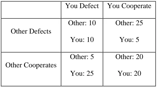
Similar results were obtained using a two person prisoner’s dilemma game with payoffs defined for each player as in Table 1.The Nash equilibrium in standard game theory is for both parties to defect. Three conditions are used to test the sure thing principle: In an ‘unknown’ condition, you act without knowing your opponent’s action; in the ‘known defect’ condition, you know your opponent will defect before you act; and in the ‘known cooperate’ condition, you know your opponent will cooperate before you act. According to the sure thing principle, if you prefer to defect, regardless of whether you know your opponent will defect or cooperate, then you should prefer to defect even when your opponent’s action is unknown.
--- Table 1 ---
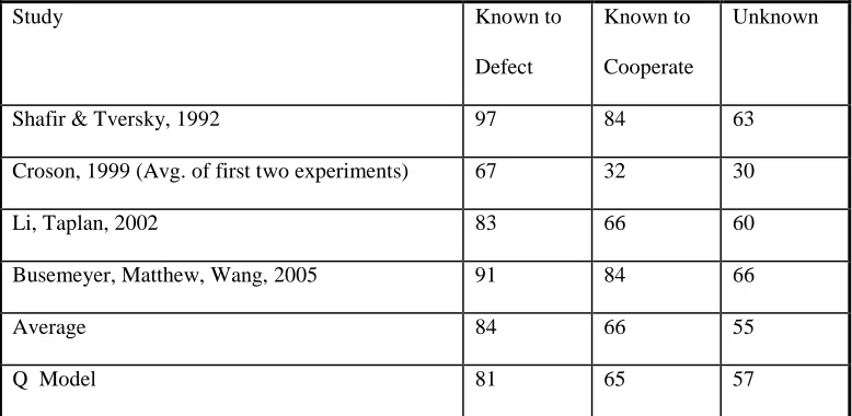
of Shafir and Tversky (1992) has been replicated in several subsequent studies (Busemeyer, Matthew, & Wang, 2006; Croson, 1999; Li & Taplin, 2002, Table 2).
Note that prisoner’s dilemma is a task that has attracted widespread attention not just from decision making scientists. For example, it has been intensely studied in the context of how altruistic and cooperative behaviour can arise in both humans and animals (e.g., Axelrod & Hamilton, 1981; Kefi et al., 2007; Stephens et al., 2002). Violations of the sure thing principle specifically have not been demonstrated in animal cognition. However, both Waite (2001) and Shafir (2001) showed that transitivity, another fundamental aspect of classical probability theory, can be violated in animal preference choice (with gray jays and bees, respectively). Also, it turns out that a core element of our model for human decision making in prisoner’s dilemma has an analogue in animal cognition, raising the possibility that such a model may be applicable to animal cognition as well.
--- Table 2 ---
press) modelled paradoxical results obtained with human probability judgments. Van Rijsbergen (2004; see also Bruza, Widdows, & Wood, 2006; Widdows, 2006) showed that classical logic does not appear the right type of logic when dealing with classes of objects and a more
appropriate representation for classes is possible with mathematical tools from quantum theory. Such approaches can be labelled ‘geometric’ (cf. Aerts & Aerts, 1994) in that they utilize the geometric properties of Hilbert space representations and the measurement principles of quantum theory, but not the dynamical aspects of quantum theory (time evolution with Schrödinger’s equation).
A much smaller number of applications have attempted to apply quantum dynamics to cognition. For example, Atmanspacher, Romer, and Walach (2002) modelled oscillations in human perception of impossible figures. Aerts, Broekaerst and Smets (2004) modelled how a human observer alternates between perceiving the statements in a liar’s paradox situation as false and true. Busemeyer, Wang, and Townsend (2006) presented a quantum model for signal
detection type of human decision processes. Our proposal builds on this latter work (and particularly that of Busemeyer et al., 2006). We were interested in a model which would have implications for the time course of a decision, as well as accurately predicting choice
probabilities in the prisoner’s dilemma and two-stage gambling task. A novel aspect of our proposal is that we attempt to derive a relevant Hamiltonian a priori, on the basis of the psychological parameters of the decision making situation.
brain using quantum mechanics (Hameroff & Penrose, 1996; Pribram, 1993), or developing new algorithms for quantum computation (Nielsen & Chuang, 2000).
The violation of the sure thing principle readily suggests that a classic probability model for Tversky and Shafir’s results will fail. We go beyond intuition and develop a standard Markov model for the two-stage gambling task and prisoner’s dilemma, to prove that this model can never account for the empirical findings. In this way we motivate a more general model, based on quantum probability. Researchers have recently successfully explored applications of the quantum mechanics formalism outside physics (for example, notably computer science. e.g., Grover, 1997). Explorations of how the quantum principles could apply in psychology have been slow, partly because of a confusion of whether such attempts implicate a statement that the operation of the brain is quantum mechanical (e.g., Hameroff & Penrose, 1996). This could be the case or not (cf. Marr, 1982), but it is not the issue at stake: Rather, we are asking whether quantum probability could provide an appropriate mathematical framework for understanding/ modelling certain behavioural aspects of cognition. Key problems in such an endeavour are (a) what is an appropriate Hilbert space representation of the task, (b) what is the psychological motivation for the corresponding Hamiltonian, and (c) what is the meaning of time evolution in this context? We address all these problems in our quantum probability model of decision making in the prisoner’s dilemma task and the two-stage gambling task. The model is described with respect to prisoner’s dilemma task, but extension to the two-stage gambling task is
straightforward.
The prisoner’s dilemma game involves a set of four mutually exclusive and exhaustive outcomes ={BDAD, BDAC, BCAD, BCAC}, where BiAj represents your belief that your
opponent will take the i-th action, but you intend to take the j-th action (D=Defect;
C=Cooperate). For both the Markov and quantum models, we assume that the probabilities of the
four outcomes can be computed from a 4 1 state vector
. For the Markov model,
= Pr[observe belief i and action j], with . For the quantum model, is an
amplitude, so that = Pr[observe belief i and action j], with . For both models, we assume the individual begins the decision process in an uninformed state:
for the Markov model and for the quantum model, .
Step 2: Inferences based on prior information.
Information about the opponent’s action changes the initial state 0 into a new state 1.
If the opponent is known to defect, the state changes to for the Markov model, and
for the quantum model; similarly, if the opponent is known to cooperate, the state
changes to for the Markov model and
for the quantum model. If no
Step 3: Strategies based on payoffs.
The decision maker must evaluate the payoffs in order to select an action, which changes the previous state into a final state We assume that the time evolution of the initial state to the final state corresponds to the thought process leading to a decision.
For the Markov model, we can model this change using a Kolmogorov forward equation
, which has a solution
. The matrix is a transition
matrix, with = Pr[transiting to state i from state j during time period t]. The transition matrix satisfies to guarantee that sums to unity. Initially, we assume
, where
. (1a)
The intensity matrix transforms the state probabilities to favour either defection or
cooperation, depending on the parameters d or c, which correspond to your gain if you defect,
depending on whether you believe the opponent will defect or cooperate, respectively; these parameters depend on the payoffs associated with different actions, and will be considered shortly. The intensity matrix requires Kij > 0 for ij and to guarantee that is a
transition matrix.
For the quantum model, the time evolution is determined by Schrödinger’s equation
with solution . The matrix is unitary with
= Pr[transiting to state i from state j during time period t]. This matrix must satisfy
(identity matrix) to guarantee that retains unit length. Initially, we assume that
The Hamiltonian rotates the state to favor either defection or cooperation, depending on the parameters d or c, which (as before) correspond to your gain if you defect, depending on
whether you believe the opponent will defect or cooperate, respectively. The Hamiltonian must be Hermitian ( ) to guarantee that U is unitary.
For both models, the parameter i is assumed to be a monotonically increasing utility
function of the differences in the payoffs for each of your actions, depending on the opponent’s action: d =u(xDDxDC) and c=u(xCDxCC), where xij is the payoff you receive if your opponent
takes action i and you take action j. For example, given the payoffs in Table 1, uDD = x(10,10),
uDC = x(25,5), uCD = x(5,25), and uCC = x(20,20). Assuming that utility is determined solely by
your own payoffs, then d = u(xDDxDC) = u(5) = = u(xCDxCC) = c. In other words, typically,
i can be set equal to the difference in the payoffs (possibly multiplied by a constant, scaling
factor), although more complex utility functions can be assumed.
For both models, a decision corresponds to a measurement of the state . For the Markov model, Pr[you defect] = Pr[D] = (DD + CD); similarly, for the quantum model, Pr[you
defect ] = Pr[D] = (|DD|2 + |CD|2).
Inserting Equation 1a into the Kolmogorov equation and solving for yields the following probability when the opponent’s action is known:
.
This probability gradually grows monotonically from at t=0 to as t . The behaviour of the quantum model is more complex. Inserting Equation 1b into the Schrödinger equation and solving for yields:
For 1 < < +1, this probability increases across time from at t=0 to at t=1, and subsequently it oscillates between the minimum and maximum values. Empirically, choice probabilities in laboratory-based, decision making tasks monotonically increase across time (for short decision times, see Diederich & Busemeyer, 2006), and so a reasonable approach for fitting the model is to assume that a decision is reached within the interval (0 < t < 1) for the quantum model (t=1 would correspond to around 2s for such tasks).
Equations 1a, 1b produce reasonable choice models when the action of the opponent is known. However, when the opponent’s action is unknown, both models predict that the probability of defection is the average of the two known cases, which fails to explain the violations of the sure thing principle. The KA and HA components of each model can be
understood as the ‘rational’ components of each model, whereby the decision maker is simply assumed to try to maximize utility. In the next section we introduce a component in each model for describing an additional influence in the decision making process, which can lead to
decisions which do not maximize expected utility (and so could lead to violations of the sure thing principle). These two components in each model have to be separate since in many cases the behaviour of decision makers can be explained (just) by an urge to maximize expected utility. The difference between the Markov model and the quantum one relates to how the two
components are combined with each other. Importantly, we prove that the Markov model still cannot produce the violations of the sure thing principle even when this second, non-rational component is added. Only the quantum model explains the result.
To explain violations of the sure thing principle, we introduce the idea of cognitive dissonance (Festinger, 1957). People tend to change their beliefs to be consistent with their actions. In the case of the prisoner dilemma game, this motivates a change of beliefs about what the opponent will do in a direction that is consistent with the person’s intended action. In other words, if a player chooses to cooperate he/ she would tend to think that the other player will cooperate as well. The reduction of cognitive dissonance is an intriguing, and extensively supported, cognitive process. It has been shown with monkeys (Egan, Santos, & Bloom, 2007), suggesting that the applicability of our model might extend to such animals. Shafir and Tversky (1992) explained it in terms of a personal bias for ‘wishful thinking’ and Chater, Vlaev, and Grinberg (2008) by considering a statistical approach based on Simpson’s paradox (specifically, Chater et al. showed that, in a prisoner’s dilemma game, the propensity to cooperate or defect would depend on assumptions about what the opponent would do, given whether the parameters of the game would encourage cooperation or defection). Such approaches may not be
incompatible (for example, wishful thinking may have an underlying statistical explanation). Although cognitive dissonance tendencies can be implemented in both the Markov and the quantum model, we shall see that it does not help the Markov model, and only the quantum model explains the sure thing principle violations.
For the Markov model, an intensity matrix that produces a change of ‘wishful thinking’ is
. (2a)
The first/second matrix changes beliefs about the opponent toward defection/cooperation when you plan to defect/cooperate, respectively.
.
If >1, then the rate of increase for first and last rows is greater than the middle rows, leading to an increase in the probabilities that beliefs and actions agree. For example, setting =10 at t=1
produces
, where it can be seen that beliefs tend to match actions, achieving a
reduction of cognitive dissonance. For the quantum model, a Hamiltonian that produces this change is
. (2b)
The first/second matrix rotates beliefs about the opponent toward defection/cooperation when you plan to defect/cooperate, respectively. Note that
.
If >0, then the rate of increase for the first and last rows is greater than the middle rows, so that, as before, there is an increase in the amplitudes for the states in which beliefs and actions agree. For example, setting =1 at t=/2 produces which results in a vector of squared
magnitudes equal to
. In both the Markov and the quantum model, we can see that the
By itself, Equation 2 is an inadequate description of behaviour in prisoner’s dilemma, because it cannot explain how preferences vary with payoffs. We need to combine Equations 1 and 2 to produce an intensity matrix KC = KA+KB or a Hamiltonian HC = HA+HB so that the time
evolution of the initial state to the final state reflects the influences of both the payoffs and the process of wishful thinking. Note that in this combined model, both beliefs and actions are evolving simultaneously and in parallel.
Accordingly, we suggest that the final state is determined by for the Markov model and for the quantum model. Each model has two free parameters: one changes the actions using Equation 1 and depends on payoffs (i.e., ), and another which corresponds to a psychological bias to assume the opponent will act as we do with Equation 2 (i.e., ).
Model Predictions.
For the Markov model, probabilities for the unknown state can be related to probabilities for the known states by expressing the initial unknown state as a probability mixture of the two initial known states:
.
obeys the law of total probability, which mathematically restricts the unknown state to remain a weighted average of the two known states. Note that this failure of the Markov model occurs even when we include the cognitive dissonance tendencies in the model.
For the quantum model, the amplitudes for the unknown state can also be related to the amplitudes for the two known states:
.
We see that the amplitudes in the unknown case equal the superposition of the amplitudes for the two known cases. However, here is precisely where the quantum model departs from the Markov model: probabilities are obtained from the squared magnitudes of the amplitudes. This last computation produces interference effects that can cause the unknown probabilities to deviate from the average of the known probabilities.
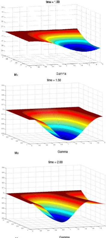
These predictions closely match the observed results (.69, .59, .36, from Tversky & Shafir, 1992). For the prisoner’s dilemma game, setting =.51 and =2.09. produces probabilities for defection equal to (.81, .65, .57) for the (known defect, known cooperate, unknown) conditions, respectively. Again, model predictions closely reproduce the average pattern (.84, .66, .55) in Table 2. Figure 1 shows that model predictions are fairly robust as parameter values vary. An interference effect appears after t=.75 (/2) and is evident across a large section of the parameter space. Finally, note that we can relax the assumption that participants will make a decision at the same time point (we thank a reviewer for this observation). To allow for this possibility, we assumed a gamma distribution of decision times with a range from t = .50(/2) to t=2(/2) and a mode at t=1(/2). We refitted the model using the mean choice probability averaged over this distribution, and this produced very similar predicted results: (.77, .64, .58) for the known defect, known cooperate, and unknown conditions, respectively, in prisoner’s dilemma (with = .47, and = 2.10).
---Figure 1---
Classic probability theory has been widely applied in understanding human choice behaviour. Accordingly, one can naturally wonder whether it is possible to salvage the Markov model. First recall that the classic Markov model fails even when we allow for cognitive dissonance effects in this model. Second, the analyses above hold for any initial state, 0, and
any intensity matrix, K (not just the ones used above to motivate the model), but they are based
marginal probability of defecting in the unknown condition (whatever mixture is used) is a convex combination of the two probabilities conditioned on the known action of the opponent. This prediction is violated in the data of Table 2. Furthermore, even if we change intensity matrices across conditions (using the KA intensity matrix for known conditions and using the KC
matrix for the unknown condition), the Markov model continues to satisfy the law of total probability because this change has absolutely no effect on the predicted probability of defection (the KB matrix does not change the defection rate). Thus our tests of the Markov model are very
robust.
Concluding Comments
In this work we considered empirical results which have been a focal point in the controversy over whether classic probability theory is an appropriate framework for modelling cognition or not. Tversky, Shafir, Kahneman and colleagues have argued that the cognitive system is generally sensitive to environmental statistics, but is also routinely influenced by heuristics and biases which can violate the prescription from probability theory (Tversky & Kahneman, 1983; Tversky & Shafir, 1992; cf. Gigerenzer, 1996). This position has had a massive influence not only in psychology, but also in management sciences and economics, collimating to a Nobel Prize award to Kahneman. Moreover, findings such as the violation of the sure thing principle in Prisoner’s Dilemma has led researchers to raise fundamental questions about the nature of human cognition (for example, what does it mean to be rational? Oaksford & Chater, 1994).
In this work, we adopted a different approach from the heuristics and biases one
be modelled within a probabilistic framework, but classic probability theory is too restrictive to fully describe human cognition. Accordingly, we explored a model based on quantum
probability, which can subsume classic probability, as a special case. The main problems in developing a convincing cognitive quantum probability model are to determine an appropriate Hilbert space and Hamiltonian. We attempted to present a satisfactory prescriptive approach to dealing with these problems and so encourage the development of other quantum probability models in cognitive science. For example, the Hamiltonian is derived directly from the
parameters of the problem (e.g., the payoffs associated with different actions) and known general principles of cognition (e.g., reducing cognitive dissonance). Importantly, our model works: it is able to account for violations of the sure thing principle in prisoner’s dilemma and the two-stage gambling task and leads to close fits to empirical data.
the process collapse onto exactly one preference order. This contrasts with time development in the Markov model, whereby the system monotonically converges to its final state. Third, quantum probability models allow interference effects which can make the probability of the disjunction of two events to be lower than the probability of either event individually (see also Khrennikov, 2004). Such interference effects are ubiquitous in psychology, but incompatible with Markov models, which are constrained by classic probability laws. Fourth, ‘back to back’ measurements on the same decision will produce the same result in a quantum system (because of state reduction), which agrees with what people do (Atmanspacher, Filk, & Romer, 2004). However, ‘back to back’ choices remain probabilistic in classic random utility models, which is not what people do. Finally, recent results in computer science show quantum computation to be fundamentally faster compared to classic computation, for certain problems (Nielsen & Chuang, 2000). Perhaps the success of human cognition can be partly explained by its use of quantum principles.
Electronic supplementary material. Additional proofs.
1. Rational for choice of compatible (commuting observable) over incompatible (non commuting
observable) representation of measurements. .
The prisoner dilemma experiment involves two different types of measurements: one is a
measure of the belief about what an opponent will do (the opponent will defect or cooperate); the second is a measure of the preference for an action to take (decide to defect or cooperate).
According to quantum theory, two measurements can be compatible (commuting observables) or incompatible (non commuting observables). We chose not to treat them as compatible for the following empirical reason. If the two measures are incompatible, then the transition matrix
must be doubly stochastic (Peres, 1995, p. 33 ). This implies that Pr[Defect Action | Cooperate Belief] = Pr[Cooperate action | Defect Belief] = 1 Pr[ Defect action | Defect Belief] which is strongly violated in Table 2. The above transition matrix does not have to be doubly stochastic for the compatible representation.
noncommutativity in preferences and Franco, in press, explains the conjunction fallacy in a similar way).
2. Application of the quantum model to the two stage gambling paradigm.
In this application, we define the four basis states as {|BWAP, |BWAN, |BLAP, |BLAN} where
|BiAj represents the state where you believe that outcome i (W = win, L = lose) occurred on the
previous round, and you choose action j (P = play or N = not play) on the next round. The parameter represents the difference between the expected utility of the gamble and the utility of the sure amount. The parameter rotates the beliefs so that if you plan to play again, then your beliefs rotate toward winning; if you do not plan to play again, then your beliefs rotate toward losing.
3. Proof that the Markov and quantum models predict that the probabilities for the unknown case
are equal to the average of the probabilities for the known cases when only Equations 1a and 1b
are used to generate the final probabilities.
We prove this for the quantum model. The same argument applies for the Markov model. The state after step 3 for the unknown case equals
.
Note that the tensor product separation of the state vector involves a part of what I believe the opponent will do what I intend to do myself. Also, observe that is the state after step 3
given that the opponent is known to defect, and is the state after step 3 given that the opponent is known to cooperate.
In order to compute the probability of me defecting from this state vector, we need to apply the operator
. This operator leaves unchanged the part of the state vector corresponding
to my belief of what the opponent does and collapses the part of the state vector corresponding to my intended action along the eigenstate for defecting. Accordingly, the probability of defecting for the unknown state equals
These two vectors are orthogonal and so
.
The last expression equals the equal weight average of the probability of defecting given the opponent is known to defect ( ) and the probability of defecting given the opponent is
known to cooperate ( ).
4. Proof that the Markov model always fails to explain the violations of the sure thing principle,
no matter what initial state is used for the unknown case and for any intensity matrix.
Define for the Markov model, where K is an arbitrary intensity matrix. Define
to be an arbitrary initial state where
and and and . In the
unknown case, the final state equals
. The two parts, and , determine the probabilities of defection when you know the opponent’s decision. Thus the probability of defection in the unknown case is a weighted average or convex combination of the two known cases with weights equal to p and (1-p).
On the one hand, if the opponent is known to defect, then the state after step 3 equals
;
on the other hand, if the opponent is known to cooperate, then the state after step 3 equals
.
Then for the unknown case, the state after step 3 equals
= .
The probability of defecting in the two known cases equal
The probability of defecting in the unknown case equals
where the last term in soft brackets is the interference term, which is non zero because the two vectors are not orthogonal.
6. Proof that if we use KA for the two known conditions, and we use KC only for the unknown
condition, then the Markov model still obeys the law of total probability and fails to explain the
violations of the sure thing principle.
According to the Markov model, the probability of choosing defection is determined by adding the first and third row of (t) as follows: , where J = [1 0 1 0]. For the unknown condition, this probability changes across time according to the differential equation
,
because JKB = 0 (this is obvious in the expression immediately below Eq 2a). Thus KB has no
effect on this probability. This implies that the probability of defection in the unknown case equals
.
Now we can always define by setting
,
.
Thus if we use only the KA intensity matrix for the known cases, and we use the combined KC
intensity for the unknown case, then this does not change the probabilities of defection and the law of total probability must be maintained. The belief intensity matrix KB only changes the
References
Aerts, D. & Aerts, S. (1994). Applications of quantum statistics in psychological studies of decision processes. Foundations of Science, 1, 85-97.
Aerts, D. & Gabora, L. (2005a). A theory of concepts and their combinations I. Kybernetes, 34, 151-175.
Aerts, D. & Gabora, L. (2005b). A theory of concepts and their combinations II: A Hilbert space representation. Kybernetes, 34, 176-205.
Aerts, D., Broekaert, J., & Gabora, L. (in press). A case for applying an abstracted quantum formalism to cognition. New Ideas in Psychology.
Aerts, D., Broekaerst, J., & Smets, S. (2004). A Quantum structure description of the liar paradox. International Journal of Theoretical Physics, 38, 3231-3239
Anderson, J. R., Matessa, M., & Lebiere, C. (1997). ACT-R: A theory of higher level cognition and its relation to visual attention. Human Computer Interaction, 12, 439-462
Atmanspacher, H., Filk, T., & Romer, H. (2004). Quantum Zeno features of bistable perception. Biological Cybernetics, 90, 33-40.
Atallah, H. E., Frank, M. J., & O’Reilly, R. C. (2004). Hippocampus, cortex, and basal ganglia: Insights from computational models of complementary learning systems. Neurobiology of Learning and Memory, 82, 253-267.
Axelrod, R. & Hamilton, W. D. (1981). The evolution of cooperation. Science, 211, 1390-1396. Bordley, R. F. (1998). Quantum mechanical and human violations of compound probability
principles: Toward a generalized Heisenberg uncertainty principle. Operations Research,
Bruza, P., Widdows, D., & Woods, J. (2007) A quantum logic of down below. In K. Engesser, D. Gabbay, & D. Lehmann (Eds.) Handbook of quantum logic, quantum structures, and quantum computation. Vol 2. Elsevier.
Busemeyer, J. R. , Matthew, M., & Wang, Z. A.(2006). Quantum game theory explanation of disjunction effects. In R. Sun, N. Miyake, Eds. Proceedings of the 28th Annual Conference of the Cognitive Science Society, pp. 131- 135. Mahwah, NJ: Erlbaum.
Chater, N. (1999). The Search for Simplicity: A Fundamental Cognitive Principle? Quarterly Journal of Experimental Psychology, 52A, 273-302.
Chater, N., Vlaev, I., & Grinberg, M. (2008). A new consequence of Simpson’s paradox: stable cooperation in one-shot prisoner’s dilemma from populations of individualistic learners. Journal of Experimental Psychology: General, 137, 403-421.
Croson, R. (1999). The disjunction effect and reason-based choice in games. Organizational Behavior and Human Decision Processes, 80, 118-133.
Diederich, A. & Busemeyer, J. R. (2006). Modeling the effects of payoffs on response bias in a perceptual discrimination task: Threshold bound, drift rate change, or two stage processing hypothesis. Perception and Psychophysics, 97 , 51-72.
Dirac, P.A.M. (1930, 2001) The principles of quantum mechanics. Oxford: Oxford University Press.
Egan, L. C., Santos, L. R. & Bloom, P. (2007). The origins of cognitive dissonance: evidence from children and monkeys. Psychological Science, 18, 978– 983.
Eisert, J., Wilkens, M., & Lewenstein, M. (1999). Quantum games and quantum strategies. Physical Review Letters, 83, 3077-3080.
Festinger, L. (1957). A Theory of Cognitive Dissonance. Stanford Univ. Press, Stanford. Franco, R. (in press). The conjunction fallacy and interference effects. To appear in Journal of
Mathematical Psychology, Special Issue on Quantum Cognition and Decision Making.
Gabora, L., & Aerts, D. (2002). Contextualizing concepts using a mathematical generalization of the quantum formalism. Journal of Experimental and Theoretical Artificial Intelligence, 14, 327-358.
Gigerenzer, G. (1996). Reasoning the fast and frugal way: Models of bounded rationality. Psychological Review, 103, 650-669.
Grover, L. (1997). Quantum mechanics helps in searching for a needle in a haystack. Physical Review Letters, 79, 325.
Haggard, P. & Eimer, M. (1999). On the relation between brain potential and the awareness of voluntary movements. Experimental Brain Research, 126, 128-133.
Hameroff, S. R. & Penrose, R. (1996). Conscious events as orchestrated spacetime selections. Journal of Consciousness Studies, 3, 36-53
Kefi, S., Bonnet, O., & Danchin, E. (2007). Accumulated gain in Prisoner’s Dilemma: which game is carried out by the players? Animal Behaviour, 74, e1-e6.
Khrennikov, A. (2004). Information dynamics in cognitive, psychological, social & anomalous phenomena, in A. van der Merwe, Ed. Fundamental theories of physics, Vol. 138.
Dordrecht, Kluwer Academic Publishers.
La Mura, P. (in press) Projective expected utility. Journal of Mathematical Psychology.
Marr, D. (1982). Vision: a computational investigation into the human representation and processing of visual information. San Francisco: W. H. Freeman.
Mogiliansky, A. L., Zamir, S., & Zwirn, H. (in press) Type indeterminacy: A model of the KT (Kahneman Tversky) - man. To appear in Journal of Mathematical Psychology, Special Issue on Quantum Cognition and Decision Making.
Nielsen, M. A. & Chuang, L. L. (2000). Quantum Computation and Quantum Information. Cambridge, UK: Cambridge University Press.
Oaksford, M. & Chater, N. (1994). A rational analysis of the selection task as optimal data selection. Psychological Review, 101, 608-631.
Pribram, K. H. (1993). Rethinking neural networks: Quantum fields and biological data. Hillsdale, N. J: Earlbaum.
Rumelhart, D. E. & McClelland J. L. (1986). Parallel Distributed Processing, Vol. 1, Foundations. Cambridge, Mass: MIT Press.
Savage, L. J. (1954). The Foundations of Statistics. New York: Wiley.
Shafir, S. (1994) Intransitivity of preferences in honey bees: support for ‘comparative’ evaluation of foraging options. Animal Behavior, 48, 55-67.
Shafir, E. & Tversky, A. (1992). Thinking through uncertainty: nonconsequential reasoning and choice. Cognitive Psychology, 24, 449-474.
Stephens, D. W., McLinn, C. M., & Stevens, J. R. (2002). Discounting and reciprocity in an iterated Prisoner’s Dilemma. Science, 298, 2216-2218.
Tversky, A. & Kahneman, D. (1983). Judgment under uncertainty: heuristics and biases. Science,
185, 1124-1131.
Tversky, A. & Shafir, E. (1992). The disjunction effect in choice under uncertainty. Psychological Science, 3, 305-309.
Van Rijsbergen, C. J. (2004). The Geometry of Information Retrieval. Cambridge UK: Cambridge University Press.
Von Neumann, J. (1932; 1955) Mathematical foundations of quantum theory. Princeton, NJ: Princeton University Press.
Waite, T. (2001) Intransitive preferences in hoarding gray jays (Perisoreus Canadensis). Behavioral Ecology and Sociobiology, 50, 116-121.
Figure captions.
Figure 1. The probability of defection under the unknown condition minus the average for the two known conditions, at six time points (note that time incorporates a factor of pi/2). Negative values (blue) typically indicate an interference effect in the predicted direction.
Table 1. Example payoff matrix for prisoner’s dilemma game.
You Defect You Cooperate
Other Defects
Other: 10 You: 10
Other: 25 You: 5
Other Cooperates
Other: 5 You: 25
Table 2. Empirically observed proportion of defections different conditions in the prisoner’s dilemma game
Study Known to
Defect
Known to
Cooperate
Unknown
Shafir & Tversky, 1992 97 84 63
Croson, 1999 (Avg. of first two experiments) 67 32 30
Li, Taplan, 2002 83 66 60
Busemeyer, Matthew, Wang, 2005 91 84 66
Average 84 66 55
[image:35.612.112.501.234.424.2]SUPPLEMENTARY MATERIAL – ALTERNATIVE PROOFS
3. Proof that the Markov and quantum models predict that the probabilities for the unknown case
are equal to the average of the probabilities for the known cases when only Equations 1a and 1b
are used to generate the final probabilities.
We prove this for the quantum model. The same argument applies for the Markov model. The state after step 3 for the unknown case equals
The above is a direct sum decomposition of the full state space into the state space for Knowing Other D and the state space for Knowing Other C (under all circumstances, this is possible before time evolution).
Ignoring cognitive dissonance, the unitary operator corresponding to the thought process is completely reducible and can be written as a direct sum of its restriction to the subspaces Knowing Other D and Knowing Other C.
So, basically, we have:
.
Note that the initial state vector could be written as
In fact, this formulation is implied in the above equations (highlighted green, from the paper), since the overall state is expressed as a tensor product in this sense:
What is slightly confusing is that, even through the overall state can be written as a tensor product, the operator U *cannot* be written as a tensor product (even in the simple case in which there is no cognitive dissonance). By contrast, the U can be written as a direct sum.
So, this is more a presentation point rather than anything else. Basically, starting from:
We want to reach:
So, as to show that the final (time-evolved) state in the Unknown (general) situation is a convex combination of the final states when the Other D or the Other C.
(When there is no cognitive dissonance.)
My point is that if we recognize that the equation in yellow can be decomposed into a direct sum , then it follows **immediately** that the final, time-evolved state, can also be written as a direct sum .
That is, the additional steps involving the tensor product expression (equation in green) are *not* needed (and have led to some confusion...)
Now, in trying to express the model in more abstract form, we know:
1) Without cognitive dissonance, time evolution can be written as:
. This implies that in the Unknown case, the
amplitudes relating to knowledge that the Other D evolve independently from the amplitudes relating to knowledge that the Other C.
2) Now, with cognitive dissonance we have that
(this is how we constructed ).
3) We also know that with cognitive dissonance the time-evolved state can no longer be written as a direct sum decomposition.
The question is whether we can express these other terms in a more abstract form, although it is not immediately obvious how this can be possible.
Note that the tensor product separation of the state vector involves a part of what I believe the opponent will do what I intend to do myself. Also, observe that is the state after step 3
given that the opponent is known to defect, and is the state after step 3 given that the opponent is known to cooperate.
In order to compute the probability of me defecting from this state vector, we need to apply the operator .
Here we write the state vector as noting that both components
are normalized. Then we have:
The amplitude of this vector is the probability of me D:
But in terms of the computations we make, we can’t separate out the state vector like this:
So, what we do is compute
This operator leaves unchanged the part of the state vector corresponding to my belief of what the opponent does and collapses the part of the state vector corresponding to my intended action along the eigenstate for defecting. Accordingly, the probability of defecting for the unknown state equals
The reason why this is slightly confusing is that you are employing a tensor product operator of the form to a direct sum decomposition of the state vector of the form:
)
.
Note that
and
.
These two vectors are orthogonal and so
.
Then, if I am interested in me D, I need to pick out the relevant state in both subspaces, so that I have to apply the operator (which in itself can be written as a direct sum).
Then,
(where any coefficients are implied in the vectors).
As before, the whole point of avoiding the tensor products is that the general state vector is naturally written as a direct sum of the subspaces for the Other D and the Other C, and the U time evolution operator can be written as a direct sum of its restriction to these subspaces.
The last expression equals the equal weight average of the probability of defecting given the opponent is known to defect ( ) and the probability of defecting given the opponent is known to cooperate ( ).
5. Proof that the quantum model produces interference that violates the law of total probability.
On the one hand, if the opponent is known to defect, then the state after step 3 equals
;
on the other hand, if the opponent is known to cooperate, then the state after step 3 equals
Then for the unknown case, the state after step 3 equals = .
The probability of defecting in the two known cases equal
This demonstration hinges on the fact that and are no longer orthogonal if we allow for cognitive dissonance. As before, I wanted to express this without the tensor product and see whether the resulting formulation might be simpler:
So, *with* cognitive dissonance, we have:
The above can be written as
noting that while the initial state vector could be written as a direct sum, this is *not* the case for the time-evolved state vector and, relatedly, that would in general not be
orthogonal. That is, will have non-zero components for all possible projections.
Then, the probability of me D in the unknown case is given by , which leads to the same result that you obtained. [This will lead to cross terms.]
(Note that without cognitive dissonance the cross terms are of the form:
, whereby and *we know* that , by virtue of fact that these projections exist in different
subspaces.)
The probability of defecting in the unknown case equals
,