The behavior of structures based on the characteristic strain model of creep

The behavior of structures based on the

characteristic strain model of creep

James T Boyle

Department of Mechanical Engineering, University of Strathclyde, Glasgow, Scotland, G1 1XJ

Phone: +441415482311 Fax: +441415525105 E-mail jim.boyle@strath.ac.uk

Abstract There has been much work over the past two decades to aid the design and assessment engineer in the selection of a suitable material model of creep for high temperature applications. The model needs to be simple to implement as well as being able to describe material response over long times. Familiar creep models, as implemented in the majority of nonlinear finite element analysis systems, are still widely used although not always accurate in modeling creep behavior at the end of the secondary phase. The Characteristic Strain Model (CSM) has been shown to be able to effectively model creep behavior at long times; it is simple to implement and requires a

minimum of creep data. This paper examines the ability of the CSM to model the recognized behavior of the steady state creep of simple structures under multi-axial stress.

Keywords Creep – Structural analysis – High temperature design

1 Introduction

creep [1,2,3]. These simplified methods have formed the basis for several high temperature design rules [4,5]. In more recent years the ready availability of nonlinear finite element computational tools has made the use of advanced material models much more accessible, in particular through user material

capabilities as found in software such as ABAQUS. Nevertheless most nonlinear finite element software continue to include the classical time- and strain-

hardening models together with the power law for steady creep amongst several others which have been around for many years. Anecdotal evidence is that these simple models are still widely used for complex finite element design studies. It appears that design engineers continue to prefer simple material models for the analysis of complex, as well as simple, structures.

Part of the work of the ECCC was to provide a source of verified and technically robust creep data for detailed finite element creep analysis and to aid the design engineer in material model selection. A paper by Holdsworth et al [6] examined the issue of the choice of the most appropriate creep model. They investigated the performance of a wide range of creep models on a number of creep datasets - several of these models being modern developments of the classical creep models. No one creep model was identified as having the best performance in terms of representing the creep data over all three stages of creep (primary, secondary and tertiary) with some being more reliable for the primary/secondary stages and some more reliable for tertiary creep, with a few models suitable for both. They

concluded that ‘….. as a generality, it is more important for design and assessment engineers for the model equation to be simple to implement and effective in its description of creep deformation at long times …”. A particular example of such a creep model which satisfied these practical constraints was identified as Bolton’s Characteristic Strain Model [7]. The Characteristic Strain Model (CSM)

much more creep data [6,7]. More recently Bolton [8] has extended the model to include creep recovery (the Duplex Characteristic Strain Model – DCSM). The Characteristic Strain Model is simple to construct mathematically, requires a minimum of creep data and relies on creep rupture data, while being simple enough for the type analytical solutions for simple structures still used by design engineers as well as being suitable for detailed finite element analysis. In a companion paper to [7], Bolton [9] discussed the analysis of structures based on the CSM in a form suitable for design engineers. In this paper, the analysis of structures will be examined to put this new model into the context of conventional creep mechanics.

2 The ‘Characteristic Strain Model’ for creep

2.1 The basic model

The minimum creep rate (_min) during the secondary (or steady state) deformation stage is often related to the (constant) applied stress () by a classical power law relationship in the form

min n B   

(1) where B and n are constants determined from uniaxial creep testing. Use of a power law relation reflects an almost linear relationship between log(minimum creep rate) and log(stress) which is often found in creep tests with the slope being the power exponent n. Typical results for an austenitic stainless steel AISI

lower temperatures (although still above that for creep) even the data from [10] shows similar behavior, Fig.3. Numerous attempts have been made to find a continuous curve to describe this behavior over the complete stress range, principal amongst these being the hyperbolic sine relationship

min Bsinh(C )

   (2) and the combined equation proposed by Garofalo [13]

min sinh( )

n

B C

   (3) where B, C and n are constants. Williams & Wilshire proposed the ‘transition stress’ model [14] for the physical mechanisms associated with power law breakdown

min ( 0)

p B

    (4) where B and p are constants and p is the transition stress. For the transition from

low to moderate stress Naumenko et al [15] proposed a constitutive relationship which assumed that the physical mechanisms were independent and that the corresponding creep rates could simply be added giving a ‘modified power law’:

min

0 0 0

n          _{  }   

 (5)

where 0, 0 and n are material constants. This gives a linear viscous response at low stress and a power law creep response at high stress. The stress 0 is a

different kind of transition stress from that of Williams & Wilshire since it specifies the stress level at which the behavior changes from linear (viscous) with n=1 to power law with a high value of the power exponent, (for example n = 12, Fig. 4). Bolton’s proposed Characteristic Strain Model is much simpler than the models given by eqns.(2)-(5) and makes use of rupture data:

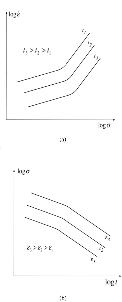
the minimum strain rate during secondary (steady) creep. In the latter, Fig.5(b), contours of constant strain are plotted on a log-log plot of stress versus time. For a given stress level this type of plot would indicate the time at which a given strain was reached; plots of log stress against log time would tend to cluster in tertiary creep as rupture approached indicating the relationship between stress and rupture time. In [7] Bolton argues that the slope of the isochronous curves at low strain tend toward a value of 1, but at high strain the slope tends toward infinity. Then in terms of total creep strain, c, and applied stress, , the slope of the isochronous

curves could be approximated by

(log ) 1

(log ) 1 /

c

R d

d



    (6)

where R is the rupture strength at an appropriate time. This gives a stress

dependent slope for an isochronous curve, varying from n1as  0to n  as  R. For the power law, Eqn.(1), the slope, n, of Eqn.(6) is constant, (log ) (log ) c d n d   

as stress varies.

Integrating Eqn.(6) gives the relationship between creep strain and constant stress at a given time,

/ 1 ch c R     

 (7)

where the integration constant _chis interpreted as a ‘characteristic strain’ inferred to be a material constant at a given time and temperature. In [7] it is shown that

ch

 can be written as

1 ₁ R ch d d        _  _

  (8)

where _R1is the rupture strength at some time t1 (from an isostrain curve,

time t1 ; the latter could be the strain at half the rupture strain as an example.

Further it is shown that _Rcan be approximated as

1 1 1

m

R R

t t

   _{ }

  (9)

where

2 1

1 2

log( / ) log( _R / _R )

t t m

 



and _R2is the rupture strength at time t2. Eqn.(9) assumes that the log-log

isostrain curves in Fig.5(b) can be approximated as a straight line and all have the same slope m. The model is then defined by three constants derived from

available creep data, _R1, _R2and _d.

2.2 A model for steady creep

The basic model, Eqns. (7), (8) & (9), represents a constitutive relation between creep strain, stress and time. In [7] Bolton investigated some properties of the model, while in [9] applied it to two simple structures, a beam in bending and a pressurized thick cylinder, and the finite element analysis of a complex pressure vessel, albeit in a form not typical in creep mechanics. The aim of this paper is to re-examine the use of the model in creep stress analysis and the subsequent behavior of the two simple structures in a more familiar manner. This will be done in the context of nonlinear steady creep:

The Characteristic Strain Model is able to (approximately) represent the secondary stage of creep where a minimum creep rate exists for an extended period for constant stress. Unlike the steady creep rate models from Eqns.(1)-(5) which are based the measured minimum creep rate, the CS model varies

0.2% Creep strength at 100,000 = 75MPa (equivalent to _ch= 0.2%) the variation of creep strain and creep rate with time are plotted in Fig.6. In a study of the characteristics of simple structures it is more convenient to have a version of CSM for steady creep, equivalent to Eqns.(1)-(5) corresponding to the isochronous curve for minimum creep rate against stress, Fig.5(a). Then using the same procedure as Sec.2.1, this would take the form

min

/ 1

ch

R

 

 







 (10)

where, in this case, chand Rcan only be interpreted as material parameters which should, at least in the first instance, have a best-fit to the minimum creep rate/stress isochronous curve, as would be done with the models in Eqns.(1)-(5). For example it is possible to fit Eqn.(10) to the data of Ref.[15], Fig.(4) as shown in Fig.(7) together with the fit for the modified power law,Eqn.(5); the fit is reasonable for low to medium stress but gives much higher strain rates (approaching infinite as expected) for high stress. For low values of stress the characteristic strain model predicts an almost linear variation with stress, as can be seen in Fig.(7). Indeed the model can be interpreted to have a continuously varying slope unlike the power law, Eqn.(1), which would have a constant slope on a log-log plot of creep strain rate against stress.

The steady creep form of the model can then be used to analyze some simple structural components.

3. Simple component behavior

3.1 Pure bending of a beam

The classic problem of the pure bending of a rectangular cross section (bh) beam with a modified power law (stress range dependent constitutive model) subjected to a bending moment M has been considered by Naumenko, Altenbach & Gorash [15] for the modified power law, Eqn.(5). The geometry and loading are as shown in Fig.8. In the following, the notation from [15] is essentially

Under a constant applied bending moment under secondary creep the rate of curvature  of the center-line of the beam is related, assuming pure bending, to the axial (longitudinal) creep strain rate

x z

  (11) where z is measured from the center-line as shown in Fig. 8.

The bending moment is related to the axial stress x through the equilibrium

equation

/2 0

2 h x

M  b



Dimensionless (normalized) variables are defined as

2

2

x

R ch ch

z h

s e e

h                   

Introducing a dimensionless load factor

R M W 



 , where

2 6 bh

W  is the section moment, Eqns. (10), (11) & (12) can be rewritten and combined as:

1 0

( ) 3

e  f s 



Then the rate of change of normalized curvature  can be found, for a prescribed load factor  from a solution of the non-linear equation

1 1 0

3



2

1 1 1

ln(1 )

2 3

 

      (13)

The longitudinal stress distribution s() as it varies with through the thickness  of the beam is then derived from the solution of the non-linear equation

1

( ) ( ) 1/ (1 1/ )

As a reference, for pure power law creep, the solution to Eqns. (13) & (14) corresponds (using the current normalization scheme) to the familiar steady state creep solution for a beam in bending [1, 2, 3]: with

1 1

( ) n

f e e the solution is

2 1 2 1 1/

3 3

n

n

n n

s

n n

 _  _   

 

 (15)

For pure linear (viscous) behavior, the solution is equivalent to that for linear elasticity

   s (16) We can then interpret the load factor  as the ratio of the maximum linear (elastic) stress in the beam to the nominal rupture stressR (without defining what this

means too carefully). Of course both the classic steady state and linear elastic solutions can be normalized such that the normalized curvature rate and longitudinal stress are independent of the load factor .

3.2 Pressurized thick cylinder

The classic problem of a pressurized thick cylinder was also considered by Naumenko, Altenbach & Gorash [15,16] as an example of secondary creep using a modified power law under multi-axial stress. In the following the notation of [15] is repeated, again with minor variations:

Assume that the cylinder is long and uniformly heated, with an inner radius a and an outer radius b, as shown in Fig. 9 and that plane strain conditions prevail. The geometry of the cylinder is best described by a cylindrical polar coordinate system (r,, z); then let the principal strain rates be ( ,    _{r }, _z), the principal stresses be

(  _r, _, _z) and ( )r the von-Mises equivalent stress. The hoop and radial displacement rates are given by vand vrrespectively. The boundary conditions at the inner and outer surfaces are given by

( ) ( ) 0

r a p r b

The solution procedure for this problem is well established [1, 2, 3] and relies on the condition of volume constancy (incompressibility)

, 0 r r r r v dv r dr  

         (18) to reveal that the radial displacement rate has the simple form

r C v

r 

 (19) where C is an integration constant.

For the conditions of radially symmetric plane strain it may be shown that the hoop strain rate can be related to the equivalent von Mises stress,  , using the CSM, Eqn.(10) by

3 1

2 / 1

ch R         _{ }    

 (20)

which may be combined with the first of Eqns.(18) and the boundary conditions (17) to obtain a nonlinear equation for the constant C (the details can be found in [15] or [16]).

By introducing the dimensionless (normalized) variables

2

3

R ch ch

r C b

s c e

a a a

              

together with a load factor

R p 



 we obtain, by combining Eqns.(17-20), the

following nonlinear equation for c: 1 2 2 1 2 3 c f d         _    



where ( )f s 1/ (1/s1) and f1( )e 1 / (1 /e1)as before.

1 1

2 2

1 2

( ) 1 2 1

3

( ) 1 2 1

3

r

c c

f f d

p c f d p               _              _{  } _{  }            _{   }    





respectively. As with the beam in bending the results will depend upon the load factor .

The normalized maximum radial displacement rate occurs at the inside surface from Eqn.(19) and can be shown to be

,max 0 3 r v c a  

 (23)

Due to the simplicity of the creep strain rates, also from Eqn.(19) the maximum hoop and radial stress also occur at the inside and are proportional to v_r,max.

Finally, the equivalent normalized stress distributions corresponding to the power law can be obtained as [1, 2, 3] using

1 1

( ) n

f e e

2 2 2 2

2 2

1 2 1 1 1

( ) ( )

1 1

1 1

n n n n

r n n n n p p            _{   }  _{   }      _{ }   _          _{    }  _{   }             _{ }   _{ }   _   _       _{ }   _{ }     

    ₍₂₄₎

The linear (viscous) solution can be obtained from the above with n = 1.

3.3 Results

It is required to use some form of numerical analysis to solve each of the preceding problems since Eqns.(13) & (21) are nonlinear – both Mathcad and MATLAB were used as independent checks on the solutions.

depend upon the load factor, R M W  

 . The normalized stress distribution

( ) / s M W   

 can be plotted from the beam centerline to the outer fiber ( 1); this normalized stress corresponds to the ratio between the computed stress and the maximum linear (equivalent elastic) stress. Results are shown in Fig.10 for

various values of the load factor. It can be seen that as the load factor increases the axial stress distribution varies from an almost linear distribution for low values of

, corresponding to the linear solution, Eqn.(16), to more nonlinear distributions. This indicates the increasingly nonlinear nature of the Characteristic Strain Model as the stress increases with load, and where lower values of stress have a linear variation with creep strain rate. Further, Fig.10 clearly shows the presence of a ‘skeletal point’ [1]. The skeletal point is a point through the thickness where the stress is virtually independent of the creep law used, first noted by Anderson et al. [17]. In this case the skeletal point is almost independent of the load factor, the value of which determines which section of the log-log plot of creep strain rate against stress is applicable as the stress varies through the thickness of the beam. The presence of a skeletal point in structures subject to creep was important to the development of ‘reference stress’ methodology for high temperature (creep) design [18,19]; the skeletal point concept was later extended by Seshadri [20] who demonstrated the existence of multiple such points – called R-nodes - in complex components. The skeletal point in Fig.10 is at the same location as that found for the solution of the beam in bending for power law creep, Eqn.(15), with s/

of power index, n, the maximum normalized stress decreases as the load factor increased – indeed quite dramatically [15, Fig5(a)] with a highly nonlinear variation. This characteristic seems to derive from the use of varying slopes in a log-log plot of creep strain rate against stress in both models.

The simple thick cylinder problem allows a study of the Characteristic Strain Model under a multi-axial stress state; the solution of Eqns. (21) & (22) depends on the load factor as for the beam in bending, but also on a geometry factor - the radius ratio . In this study a fairly thick cylinder with  = 2.0 will be examined and in the following only the circumferential (hoop) stress will be considered; the radial stress, due to the nature of the boundary conditions, Eqns. (17), varies in a simple fashion from –p to zero. Fig.12 shows the hoop stress distribution,  / p, for various values of the load factor,

R p 



 . For lower values of the load factor

4. A more complex example

The previous simple examples have demonstrated some of the features of the behavior of the Characteristic Strain Model for creep. Generally the existence of a skeletal point remains, while the maximum normalized stress is dependent on the load factor in a manner which is not necessarily linear, as in the case of power law creep. The latter is most likely due to the Characteristic Strain Model having a continuously varying slope in an isochronous log-log plot of creep strain rate against stress rather than the power law which has a constant slope. A final, more complex example is now examined to see some of these features are valid in general:

The effect of notch sensitivity on creep failure has traditionally been studied using circumferentially notched bars in tension: test methodology is reasonably

straightforward but interpretation of the results requires post-test numerical analysis, usually by finite element techniques. A European Code of Practice have been established for test performance an interpretation [21]. One feature of the stress analysis has been the existence of a skeletal point which allows the stress state in a notch to be identified without a detailed knowledge of the creep properties of the material. Approximate formulae for the skeletal point stresses and their location form the basis of the Code of Practice. Finite element studies of the skeletal point stresses in circumferentially notched bars have been studied by Webster et al [22] as part of the development of the European Code. This will now be re-examined using the Characteristic Strain Model.

The configuration of the blunt notch studied by Webster et al [22] is shown in Fig.14(a) with geometry:

D/2 = 4.00mm d/2 = 2.82mm r = 0.564mm

such that the material constant B gives a creep rate of 10-5 /h at a stress of 200MPa, with n variable. Young’s modulus is taken as 200GPa and the net section stress ₀ 200MPa. The analysis was repeated here firstly using ANSYS: part of the mesh is shown in Fig.14(b). The variation of the equivalent (Von Mises) stress across the notch throat for various values of the power exponent n is shown in Fig.15 and is essentially identical to that found by Webster et al [22, Fig.3] there being at most a 5% difference. A skeletal point at a distance of about 2.5mm from the center can be seen.

This analysis was repeated using the Characteristic Strain Model. The

characteristic strain _chwas nominally chosen also to give a creep rate of 10-5 /h at a stress of 200MPa with a nominal value of _R = 100MPa - the exact values are unimportant since the aim is to determine if the Characteristic Strain Model can reproduce the type of component multi-axial stress distributions for a complex component. The applied net section stress was taken as ₀ _nomintroducing a load factor  over a nominal stress_nom 200MPa. The finite element mesh used for the power law analysis was imported into ABAQUS and re-run to check the ANSYS results. The Characteristic Strain Model was then introduced into

5. Discussion & Conclusions

The Characteristic Strain Model [7] for creep material behavior requires a minimum of creep data – two values of rupture strength from creep rupture data and the stress required to bring the material to a ‘characteristic strain’, typically half the value of creep strain at rupture. In comparison with more complex material creep models, it has been shown to perform very well [6]. It is simple to implement and can describe creep response over the whole creep regime, from primary through to tertiary – features which are particularly attractive to design and assessment engineers. Although it is intended for use in a description of the behavior of structures and components over the whole creep regime, it should be able to model observed behavior for the extended secondary regime under constant load conditions. Bolton [8] discussed the analysis of structures based on the model in a form suitable for design engineers. This paper has examined the behavior of structures in the conventional context of creep mechanics. The aim has been to determine if known characteristics of structures under steady creep at constant load can be reproduced.

Fig.7. The implication being that maximum stress corresponding to the Characteristic Strain Model would be less than that for the power law.

In conclusion, it has been shown that the Characteristic Strain Model is able to replicate several features of the recognized behavior of the steady state creep of simple structures under multi-axial stress. It is hoped that this will give confidence for a wider use of this model of material creep behavior.

References

[1] Boyle, JT, Spence, J. Stress Analysis for Creep. London: Butterworths; 1983 [2] Penny, RK, Marriott, DL. Design for Creep. London: Chapman & Hall; 1995. [3] Kraus, H. Creep Analysis. New York: Wiley; 1980.

[4] JSME S NC2 2005 Code for Nuclear Power Generation Facilities – Rules on Design and Construction for Nuclear Power Plants – Section II Fast Reactor Standards. JSME; 2005. [5] R5, Assessment Procedure for the High Temperature Response of Structures. Issue 3, British Energy Generation Ltd; 2003.

[6] Holdsworth, SR et al. Factors influencing creep model equation selection. Int Journ Press Vess Piping 2008;85:80-88.

[7] Bolton, J. A ‘characteristic strain’ model for creep. Matls at High Temp 2008; 25:101-108. [8] Bolton, J. The consequences of recovery for the analysis of creep in steel structures. Int Journ Press Vess Piping 2010;87:266-273.

[9] Bolton, J. Analysis of structures based on a characteristic-strain model of creep. Int Journ Press Vess Piping 2008;85:108-116.

[10] Reith, M. et al. Creep of the Austenitic Steel AISI 316 L(N). Forschungszentrum Karlsruhe in der Helmholtz-Gemeinschaft, Wissenschaftliche Berichte FZKA 7065 2004.

[11] Wilshire, B. Observations, theories and predictions of high temperature creep behavior. Mettal & Mater Trans 2002; 33A:241-248.

[12] Evans, RW, Parker JD, Wilshire B. In: Wilshire B., Owen D.R.J. (eds.) Recent Advances in Creep and Fracture of Engineering Materials and Structures. 1982;135-184.

[13] Garofalo, F. An empirical relation defining the stress dependence of minimum creep rate in metals. Trans the Metall Soc. AIME 1963;227:351-356.

[14] Williams, KR., Wilshire, B. On the Stress- and Temperature-Dependence of Creep of Nimonic 80A. Met Sci J 1973; 7:176-179.

[15] Naumenko, K, Altenbach, H, Gorash, Y. Creep analysis with a stress range dependent constitutive model. Arch. Appl. Mech. 2009;79:619-630.

[17] Anderson, RG et al. Deformation of uniformly loaded beams obeying complex creep laws. Journ Mech Eng Sci. 1963;5:238-244.

[18] Anderson, RG. Some observations on reference stresses, skeletal points, limit loads and finite elements. In: Creep in Structures, 3rd IUTAM Symposium, Leicester 1981;166-17

[19] Boyle, JT, Seshadri R. The reference stress method in creep design: a thirty year

retrospective. General Lecture, In: Proc IUTAM Symposium on Creep in Structures, Nagoya, Ed. S Murakami & N Ohno, Kluwer: 2000;297-311.

[20] Seshadri, R. Inelastic evaluation of mechanical and structural components

using the generalized local stress strain method of analysis. Nuclear Engineering and Design 1995;153:287-303.

[21] Webster, GA et al. A Code of Practice for conducting notched bar creep tests and for interpreting the data. Fatigue Fract Engng Mater Struct 2004;27:319–342.

Fig. 1 Steady creep of austenitic AISI 316 L(N) 550-650C after [10]

Fig. 3 Steady creep of 0.5Cr%.5Mo0.25V after [14]

Fig. 5 (a) Isochronous & (b) iso-strain plots of standard creep curves (a)

(b) (a)

Fig. 8 Geometry and loading of a beam with rectangular cross section

Fig. 10 Variation of normalized axial stress through thickness for various

values of load factor, , for beam in bending

Fig. 11 Variation of maximum normalized axial stress with load

Fig. 12 Variation of normalized hoop stress through thickness for various

values of load factor, , for pressurized thick cylinder

Fig. 13 Variation of maximum normalized hoop stress with load

factor, , (a) at inside surface, (b) at outside surface for pressurized thick cylinder

(a) (b)