City, University of London Institutional Repository
Citation:
Lunde, A. M., De Martino, A., Schulz, A., Egger, R. and Flensberg, K. (2009). Electron-electron interaction effects in quantum point contacts. New Journal of Physics, 11, doi: 10.1088/1367-2630/11/2/023031This is the unspecified version of the paper.
This version of the publication may differ from the final published
version.
Permanent repository link:
http://openaccess.city.ac.uk/1658/Link to published version:
http://dx.doi.org/10.1088/1367-2630/11/2/023031Copyright and reuse: City Research Online aims to make research
outputs of City, University of London available to a wider audience.
Copyright and Moral Rights remain with the author(s) and/or copyright
holders. URLs from City Research Online may be freely distributed and
linked to.
City Research Online: http://openaccess.city.ac.uk/ [email protected]
arXiv:0901.1183v1 [cond-mat.mes-hall] 9 Jan 2009
point contacts
A.M. Lunde,1,2 A. De Martino,3,4 A. Schulz,3 R. Egger,3 and K. Flensberg2
1D´epartment de Physique Th´eorique, Universit´e de Gen`eve, CH-1211 Gen`eve 4,
Switzerland
2Nano-Science Center, Niels Bohr Institute, University of Copenhagen, DK-2100
Copenhagen, Denmark
3Institut f¨ur Theoretische Physik, Heinrich-Heine-Universit¨at, D-40225 D¨usseldorf,
Germany
4Institut f¨ur Theoretische Physik, Universit¨at zu K¨oln, D-50937 K¨oln, Germany
Abstract. We consider electron-electron interaction effects in quantum point contacts on the first quantization plateau, taking into account all scattering processes. We compute the low-temperature linear and nonlinear conductance, shot noise, and thermopower, by perturbation theory and a self-consistent nonperturbative method. On the conductance plateau, the low-temperature corrections are solely due to momentum-nonconserving processes that change the relative number of
left-and right-moving electrons. This leads to a suppression of the conductance for
increasing temperature or voltage. The size of the suppression is estimated for a realistic saddle-point potential, and is largest in the beginning of the conductance
plateau. For large magnetic field, interaction effects are strongly suppressed by
the Pauli principle, and hence the first spin-split conductance plateau has a much
weaker interaction correction. For the nonperturbative calculations, we use a
self-consistent nonequilibrium Green’s function approach, which suggests that the conductance saturates at elevated temperatures. These results are consistent with many experimental observations related to the so-called 0.7 anomaly.
1. Introduction
Conductance quantization in a quantum point contact (QPC), first observed in 1988[1], constitutes a classic textbook effect of mesoscopic physics. On top of the integer conductance plateaus G = nG0 (where G0 = 2e2/h) observed as a function of gate
voltage Vg, many experiments have found a temperature-dependent suppression of the
conductance appearing in the first half of the conductance plateau. This shoulder-like feature is seen at elevated temperature T (or finite voltage V) near the first quantized plateau[2, 3, 4], accompanied by a shot noise reduction[7]. It appears approximately around 0.7 G0, and has therefore been named the ”0.7 anomaly”[2, 3, 4, 5, 6, 7, 8].
Despite the conceptual simplicity of a QPC and the fact that the 0.7 anomaly has been observed in a variety of material systems by different groups over more than a decade, still no generally accepted microscopic theory exists, apart from an overall consensus that one is dealing with some spin-related effect.
While phenomenological models[9], assuming the existence of a density-dependent spin gap, can provide rather good fits to experimental data, the presumed static spin polarization due to interactions within the local QPC region is not expected in the presence of unpolarized bulk reservoirs. Along this line of thinking, it was recently conjectured that spin symmetry-broken mean-field or density functional theory calculations are unable to recover the correct T dependence of the conductance[10, 11, 12]. A number of microscopic theories assume the existence of a quasi-bound state in the QPC region, leading to a Kondo-type scenario, as encountered in transport through interacting quantum dots[13, 14]. Such a quasi-bound state was indeed found in spin density functional theory (SDFT) calculations[13], and models based on this picture appear to reproduce several essential observations related to the 0.7 anomaly. However, different SDFT works also reached different conclusions[11, 15]. Further proposals involve phonon effects[16]. Several publications have suggested that electron-electron (e-e) interactions alone may already result in a reduced conductance in a QPC at elevated temperatures, without the need for additional assumptions of spin polarization or a localized state[17, 18, 19, 20, 21, 22, 23].
1.1. Main ideas and results
Motivated by this body of experimental and theoretical work, we reconsider the role of e-e inte-eractions for e-ele-ectronic transport prope-ertie-es in QPCs, starting from the-e assumption that in the low-temperature limit, a QPC is well described by a single-particle saddle-point potential. We then include e-e scattering, and, in particular, all
momentum-nonconserving processes, where the number of left- and right-moving electrons does
b(1)
b(2)
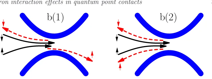
Figure 1. Illustration of the two-electron momentum-nonconserving scattering processes that give rise to a correction to the transport properties at the beginning of the first plateau. The full (black) lines represent incoming electrons, while the dashed (red) lines are the outgoing electrons. The thick (blue) lines define the edge of the
QPC. Only scattering between different spins is present to leading order inT /Tℓ
F due to the Pauli principle.
Momentum-nonconserving processes are most relevant in the low-density regime, where the Fermi wavelength is comparable to the QPC’s length, which is set by the curvature of the saddle-point potential and/or the distance to the gate electrodes[24]. Indeed, our quantitative analysis of the matrix elements for these processes (see below) shows that the effect of momentum-nonconserving scattering can be substantial, and implies that the conductance is significantly reduced at elevated temperatures, where the phase space for inelastic scattering is increased. We find that the breaking of translational invariance, and hence the backscattering rate, is most dramatic near the onset of the plateau, and then gradually decreases for larger electron density in the QPC.
We start from the assumption that the low-temperature limit of a QPC at the first quantized plateau is well described by a Fermi-liquid picture with propagating single-particle states[25]. Throughout the paper, we consider only a single transverse channel being transmitted. Without interactions and at low temperatures, T ≪ Tℓ
F
(where εℓ
F = kBTFℓ is the local Fermi energy, see (18) below), the conductance is given
by the standard Landauer-B¨uttiker[26] formula, I(0) = G
0T0(EF)V, where V is the
voltage difference across the contact andG0 = 2e2/h. In this paper, we are interested in
the properties at the plateau, i.e. when the zero-temperature transmission probability is close to one, T0 ≃ 1. At zero temperature, electrons do not experience inelastic
scattering from either phonons or other electrons. However, as temperature increases, phase space also increases for such scattering events. The effect of phonon scattering has previously been studied by Seelig and Matveev[16]. Here, we address the question of inelastic e-e scattering, which can cause electron backscattering. For example, two incoming electrons from the high-bias side can interact in the contact and scatter, so that one electron is backscattered while the other is transmitted. These processes are later denoted as b(1) and shown in figure 1. Also shown is a backscattering process for two electrons[18], which we denote as b(2). Both processes will lead to a current reduction.
barrier
Re
[image:5.612.186.365.88.237.2]ϕ
E,η(
x
)
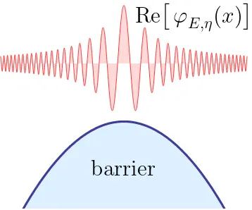
Figure 2. Illustration of the effective 1D potential of the QPC and the transmitting
wavefunctionϕE,η. The wavefunction shows an enhanced weight in the contact region,
which loosely speaking reflects the fact that electrons spend more time there. This so-called semiclassical “slowing down” is the main reason for the finite values of the backscattering processes shown in figure 1, cf. also [21], and will be discussed in section 2.3.
order in the single-particle reflection R0 = 1 − T0, be calculated using the fully
transmitting wavefunctions. To good approximation, these can be described as WKB states in an effective 1D potentialV0(x), which is a combination of the potential barrier
and the confinement barrier[25], see section 2 and figure 2. The WKB states at energy
E have the form
ϕE,η(x) =
r m
2π~p(x)exp
iη
Z x
0
dx′p(x′)/~
, (1)
where the local momentum is p(x) = p2m[E−V0(x)], m denotes the effective mass,
and η=± is the propagation direction.
For a contact with T0 ≃ 1, we may estimate the leading-order e-e interaction
correction to the current by using Fermi’s golden rule. To that end, we compute the rates for the two scattering events shown in figure 1 and add them up, with a weight factor keeping track of the respective contribution to the current. This gives the e-e interaction correction to the current in the form (e >0)
I(2) = πe
~ X
12,1′2′
|V(12,1′2′)|2η1′ +η2′ −η1 −η2
4 (2)
×n1n2(1−n1′)(1−n2′)δ(E1+E2 −E1′ −E2′),
where we use the short-hand notation 1 ={E1, η1, σ1}, withσ being the spin index, and
sums run over the quantum numbers of the scattering states,
X
1
=
Z
dE1
X
σ1=±
X
η1=±
. (3)
In (2), the occupation factorsn1 are given by Fermi-Dirac distribution functions defined
by the respective reservoirs,
n1 =fL0(R)(E1) =
1
where one should use µL for right-movers (η1 = +1) and µR for left-movers (η1 =−1),
and we have allowed for different temperatures in the two leads. Furthermore, in (2), the factor (η1′+η2′−η1−η2)/4 accounts for the change of the relative number of right-and left-moving particles from initial to final states. Equation (2) is also found from rigorous perturbation theory in the Keldysh formalism, see section 3, where the matrix elements V(12,1′2′) are specified in (44). As expected, they contain both a direct and
an exchange term, which is important for the behavior in a large spin-splitting magnetic field. The magnitude of the relevant coupling strengths is carefully estimated in section 2.3.
Based on (2), forT0 = 1, we obtain the linear conductance at low temperatures in
the form
G/G0 = 1 +G(2)/G0 = 1−Ab(πT /TFℓ)2, (5)
where a realistic estimate for a typical GaAs QPC indicates thatAb ≈1 at the beginning
of the plateau. The result (5) has also been reported in [21], where the QPC was modeled using a kinetic equation. Their prefactor Ab is proportional to an unknown
“relaxation time in the leads”, a quantity that does not appear in our theory. Instead
Ab is directly connected to the inelastic e-e interaction processes. We find that Ab
rapidly decreases when moving along the plateau, see also figure 3. The dimensionless coefficientAb includes the effects of both theb(1) and the b(2) backscattering processes.
It is also interesting to consider the interaction correction at spin-split plateaus, i.e. for large magnetic fields. Here the energy dependence of the matrix element V(12,1′2′)
becomes important for equal-spin scattering, sinceexactly at the Fermi energy the direct and exchange terms cancel for equal spins only (see section 3.2). Hence, e-e scattering corrections in the spin-polarized case are much smaller. In fact, the leading contribution turns out to be of order (T /Tℓ
F)4, and the prefactor is smaller thanAb. Physically, this
can be understood in terms of the Pauli principle. This qualitatively agrees with the experimental observation that almost no conductance suppression at the e2/h plateau
occurs.
Below we also provide results for the interaction corrections to other experimentally relevant quantities, such as shot noise, the thermopower, and the nonlinear conductance. The effect of e-e backscattering is thus most important at the beginning of the 2e2/hplateau. On the other hand, for elevated temperatures, it leads to a breakdown of
perturbation theory. Therefore, a crossover to a different type of behavior must appear. From equation (5), the temperature scale for this crossover is expected to be
T∗ ≈ T
ℓ F
π√Ab
. (6)
Contrary to the usual situation encountered in mesoscopic physics, the nontrivial question to be answered thus concerns the high-temperature limit (but still T ≪ Tℓ
F).
approaches a saturation value gs =G/G0 of order gs ≈1/2 at high temperatures. The
saturation is physically due to the fact that e-e scattering processes within the QPC region fully equilibrate outgoing electrons, which also suggests that gs is non-universal
and thus depends on the detailed form of the various e-e couplings. We mention in passing that a high-T saturation of the conductance has also been reported for long 1D wires[17, 27],
1.2. Structure of the paper
The structure of this article is as follows. In section 2, we define the model of the QPC, and provide estimates for the parameters involved. In section 3, this model is treated by lowest-order perturbation theory, and the interaction corrections to linear and nonlinear conductance, shot noise, and thermopower are computed. A simplified version of the QPC model with a local e-e interaction potential is then considered within a nonequilibrium formalism in section 4, leading to a self-consistent numerical approach. This allows us to go beyond lowest-order perturbation theory, albeit in an approximate fashion. We briefly conclude in section 5. Details of the calculations can be found in two appendices. In intermediate steps, we sometimes set~= 1.
2. Model and estimates
2.1. Model
We consider a two-dimensional electron gas (2DEG) with a single-particle potentialU(x) forming the QPC, where x= (x, y). Close to the middle of the constriction, x= (0,0), the potential is assumed to be described by a saddle-point potential[28, 29]
U(x) =U0−
1 2mω
2
xx2+
1 2mω
2
yy2, (7)
where x (y) is along (perpendicular to) the transport direction of the QPC. The QPC is thus characterized by the frequenciesωx andωy, or, equivalently, by the length scales
ℓy =
p
~/mωy and ℓx =p~/mωx. Transforming the 2D Schr¨odinger equation into 1D,
the y-direction simply gives transversal 1D subbands (modes) labeled by n= 0,1,2. . .. Therefore the effective 1D Schr¨odinger equation for moden has a potential given by
Vn(x) =~ωy(n+ 1/2) +U0−
1 2mω
2
xx2, (8)
and the well-known transmission probability through the nth mode is[28]
Tn(E) =
1
1 + exp[−2π(E−~ωy(n+ 1
2)−U0)/~ωx]
. (9)
This transmission coefficient leads to the low-temperature conductance quantization in a QPC.
with transmission close to unity,T0(EF)≃1. Therefore only the first (spin-degenerate)
mode n = 0 is included in the 1D Hamiltonian H =H0+HI. The noninteracting part
is
H0 =
X
σ
Z
dx ψσ†(x)
− ~
2
2m d2
dx2 +V0(x)
ψσ(x), (10)
and the Coulomb interaction gives
HI =
1 2
X
σσ′
Z
dxdx′ψσ†(x)ψσ†′(x
′)W(x, x′)ψ
σ′(x′)ψσ(x), (11) where ψ†
σ(x) (ψσ(x)) is the creation (annihilation) operator for the n = 0 mode. The
effective (unscreened) 1D interaction W(x, x′) can be found by integration over the
transverse eigenstates in the lowest mode, χn=0(y) = exp(−y2/2ℓ2y)/(π1/4
p
ℓy). This
gives
W(x, x′) = e
2
4πǫ0κ
√
2πℓy
M
(x−x′)2
4ℓ2
y
, (12)
whereκdenotes the relative dielectric constant,M(x) =exK
0(x), andK0is the
(zeroth-order) modified Bessel function of the second kind. This model of the interaction
W(x, x′) depends only on the difference x −x′, and therefore appears not to break
translational invariance. However, when including the scattering states, the effective interaction will break translational invariance, see the discussion in section 2.3 below.
For energies above the barrier top, the scattering states can be approximated by the WKB eigenstates (1), and we can thus expand the 1D fermion operators as
ψσ(x) =
X
η=±1
Z
dE ϕE,η(x)cE,η,σ, (13)
where the energy integral is from the top of the single-particle potential to infinity, and cE,η,σ is a scattering-state annihilation operator with anticommutation relations
{cE,η,σ, c†E′,η′,σ′}= δη,η′δσ,σ′δ(E−E
′). The noninteracting Hamiltonian then effectively
becomes
H0 =
X
1
E1c†1c1, (14)
where we again use the short-hand notation 1 = {E1, η1, σ1}, see (3). Similarly, the
interacting part reads
HI =
1 2
X
1,2,1′,2′
W1′2′,12c†1′c
†
2′c2c1, (15)
with the matrix elements
W1′2′,12 =δσ1σ
1′δσ2σ2′
Z
dx1dx2 ϕ∗E1′,η1′(x1)ϕ
∗
E2′,η2′(x2)
These matrix elements are discussed in section 2.3. For later purposes, it is also useful to introduce the corresponding matrix elements without the spin factors and taking the energies at the Fermi surface,
Wη(0)1′η2′,η1η2 =
Z
dx1dx2 ϕ∗EF,η1′(x1)ϕ
∗
EF,η2′(x2)
×W(x1, x2)ϕEF,η1(x1)ϕEF,η2(x2). (17)
Throughout the paper, we distinguish between the Fermi energy EF in the equilibrium
leads and the local Fermi energy εℓ
F in the QPC,
εℓF ≡EF −U0−
1
2~ωy =kBT
ℓ
F. (18)
The single-particle thermal smearing of the conductance plateau occurs on the energy scale εℓ
F, and therefore we are here only interested in effects at lower energies, i.e.
T ≪Tℓ F.
2.2. Hartree-Fock approximation
In order to determine the saddle-point potential (7), one should in principle solve for the potential self-consistently, including the screening by surrounding gate electrodes and mean-field interaction effects. For the electrons in the constriction, the latter amount to the Hartree-Fock approximation,
HI,HF =
X
σ
Z
dx
Z
dx′VHF,σ(x, x′)ψ†σ(x′)ψσ(x), (19)
where the self-consistent Hartree-Fock potential is
VHF,σ(x, x′) = δ(x−x′)
Z
dx′′X
σ′
W(x, x′′)nσ′(x′′)
− W(x, x′)hψσ†(x)ψσ(x′)i, (20)
with nσ(x) =hψσ†(x)ψσ(x)i. The self-consistent mean-field theory was discussed in [10],
showing that the mean-field result for theT-dependence of the conductance is markedly different from both the experimental observations and the finite-T corrections due to inelastic e-e processes studied in this paper.
To illustrate this point, let us consider the Hartree approximation. Then the change of the local density n(x) with increasing temperature follows by using a Sommerfeld expansion. Noting that the chemical potential is set by the electrodes and can be assumed constant in this temperature range, we find to lowest order in temperature
n(x) =n0(x)
"
1− π
2
24
kBT
εℓ
F +12mω2xx2
2#
, (21)
where n0(x) is the T = 0 density. First, we note that the density decreases with
potential V0(x). Expanding this result around the relevant barrier region x = 0, the
potential correction can be written as
VH(x) =δU0 + ∆
mω2
x
2 x
2+
O (x/2ℓy)4. (22)
Thereby the Hartree correction can be captured by a temperature-dependent renormalization of the barrier height U0 → U0 +δU0(T) and of the curvature ωx →
p
1−∆(T)ωx of the saddle potential in the transport direction. Explicitly, in terms of
Meijer’s G-function[30], we find
δU0 =−W
kBT
~ωx
2~
ωx
εℓ F
3/2
G32,,23 ωyǫ
ℓ F
~ω2
x 1 1 1 2 1 2 3 2 ! , (23)
with the energy scale
W = √1 18π
e2
4πǫ0κℓx
. (24)
Moreover, the dimensionless parameter ∆ follows as
∆ = 2 15
ωy
ωx
W
~ωx
kBT
~ωx
2~
ωx ǫℓ F 5 2 (25) × "
G32,,23 ωyǫ
ℓ F
~ω2
x 1 1 1 2 1 2 7 2 !
−4G32,,23 ωyǫ
ℓ F
~ω2
x 1 0 1 2 1 2 5 2 !# .
The barrier is therefore lowered, δU0 < 0, while the frequency ωx is renormalized to
smaller values, since (25) implies ∆(T) > 0. The quoted expressions are useful for
T0 ≃1, whereεℓF >~ωx/2. Inspection of (9) then shows that the net effect of the Hartree
correction is an enhancement of the transmission towards T0 = 1. As a consequence, a
conductance plateau present already at zero temperature is then essentially not affected by the Hartree contribution as long asT ≪Tℓ
F. A quantitative discussion of the Hartree
corrections to the saddle-point potential can be found in section 2.3 below.
Concerning the Fock part, a simple qualitative approximation is obtained if the pair potential is assumed to be a contact interaction, W(x, x′) = W
0δ(x−x′), see also
[10]. (This expression requires that the long-ranged tail of the e-e interaction potential is screened by nearby electrodes.) In that case, also the Fock contribution is local, and acts in precisely the same (but opposite) way as the Hartree potential, thereby partially cancelling the effects of the latter. In particular, it leads to the same temperature dependence of the corrections. We therefore conclude that the Hartree-Fock contribution leads to a very weak temperature dependence of the conductance, which even goes in opposite direction as compared to the effects of the inelastic e-e contributions. This temperature dependence of the mean-field result for the QPC conductance has been described in detail before[10, 11].
In the following, the weakT-dependence of the conductance under a single-particle picture will be neglected, and we focus on the effects of inelastic e-e scattering. Hence the interaction (11) is replaced by
When performing diagrammatic expansions, the first-order contribution inδHI vanishes
per definition, and the series starts with the second order in δHI, see sections 3 and 4.
From now on, the Hartree-Fock part is assumed to be contained in the single-particle potential V0(x).
2.3. WKB estimates for e-e matrix elements
In order for our subsequent calculations to be meaningful, it is essential to first show that the relevant e-e backscattering strengths can be sufficiently large in experimentally relevant QPC geometries. In the following, we therefore provide such estimates and demonstrate that in the beginning of the first conductance quantization plateau, these couplings are indeed significant. Let us then consider an almost perfectly transmitting QPC and calculate the matrix elements that give rise to momentum-nonconserving scattering. For a simple estimate of the relevant e-e backscattering strengths, we now employ the WKB wavefunctions, see section 1.1. For larger reflection probability the WKB approximation is not adequate and a more sophisticated approach must be used. Because of the lower electron density in the QPC region, also denoted as
semiclassical slowing down[21], interactions are strongest near the constriction, see figure 2. The single-particle eigenstates in the potentialV0(x) are given by the WKB scattering
states (1), which are a good approximation forT0(EF)≃1. The following estimates can
thus be regarded as an expansion in R0 = 1− T0, to leading order in R0 << 1. In the
WKB approximation, the matrix elements (17) for e-e scattering at the Fermi surface are given by
Wη(0)1′η2′,η1η2 = m 2π~
2Z
dxdx′ W(x, x
′)
p(x)p(x′)
× ei(η1−η1′)R0xdy p(y)/~ei(η2−η2′)Rx ′
0 dy p(y)/~. (27)
The semiclassical slowing down is reflected in the local density of states ∝ 1/p(x), which is largest inside the QPC (x= 0). Here,p(x) =p2m[EF −V0(x)] is the classical
momentum, which we express using the 1D saddle-point potential V0(x) in (8) as
p(x) = a
ℓy
~
ℓy
ωx
ωy
p
1 + (x/a)2. (28)
The Fermi energy EF enters here via the length scale a,
a ℓy
= ωy
ωx
s
2(EF −U0−~ωy/2)
~ωy . (29)
This scale can also be related to the transmissionT0(EF) by using (9), and hence to the
position along the first conductance plateau. Inverting (9), we find
a ℓy
2
= 1
π ωy
ωx
ln
T0
1− T0
, (30)
valid for 0.5≤ T0 <1. Next, consider the integral in the phase factor of (27),
γ(ξ)≡ 1
~ Z x
0
εℓ
F TFℓ a/ℓy T0(EF) fb(1) Wb(1) Ab(1) 2
9~ωy 2.3 K 2.0 0.985 0.64 720 eV
−1 1.1 1
2~ωy 5.2 K 3.0 1.0 3.0×10
−2 34 eV−1 1.0×10⁻² 7
9~ωy 8.1 K 3.7 1.0 1.0×10
[image:12.612.69.522.231.429.2]−3 1.1 eV−1 1.5×10⁻⁵
Table 1. Estimates for the interaction matrix elementsWb(1) andAb(1), see (35), at
three different positions on the first conductance plateau, i.e. versus the local Fermi
energyεℓ
F. Parameters are: ~ωx= 0.3 meV,~ωy= 0.9 meV,κ= 10 andm= 0.067me.
See also figure 3.
= 1 2π ln
T0
1− T0
h
ξpξ2+ 1 + lnξ+pξ2+ 1i,
where ξ=x/a. This expresses (27) in a form suitable for numerical integration,
Wη(0)1′η2′,η1η2 = 1 (2π~ωx)2
e2
4πǫ0κℓy
fη1′,η2′,η1,η2 (32)
where
fη1′,η2′,η1,η2 =
1 √ 2π Z ∞ −∞ dξ Z ∞ −∞
dξ′p 1 ξ2+ 1
1
p
ξ′2+ 1
×M
"
(ξ−ξ′)2
4 a ℓy 2# (33)
×cos[(η1 −η1′)γ(ξ) + (η2−η2′)γ(ξ′)]
with M(x) defined after (12). The matrix elements for the b(1,2) scattering processes in figure 1 correspond to
Wb(1) =W++(0),+−, Wb(2) =W++(0),−−, (34)
while e-e forward-scattering processes are described byWb(0) =W++(0),++. The couplings
Wb(i) enter the current through the dimensionless parameters
Ab(i) =
16π2
3 (kBT
ℓ
FWb(i))2 =
1 12π2
"
1
~ωy
e2
4πǫ0κℓy
a ℓy
2
fb(i)
#2
. (35)
We now use typical experimental parameters for a GaAs QPC:[31] ~ωx = 0.3 meV, ~ωy = 0.9 meV, κ = 10 and m = 0.067me. We have numerically integrated fb(1) at
three different values of the local Fermi levelεℓ
F, see table 1. Clearly, Wb(1) becomes two
orders of magnitude smaller from the beginning of the conductance plateau to the end, while Ab(1) differs even by five orders of magnitude, see figure 3.
Let us then briefly discuss the magnitude of the Hartree corrections mentioned in section 2.2. Given the QPC parameters in figure 3, we obtain the energy scale
W ≈ 0.31 meV from (24). It is then possible to compare the Hartree conductance correction to the respective inelastic correction (5). For concreteness, we takeT = 0.7K, corresponding to T∗ at the beginning of the plateau in figure 3. From (23), at the
positions of the arrows in figure 3, we find δU0 ≈ −0.24 meV, −0.08 meV, and
0 0.2 0.4 0.6 0.8
2
e
2h
A
b(1)=1
.
1
A
b(1)=0
.
010
A
b(1)=1
.
5
×
10
−5 [image:13.612.171.440.84.239.2]Considered energies
ε
ℓF[meV]
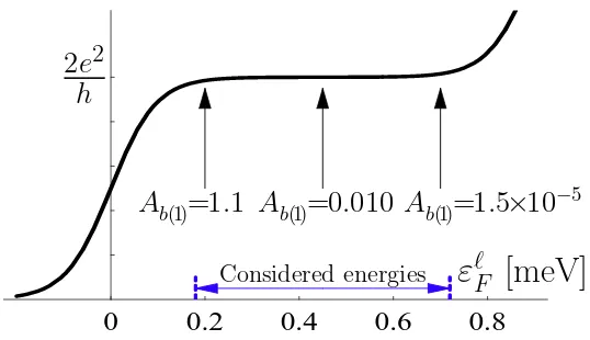
Figure 3. The interaction matrix elements for backscattering of a single electron
at various positions on the first quantized conductance plateau. The solid curve
shows theT = 0 conductance vs εℓ
F for a saddle-point potential with~ωx = 0.3meV
and ~ωy = 0.9meV. The decrease of the conductance in (45) is then orders of
magnitude stronger in the beginning of the plateau. The backscattering of one
electron (Ab(1)) is significantly stronger than that of two (Ab(2)). NeglectingAb(2), the
conductance corrections for the three values ofAb(1) are: G(2)/G0 =−2.1K−2×T2,
G(2)/G
0=−3.6×10⁻³K−2×T2 andG(2)/G0=−2.2×10−6K−2×T2, respectively.
ForT =T∗, we haveG(2) =G
0, and perturbation theory fails. This corresponds to
T∗= 0.7K,T∗= 17K, andT∗= 670K for the three stated values ofA
b(1). Therefore,
it is desirable to go beyond a perturbative treatment. The quoted Ab(1) values are
found numerically by integration of (33).
∆≈ 0.77,0.13, and 0.05, respectively. The Hartree corrections to the conductance are then captured by (9), and imply an increase of the conductance. Since for all three cases in figure 3, the transmission at zero temperature is T0 ≥0.985, the Hartree correction
can at most enhance the conductance by a factor≈1.015, which is a much smaller effect than the inelastic corrections discussed in this paper. Note that including the Fock term reduces the found Hartree contribution even further.
Finally, screening by higher (closed) subbands and by nearby gate electrodes also leads to an interaction with broken translational invariance, where the effective interaction range is set by a combination of the pinch-off distance for closed subbands and the screening length of the electrodes. This would have two consequences, namely (i) an overall decrease of the e-e interaction strength, and thus of the Ab(i), and (ii) an
additional source for broken translational invariance, which enhances theAb(i). The net
result of including screening by the adjacent gates and 2DEG regions is therefore not straightforward, and a detailed electrostatic calculation is needed to gain a reliable understanding. Since semiclassical slowing down already results in very significant backscattering amplitudes, we focus on that in the present paper.
3. Perturbation theory
treat the interaction Hamiltonian δHI by perturbation theory, yielding the current as
I =I(0)+I(2)+· · ·. We here employ the Keldysh formulation to compute the correction
I(2) due to inelastic e-e scattering to second order in the interaction, and start with the
definition of the current
I =ieX
11′
h1′|Jˆ(x)|1iG<(11′, tt), (36)
where G<(11′, tt′) = ihc†
1′(t
′)c
1(t)i is the nonequilibrium lesser Green’s function (GF),
and ˆJ(x) = ~
2mi( − →∂
x −←∂−x). For T0 ≃ 1, we can use the WKB states in (1) to calculate
the current matrix element,
h1′|Jˆ(x)|1i=δσ1σ1′ 1 4π~
η1p1(x) +η1′p1′(x)
p
p1(x)p1′(x)
×exp
i
~ Z x
0
dy[η1p1(y)−η1′p1′(y)]
. (37)
Here, we neglect terms proportional to ∂xp(x) to be consistent with the WKB
approximation. In order to also allow for different temperatures in the two leads, we employ the nonequilibrium formalism in a slightly different way than usual[32, 33], namely we include the different chemical potentials and temperatures in the initial density matrix ρ0(H). (The left/right reservoirs inject electrons distributed by Fermi
functions (4).) The interaction Hamiltonian δHI is treated as the perturbation that
connects the two reservoirs. To evaluate the current, we thus write
I = Tr[ρ(H0) ˆJ(x, t)], (38)
where ˆJ(x, t) is in the Heisenberg picture, ˆJ(x, t) ≡ eiHt/~ˆ
J(x)e−iHt/~
. Here H =
H0+δHI, and
ρ(H0) =Z−1e−(H0,L−µLNL)/kBTL−(H0,R−µRNR)/kBTR, (39)
where NL/R and H0,L/R are the number operators and noninteracting Hamiltonians,
respectively, for electrons coming from the left/right lead. The noninteracting (retarded, advanced, lesser, and greater) GFs then follow in the form[32]
G0r/a(1, ω) =
1
ω−E1±i0+
(40)
G0<(1, ω) = 2πin1δ(ω−E1),
G0>(1, ω) = −2πi[1−n1]δ(ω−E1),
wheren1 is given in (4). The GF’s are diagonal in spin space and identical for both spin
directions.
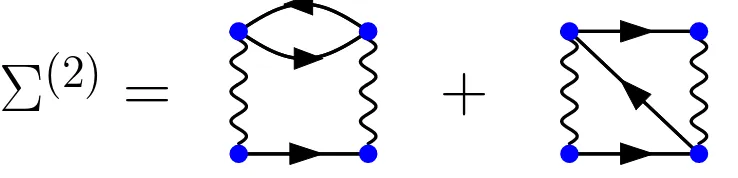
We now use a diagrammatic expansion of the interaction operator in terms of contour-ordered GFs[32]. Since the first-order diagrams vanish per definition, the leading diagrams are given by the second-order self-energy diagrams shown in figure 4. The second-order correction to the lesser GF can be found by using standard Langreth rules[32] cf. (73). After some algebra, employing (40), we obtain
I(2) =ieX
11′
Z dω
2π~
h1′|Jˆ(x)|1i
E1−E1′ −i0+
Σ
(2)
=
+
Figure 4. The second-order diagram included in (43). The first-order and all other second-order diagrams belong to the self-consistent Hartree-Fock sector and are contained in the saddle-point potential, see section 2.2. To avoid double-counting, they should therefore not be taken into account here.
−Σ(2)r(11′, ω)G0<(1′, ω) +G0<(1, ω)Σ(2)a(11′, ω) . (41) One checks that this expression conserves current by differentiating with respect to
x, and therefore we can set x = 0. Now there are two contributions to the current, corresponding to the real and imaginary parts of [E1−E1′ −i0+]−1, where symmetry arguments show that the real part must vanish. For the imaginary part, we have a
δ-function enforcing E1 = E1′, which then, see (37), implies η1 = η1′. This leaves us with
I(2) =−ie 2~
X
1
η1
(1−n1)Σ(2)<(11, E1) +n1Σ(2)>(11, E1)
,
where we use Σ(2)r −Σ(2)a = Σ(2)>−Σ(2)<. The lesser self-energy has two parts, the
direct and the exchange contribution, corresponding to the two terms in figure 4. In the time domain, this gives
Σ(2)<(11, tt′) =−X
234
G0<(2, tt′)G0>(3, tt′)G0<(4, tt′)(W13,24−W31,24)W24,13.(42)
The expression for Σ(2)> follows by interchange of lesser and greater GFs in (42). After
a number of manipulations, we reduce this to
I(2) = − eπ
~ X
1,2,1′,2′
|W12,1′2′ −W21,1′2′|2 1
8(η1+η2 −η1′ −η2′)
×[n1′n2′(1−n1)(1−n2)−(1−n1′)(1−n2′)n1n2]
×δ(E1+E2−E1′−E2′). (43)
In fact, this result recovers the Fermi golden rule expression (2), as may be seen by combining the two terms in (43). We can now read off the matrix element entering (2),
3.1. Conductance at low temperatures and voltages
The perturbative interaction correction (43) to lowest order in temperature T ≪ Tℓ F
and voltageeV ≪εℓ
F is determined only by the interaction matrix elements (17) taken
at the Fermi surface. Some algebra then gives
I(V, T)
G0V
=T0(EF)− Ab(1)+Ab(2)
πT Tℓ F
2
(45)
−
A
b(1)
4 +Ab(2)
eV εℓ
F
2
+O Wb3(i),
with the dimensionless coefficients Ab(1,2), see (35), corresponding to b(1) and b(2)
processes for electrons at the Fermi surface. We stress again that (45) holds only to lowest order in R0 = 1− T0, i.e. close to unity transmission at zero temperature. As
described in section 1.1, the processb(2) corresponds to the simultaneous backscattering of two electrons, which has been discussed on a perturbative level in [18]. The process
b(1), where a single electron is backscattered, has not been studied before. It is here important to note that for both processes, low-energy scattering is only possible between opposite spins: When the energy arguments in the matrix element (44) are taken at the Fermi energy, the direct and exchange terms cancel each other for equal spins. The parameter Ab(1) is expected to dominate over Ab(2), and has been estimated in section
2.3 for a typical GaAs QPC. We found that Ab(1) changes from ≈1 to≈10−5 from the
beginning of the first quantized conductance plateau to the end, see figure 3 and table 1. From (45), we observe that interaction processes that do not change the number of left- and right-movers give no contribution to the current correction I(2). The
same conclusion is reached for finite-length quantum wires using a Boltzmann equation approach[34, 35]. In particular, forward-scattering processes do not contribute to I(2),
even though total momentum is not necessarily conserved in these processes either. Here, the important point is only whether the number of left- and right-moving electrons is conserved or not. However, at higher orders, important at elevated temperatures, all e-e interaction processes can come into play, see also Appendix A of [35].
3.2. Spin-polarized case
Next we consider the effect of interactions for a completely spin-polarized QPC in a large magnetic field, i.e. on the e2/h plateau. For the spin-degenerate case, we found above
that to leading order in T /Tℓ
F, only opposite spins interact due to the Pauli principle.
As a consequence, the conductance correction is further suppressed for a single spin species, as we shall show now. In the spin-polarized case, we must take into account the energy dependence of the interaction matrix elements W12,1′2′, which leads to a stronger power-law suppression in temperature. The current correction to second order in the interaction for a single spin species follows from (43), and in linear response, we find
I(2) = − eV
kBT
2eπ
~ Z
dE1dE2dE1′dE2′ |Vb(1)k|2+|Vb(2)k|2
where the ni are taken for µR = µL = EF. The same-spin interaction matrix elements
are
Vb(1,2)k =WE1+↑,E2+↑,E1′±↑,E2′−↑−WE1↔E2,
i.e. a direct term minus an exchange term, whereE1 and E2 are interchanged. Here, the
index E1′+↑ [E1′− ↑] refers to the b(1) [b(2)] process. To lowest order in temperature, the leading term is found by expanding the Vb(1,2)k around the Fermi energy, since
Vb(1,2)k = 0 when all energies are equal to EF. The low-temperature interaction
correction to the spin-polarized linear conductance G(0)=e2/h is obtained as
G(2)=−2e
2
h Bb(1)
πT
Tℓ F
4
, (47)
where the dimensionless parameter
Bb(1) =
32π2
15 (kBT
ℓ F)4
(∂E1 −∂E2)Wb(1)↑|EF 2
(48)
with Wb(1)↑ = WE1+↑,E2+↑,E1′+↑,E2′−↑ is estimated in Appendix A. There, we find
Bb(1) ≈0.1 at the beginning of the quantized plateau (forT0(EF) = 0.985, corresponding
to the first arrow in figure 3). For theb(2) process, the resulting power-law suppression is even of higher order, since
(∂E1 −∂E2)Wb(2)↑|EF
2 = 0, (49)
where Wb(2)↑ =WE1+↑,E2+↑,E1′−↑,E2′−↑. To get (49), we use W12,1′2′ = W21,2′1′, which in turn follows fromW(x, x′) =W(x′, x). In conclusion, an extra factor (T /Tℓ
F)2suppresses
the low-temperature correction at the spin-polarizede2/hplateau (i.e. the large-B case)
as compared to the spin-degenerate 2e2/h plateau (i.e. the B = 0 case).
3.3. Noise
Next we calculate consequences for another observable, namely nonequilibrium quantum noise. The zero-frequency shot noise follows from the (symmetrized) two-point correlation function of the current operator. Perturbation theory yields for the backscattering noise power in zero magnetic field
SB(V, T) = 2e
h
2Ibs(2)(V, T) coth(eV /kBT)
+Ibs(1)(V, T) coth(eV /2kBT)
i
, (50)
where Ibs(1,2) are the current corrections due to Wb(1,2) quoted in (45) (defined positive
for V > 0). This is nothing but the famous Schottky shot noise relation, encoding the charge of the backscattered particles. Equation (50) predicts an additional factor of two for the b(2) contribution, because two electrons are backscattered in that event[18].
The direct perturbative calculation of the noise to second order in δHI then yields
the full noise power of the transmitted current in the compact form
where Ibs =Ibs(1)+Ibs(2). This perturbative result has also been obtained in a different
context before[36]. In the limit V → 0, one recovers the expected thermal Johnson-Nyquist noise 4kBT[G0+G(2)(T)] from (51), with the interaction correctionG(2)specified
in (5). Note that the last term in (51) ensures that the correct thermal noise formula is obtained.
Recent noise measurements on the first quantized plateau were compared to the corresponding single-particle picture[7], and a reduced noise power was observed at the conductance anomaly. Let us now connect (51) to this discussion. For that comparison, according to [7], one subtracts the thermal noise and defines the excess noise as
SI =ST −4G(V, T)kBT. (52)
For a noninteracting system, this quantity is given by
SISP = 2G0Re[eV coth(eV /2kBT)−2kBT] (53)
to lowest order in the reflection coefficient Re, see reference [7]. In order to compare our approach to (53), we interpret Ibs/G0V in a single-particle picture as an effective
reflection probability Re. Of course, this reflection is now mainly caused by interaction processes, and Re is generally larger than the true noninteracting value R0. Therefore,
the difference between the true excess noise and its single-particle value is, in this framework, given by
SI−SISP
2G0eV(T /TFℓ)2
=−2Ab(1)
eV kBT
+Ab(2)h(eV /kBT), (54)
where
h(x) =−8x+ (π2+x2) tanh(x/2). (55)
From this expression, one observes that for eV < 6.507 kBT, regardless of Ab(1,2),
the measured noise should always be smaller than predicted by a single-particle analysis. This situation precisely corresponds to the parameter range of relevance for the experimental work of reference [7], where eV . 5kBT. Our results for the noise
are therefore consistent with the conclusions reached in reference [7]. Unfortunately, however, we cannot compare to the shot noise line profiles reported in Ref. 7, because our results are only valid to lowest order in R0, and such line profiles would require a
calculation as a function of R0.
3.4. Thermopower
Another experimental observable probing the enhanced phase space for e-e scattering at T 6= 0 is the thermopower S(T)[5, 37], for which perturbation theory for the spin-degenerate case predicts
S(T) = kB
e
2π4
5 Ab(1)+Ab(2)
T
Tℓ F
3
Since the noninteracting thermopower is exponentially small [∝ exp(−Tℓ
F/T)] at
the conductance plateau, the interaction correction completely determines the low-temperature thermopower[34]. The enhanced thermopower (as compared to the noninteracting one) is in qualitative agreement with experiments at the anomalous plateau[5, 6].
4. Self-consistent nonperturbative scheme
As discussed in section 1.1, the intermediate temperature regime
T∗ .T ≪TFℓ (57)
needs to be understood beyond perturbation theory, see the caption of figure 3 for typical values of T∗. Let us first discuss, on a qualitative level, what happens in limiting cases,
where the QPC transport problem can be solved without invoking approximations. For instance, when Ab(0,1) = 0 but Ab(2) 6= 0, one can establish correspondence to
the problem of a single impurity in a Luttinger liquid with interaction parameter
K = 2, which in turn is solvable[38] and leads to the high-temperature saturation value gs =G(T ≫T∗)/G0 = 0 of the linear conductance. Physically, this is quite clear:
With strongb(2) interactions, all particles are backscattered for increasing phase space, and the conductance approaches zero. Similarly, when Ab(1,2) = 0 but Ab(0) 6= 0, i.e.
when only forward scattering is present, the conductance is not affected at all, gs =T0
for T0 ≃ 1. (However, for T0 < 1, forward scattering can increase the conductance,
since such processes give an additive contribution to the usual elastic transmission.) Unfortunately, the most interesting special case, Ab(0,2) = 0 but Ab(1) 6= 0, seems not
described by an exactly solvable model. With only strong b(1) interactions present, all particles scatter in the QPC, but half of them are still transmitted. This suggests a reduction of the conductance by a factor of two, gs = 1/2.
In order to make quantitative progress, we now consider a simplified model. It is given by the noninteracting part (10) with V0(x) = 0. Therefore, we now have the
situation EF = εℓF ≡ εF = kBTF. Moreover, we take the interacting part (11) with a
local pair potential, see also [21],
W(x, x′) =fW δ(x)δ(x′). (58) The local nature of the pair potential implies that all e-e interaction processes have the same amplitude, i.e. the amplitudes for backscattering of one and two electrons and the forward-scattering amplitudes are all equal, Ab = Ab(0) = Ab(1) = Ab(2).
This is an artefact of the oversimplified local interaction (58). Nevertheless, a study of this problem is useful as it allows for an explicit calculation of the crossover from the T2 corrections to the high-temperature conductance saturation. The model cannot
most important effect of a large B-field, which consists of quenching the backscattering amplitudes, cf. section 3.2, is missed. We then only consider B = 0 for the remainder of this section. For convenience, we express the interaction strength in terms of a dimensionless parameter,
λ=mfW /2~2π3/2. (59)
Writing λ in terms ofAb, we find[39]λ=
p
3Ab/π. On the first part of the plateau, we
found Ab(1) ≈1, see section 2.3, with T∗/TF .0.3. This allows for a meaningful study
of the temperature range (57) with λ <1.
In order to treat the local interaction (58), we start from the Dyson equation for the full Keldysh single-particle GF Gσ(x, x′;ω) for spin σ, which is a 2×2 matrix in
Keldysh space. Note that the interaction (58) does not flip the spin, and therefore the Dyson equation is
Gσ(x, x′;ω) =G0;σ(x, x′;ω) +G0;σ(x,0;ω)Σσ(ω)Gσ(0, x′;ω), (60)
where the self-energy acts only atx=x′ = 0.Moreover, both spins enter symmetrically,
G↑ = G↓, and we can suppress the spin index. In Appendix B, we show that for the
interaction (58) and a parabolic dispersion, εk =k2/2m, the current can be expressed
in terms of the local spectral function (at x=x′ = 0) only,
I = e
h
X
σ
Z ∞
0
dωfR0(ω)−fL0(ω)Aσ(ω)
A0(ω)
, (61)
where the Fermi functions are defined in (4), and the local spectral function is
A(ω) = i[Gr(ω)− Ga(ω)] =−2 ImGr(ω) (62)
with G(ω)≡ G(0,0;ω). The noninteracting spectral function is
A0(ω) = 2πd(ω) = (2m/ω)1/2θ(ω), (63)
where d(ω) is the density of states, and θ the Heaviside step function. Note that the real part of the noninteracting retarded GFGr
0(ω) is nonzero atω <0 for this dispersion
relation,
G0r(ω) =
Z dk
2π
1
ω−k2/2m+i0+
= −πd(ω) (θ(−ω) +iθ(ω)). (64)
In effect, the nonequilibrium current through the interacting QPC, (61), is fully expressed in terms of the local retarded GF only.
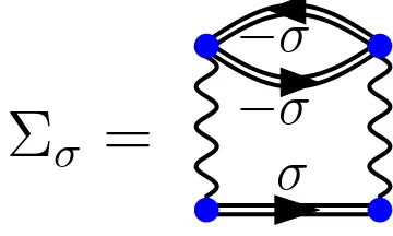
Σ
σ
=
σ
−
σ
[image:21.612.182.362.92.200.2]−
σ
Figure 5. The self-consistent second-order diagram for the spin directionσincluded in our SCBA scheme for the treatment of interactions. Double lines define full (self-consistent) GFs, as opposed to thin lines describing noninteracting GFs, see figure 4. Note that the exchange term exactly cancels the direct contribution for same spins, and therefore the second diagram in figure 4 does not appear here.
perturbative calculations of section 3, the noninteracting GF enters instead, cf. figure 4. In particular, the retarded component of the self-energy is
Σrσ(ω) =Wf2
Z ∞
0
dteiωtG−<σ(−t)Gσ>(t)G−>σ(t)− G−>σ(−t)Gσ<(t)G−<σ(t),(65) where G≶
σ denotes the local lesser/greater GF of the interacting system. The SCBA
approach is similar in spirit to using a quantum Boltzmann equation approach with a self-consistent two-body collision integral, see Sec. 6.7.2 in [41] for a detailed discussion.
4.1. Linear transport
We first discuss the linear conductance, where the spectral function in (61) can be calculated in equilibrium. Thus, the lesser/greater GFs can be written in terms of the spectral function,
G<(ω) = iA(ω)f0(ω), G>(ω) = iA(ω)(f0(ω)−1), (66) where f0(ω) = 1/[e(ω−εF)/kBT + 1]. Note that when evaluating G≶(t) as needed in (65),
G≶(t) =
Z ∞
−∞
dω
2πe
−iωtG≶(ω), (67)
negative frequencies have to be kept, cf. (64). Consequently, the self-energy and the interacting spectral function A(ω) are generally nonzero at ω < 0 due to the presence of interactions. However, the current only depends on the spectral functions at ω >0, see (61).
To solve the self-consistency problem, we have employed an iterative procedure. Starting with the initial guess of the noninteracting GF, G(ω) = G0(ω), see (64) and
(66), we compute Σr(ω) from (65), which in turn defines a new retarded GF and a new
guess for A(ω) from the Dyson equation (60). In the linear response regime, only the retarded part of (60) is needed,
With the solution to (68), we then compute a new estimate for Σr(ω), and iterate the
procedure until convergence has been reached. In the numerical implementation, it is essential to employ fast Fourier transformation routines to switch between frequency and time space, cf. (67). This permits the fast evaluation of the self-energy (65) in time space. For coupling strengths λ < 0.8, this numerical scheme converges to a unique solution for the spectral functions A(ω), and can be implemented in an efficient manner. For larger λ, however, several solutions may appear, and the approximation appears to be ambiguous. We therefore do not show results in this regime. Given the converged spectral function, we can compute the linear conductance G from (61) by replacing f0
R−fL0 → eV[−∂ωf0(ω)]. Thereby, G is numerically obtained as a function
of the dimensionless parameters λ and T /TF.
Let us first briefly discuss the lowest-order result for the retarded self-energy (65) at T = 0. The result is obtained by first inserting (66) with A(ω) → A0(ω), see (63),
into (67). We find
G0<(t) =
im
2π2t
1/2
γ(1/2, iεFt), (69)
with G0>(t) following by overall sign change and γ → Γ, with the incomplete gamma
functions γ(α, x) and Γ(α, x)[30]. For the chosen dispersion relation, we thereby get an UV-singular behavior in the self-energy Σr(t) from (65), which manifests itself in the
t→0 behavior
Σr(t→0)≃ −fW2θ(t)m
√
2mεF
π2t
1 +O(t1/2). (70)
This divergence is also present at finite temperature, but affects only the real part of the self-energy. The perturbative results in section 3 are thus insensitive to it. However, when performing a nonperturbative calculation, a regularization of this UV divergence becomes necessary, and we chose a bandwidth cutoff of the order ωc ≈3εF around the
Fermi level. It is numerically convenient to employ a smooth cutoff function (e.g. a 1/cosh2 filter), but the precise choice for the cutoff function does not appear to affect our results below.
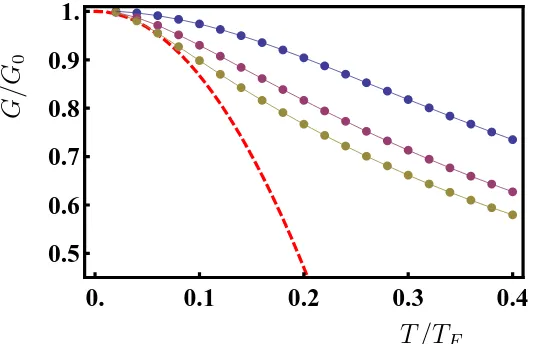
The numerical results for the linear conductance are shown in figure 6. First of all, we accurately recover the perturbation theory results at lowT. At higher temperatures, a trend towards a conductance saturation could be conjectured from the numerical data. On a qualitative level, this saturation value could be expected from the following simple consideration. In the beginning of section 4, we discussed that including only one of the backscattering processes of zero, one, or two electrons could lead to a high-temperature saturation value ofgs = 2,1,or 0, respectively. Since the point-like interaction gives the
same amplitude to all three processes, it is tempting to simply take an average of the processes and conjecture a saturation value ofe2/hfor this model.
0.
0.1
0.2
0.3
0.4
0.5
0.6
0.7
0.8
0.9
1.
T /T
FG
/G
[image:23.612.144.411.87.259.2]0
Figure 6. Temperature dependence of the linear conductanceGaccording to the
self-consistent numerical approach described in section 4.1 forλ= 0.3,0.6,and 0.8 (from
top to bottom curve). The dashed curve gives the perturbative result forλ= 0.8, dots
refer to the numerical data, and solid curves are guides to the eye only.
functions, slightly generalized to allow for different high-T saturation values. The activated behavior is
G(T)
G0
= 1−(1−gs,λ)e−T ∗
λ/T, (71)
wheregs,λcharacterizes the high-T saturation value, andTλ∗corresponds to the crossover
temperature scale (6). The Kondo-like equation used for comparison with experimental data[4] is a scaled and shifted version of the universal scaling curve known from the Kondo problem. (However, this type of modification is not justified within the Kondo model, where G→0 at high T.) We can get reasonable fits to both of these functions, see also [41].
As a final remark on the numerical solution of the self-consistent approach in the linear regime, we mention that the thermopower (data not shown) exhibits a crossover from the S ∝T3 law at low T, see (56), to a linear-in-T behavior at elevated
temperatures.
4.2. Nonlinear transport
The iterative solution of the self-consistency problem is also possible out of equilibrium, and thereby allows to compute the nonequilibrium current (61). The iteration now has to supplement (65) for Σr by the corresponding equations for the greater/lesser
components of the self-energy,
Σ≶σ(ω) = fW2
Z ∞
−∞
dteiωtG−≷σ(−t)Gσ≶(t)G−≶σ(t). (72)
0.
0.25
0.5
0.75
1.
1.25
1.5
0.5
0.6
0.7
0.8
0.9
1.
eV /ε
FG
/G
[image:24.612.145.410.87.264.2]0
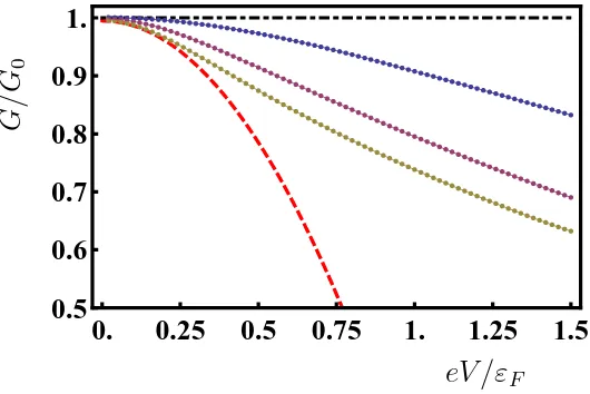
Figure 7. Self-consistent numerical results for the voltage-dependence of the
nonlinear conductance G =I/V for λ= 0.3,0.6,0.8 atT = 0.02TF (dotted curves,
from top to bottom). For λ = 0.8, also the comparison to the perturbative result
(dashed curve) is shown. For the noninteracting case,G≃G0 foreV <2εF (shown
as black dash-dotted curve).
relation
G≶(ω) =G0≶(ω) +G0r(ω)Σr(ω)G≶(ω) (73) +G0r(ω)Σ≶(ω)Ga(ω) +G0≶(ω)Σa(ω)Ga(ω),
where the advanced components (Ga, Σa) simply follow from the respective retarded
ones by complex conjugation, since they are defined locally at x = x′ = 0. For the
iterative procedure, the initial values are now given by the lesser/greater noninteracting GFs
G0<(ω) =iπd(ω)θ(ω)[fR0(ω) +fL0(ω)], (74) G>
0 (ω) =iπd(ω)θ(ω)[fR0(ω) +fL0(ω)−2].
The iterative scheme can then be set up in a very similar manner, and yields a self-consistent solution for the local spectral functionA(ω), which in turn allows to compute the current from (61). As a check, in the linear response regime of small bias voltage, we have reproduced the results of section 4.1.
Numerical results for the nonlinear conductance G(V, T) = I/V at a very low temperature are shown in figure 7. A clear decrease of the conductance with increasing
V is observed, with a tendency towards saturation of the nonlinear conductance for large voltages.
5. Discussion and conclusion
conductance (including their magnetic field dependencies), thermopower, and shot noise at the 0.7 anomaly. The gate-voltage dependence can also be qualitatively explained within the present scheme. The lack of translational invariance caused by a saddle-point potential is significant for realistic parameters often used to describe experimental realizations of QPCs. It is, however, also noteworthy that for longer quantum wires, where a saddle-point potential is not applicable anymore, similar backscattering effects can be caused by the lack of translational invariance at the ends of the quasi-1D wires. The self-consistent GF formalism for a simple point-like interaction model indicates that the conductance may approach a constant but non-universal value of order≈e2/h
at high temperatures. The precise saturation value is expected to depend on the detailed e-e backscattering parameters, and hence on the detailed geometry of the QPC. The saturation should appear in the temperature dependence of the linear conductance. Our numerical data are also consistent with a saturation effect in the voltage dependence of the nonlinear conductance, but this issue requires further study. Physically, the saturation is caused by a relaxation of the incoming electron distribution functions due to the interactions within the QPC region. It should therefore be possible to develop a Boltzmann-type kinetic equation approach to describe (nonequilibrium) inelastic scattering in a QPC, see also [21] for attempts in this direction. However, such a development is not an entirely straightforward procedure and is outside the scope of this article.
It is also instructive to discuss the point-like interaction model (58) in terms of an Anderson impurity model, see [41] for details. By spatial discretization this Hamiltonian maps onto a 1D tight-binding chain with hopping matrix elementstand on-site interactionU acting at one site (x= 0) only. In order to have perfect transmission atT = 0 for the Anderson model also, the one-particle on-site energy must be canceled out so that the local energy is ǫ0 = εF −ReΣr(εF). We thus arrive at an
Anderson-type impurity model similar to the one used in [13] to describe interactions in a QPC in the Kondo regime. However, we consider a rather different parameter regime where
U is of the same order as the hybridization Γ and can be parametrically larger than the bandwidth D ∼ |t|. Employing (6) with εℓ
F ≈ D, the interesting temperature
range (57) translates to D2/U < k
BT ≪ D. While the Kondo model requires the
formation of a local moment, this is not the case for the present approach. It would be interesting to explore this new parameter regime of the Anderson model by other non-perturbative schemes developed for the Anderson model. We believe that our theory offers a complementary approach to the 0.7 anomaly, which is not based on the assumption of a (quasi-)bound state in the QPC. In real samples, however, extrinsic effects (e.g. disorder) may be responsible for the presence of a bound state, and both mechanisms may then be relevant in parallel.
In the latter case, interaction effects due to semiclassical slowing are in principle also present on the higher conductance plateaus. However, in this case the other completely open channels screen the effective interaction, resulting in a presumably much smaller effect as compared to the first plateau. While we have repeatedly mentioned the experimental observations related to the 0.7 anomaly as the main motivation for our work, it is also clear that a realistic and quantitative description of experiments needs to consider a more refined modelling. This is especially important for the proper description of magnetic field effects away from the perturbative high magnetic field limit described in section 3.2. Moreover, on the theoretical side, it would be highly desirable to go beyond our perturbative calculation in a more realistic model. For instance, the gate-voltage dependence of the conductance at elevated temperatures – giving rise to the shoulder-like feature associated with the 0.7 anomaly – is not accessible to our theory at the moment, neither in the perturbative regime nor for the point-like interaction model in section 4, where the gate-voltage dependence is difficult to incorporate. In any case, we hope that the model calculations discussed here can give new insights into the physics behind the observed anomalies in quantum point contacts.
Acknowledgments
We thank P. Brouwer, M. B¨uttiker, W. H¨ausler, J. Paaske, and E. Sukhorukov for discussions. A.M.L. appreciates the support by the Swiss National Science Foundation. We acknowledge support by the SFB TR 12 of the DFG and by the ESF network INSTANS.
Appendix A. Calculation of Bb(1) in the WKB approximation
Here we estimate (48) for the prefactorBb(1)of the T4 interaction correction to the
spin-polarized conductance plateau e2/h, see (47). The large B-field scattering amplitude
involves a derivative of the WKB states with respect to energy,
∂EϕE,η(x) =ϕE,η(x)
−12p2m(x) + i
~η Z x
0
dy m p(y)
.
When inserting this into (48), we obtain
(∂E1 −∂E2)Wb(1)↑|EF =
m
2π~
2 e2
4πǫ0
√
2πκℓy
Z ∞
−∞
dx
Z ∞
−∞
dx′ 1 p(x)p(x′)
×M
(x−x′)2
4ℓ2
y
exp −2i
~ Z x′
0
dy p(y)
!
× 2p2m(x′) −2pm2(x)+ im
~ Z x′
x
dy p(y)
!
. (A.1)
Using the same parametrization as in section 2, this becomes
(∂E1 −∂E2)Wb(1)↑|EF =
1 (2π~ωx)2
e2
4πǫ0κℓy
1
where
gb(1)=
1 √ 2π Z ∞ −∞ dξ Z ∞ −∞
dξ′p 1
ξ2+ 1
1
p
ξ′2+ 1M
"
(ξ−ξ′)2
4 a ℓy 2# × " 1 2 ℓy a 2 ωy ωx 2 1 1 +ξ′2 −
1 1 +ξ2
cos[2γ(ξ′)]
+ωy
ωx
sinh−1(ξ′)−sinh−1(ξ)sin[2γ(ξ′)]
.
The value of Bb(1) is therefore given by
Bb(1) =
1 120π2
a ℓy 8 ωx ωy 4 e2
4πǫ0κℓy
1
~ωy gb(1) 2
.
Numerical integration for the same parameters as in section 2.3 (~ωx = 0.3 meV, ~ωy = 0.9 meV, κ= 10, m = 0.067me, and a/ℓy = 2) then yields Bb(1) ≈0.1.
Appendix B. Current for local interaction model
The purpose of this appendix is to derive (61) for the point-like interaction (58). The derivation is a rewriting of the expectation value of the current operator, see (38) and (39),
I(x, t) = ~ 2mi
X
σ
ψ†(xt)(∂xψ(xt))−(∂xψ†(xt))ψ(xt)
,
where x is arbitrary, ψ†(xt) is the creation operator in the Heisenberg picture, and the
spin index is suppressed. In terms of the lesser GF G<(xx′, tt′) = ihψ†(x′t′)ψ(xt)i, the
average value is rewritten as
hIi= ~ 2m X σ Z ∞ −∞ dω
2π xlim′→x[∂x
′ −∂x]Gσ<(xx′, ω). (B.1) Since the current is independent of x, we may take x = 0 to evaluate it. To find
∂xG<(xx′, ω) and ∂x′G<(xx′, ω), the Dyson equation is used. The point-like interaction (58) allows to simplify the Dyson equation from an integral equation to an algebraic one. Using the Langreth rules[32], we obtain for the lesser GF
G<(xx′, ω) =G0<(xx′, ω) +G0r(x0, ω)Σr(00, ω)G<(0x′, ω) +G0r(x0, ω)Σ<(00, ω)Ga(0x′, ω)
+G0<(x0, ω)Σa(00, ω)Ga(0x′, ω).
The noninteracting lesser and greater GFs G0≶(k, ω) include the Fermi functions of the leads. In k-representation, they are
G0<(k, ω) = +2πiδ(ω−εk)fR/L0 (εk), (B.2) G0>(k, ω) =−2πiδ(ω−εk)[1−fR/L0 (εk)],
where f0
R(εk) is used for k < 0, and fL0(εk) for k > 0. The Dyson equation for G< can