Monari, Filippo and Strachan, Paul and Ortiz, Jose (2013) Employing
local and global sensitivity analysis techniques to guide user interface
development of energy certification and compliance software tools. In:
13th Building Simulation Conference, BS2013, 2013-08-25 - 2013-08-28. ,
This version is available at https://strathprints.strath.ac.uk/48913/
Strathprints is designed to allow users to access the research output of the University of Strathclyde. Unless otherwise explicitly stated on the manuscript, Copyright © and Moral Rights for the papers on this site are retained by the individual authors and/or other copyright owners. Please check the manuscript for details of any other licences that may have been applied. You may not engage in further distribution of the material for any profitmaking activities or any commercial gain. You may freely distribute both the url (https://strathprints.strath.ac.uk/) and the content of this paper for research or private study, educational, or not-for-profit purposes without prior permission or charge.
Any correspondence concerning this service should be sent to the Strathprints administrator: [email protected]
The Strathprints institutional repository (https://strathprints.strath.ac.uk) is a digital archive of University of Strathclyde research outputs. It has been developed to disseminate open access research outputs, expose data about those outputs, and enable the
EMPLOYING LOCAL AND GLOBAL SENSITIVITY ANALYSIS TECHNIQUES TO
GUIDE USER INTERFACE DEVELOPMENT OF ENERGY CERTIFICATION AND
COMPLIANCE SOFTWARE TOOLS
Filippo Monari
1, Paul Strachan
1and Jose Ortiz
2 1ESRU, University of Strathclyde, Glasgow, UK
2
BRE, Garston, Watford, UK
ABSTRACT
This paper reports on how sensitivity analysis techniques, applied to the inputs of calculation engines for energy certification and regulation compliance purposes, can provide guidance for simplifying their user interfaces.
Two different techniques were employed: the Morris Method, used to screen the input factors, and Monte Carlo Analysis, used to assess the effects of approximations on groups of parameters.
It is shown that this analysis approach can lead to useful reductions in user effort without significant loss of accuracy.
INTRODUCTION
Energy certification and regulation compliance checks are now routinely required for new buildings and major refurbishments. There are two key requirements for the modelling tools used: they must give reliable predictions of energy performance and carbon emissions using standardised methods, and the user interface must be easy to use and unambiguous. The software has to be used by a large number of users without excessive training requirements.
The assessors who use the compliance and certification tools often have to put in complex buildings with a large number of zones, and they are often under time constraints. Furthermore, the energy calculations require the input of a large number of parameters and factors. Often not all the required data are immediately available and the effort to achieve suitable values for many of them can be very consuming in terms of time and resources.
Some input parameters, although necessary for performing the calculations, may have a negligible influence on the model response, so it may be possible to use default values, or lower levels of precision.
This would mean the assessors could concentrate just on the more important parameters.
This paper reports on a sensitivity study of the inputs to provide guidance for simplifying user interfaces.
The focus for the research is SBEM (Simplified Building Energy Model) which is the standard software used in the UK for energy certification and regulation compliance of non-domestic buildings (SBEM 2011). It was developed by BRE (Building Research Establishment), based on the BS EN ISO 13790 Standard (2008).
Two different sensitivity techniques were applied to the input data required for SBEM calculations of two buildings: the Morris Method which is used to screen the input factors and the Monte Carlo Analysis which is used to assess the effects of groups of parameters. Although these methods have been used elsewhere for assessing prediction uncertainty, the distinct focus of this study is to develop recommendations for simplifying model input.
The analysis identified a set of the most important parameters which need to be entered accurately, another set of parameters which could be defined as belonging within a band rather than a precise value, and a further set which could be approximated with default values. The analysis also quantifies the uncertainty associated with these simplifications.
SIMULATION
This section will focus on the sensitivity analysis techniques applied, especially on the Morris Method, and the way in which the different techniques were combined.
Morris Method
The Morris Method (Morris 1991) is an interesting sensitivity technique that is being utilised in several fields in order to screen model inputs and understand their influence (Alam et al. 2004; Corrado and Mechri 2009; Garcia Sanchez et al. 2012; Heo et al. 2012).
It is basically a “local method”, even though the parameters are altered with respect to a different starting configuration of the input variables each time and through the entire assumed variation ranges. The method changes one factor at a time and characterises the sensitivity of a model with respect to its inputs through the concept of elementary effects (ee), which are approximations of the partial derivatives of the model itself:
ee=
y
(
⃗
x
+⃗
e
i∗
Δ
i)
−
y
(⃗
x
)
Δ
i (1)where
⃗
x
is the input vector ande
⃗
i is a zero vector where only the i-th position is equal to 1. Each parameter has to be discretised, dividing its range into a chosen number of levels corresponding to as many quantiles. In this way the variable space is represented by a p-level k-dimensional grid (where pand k are respectively the number of levels and parameters).
A chosen number, r (usually within the range [10, 50]), of ee are estimated at various sampled points, randomly selected in the discretised space, except that the following point must differ from the previous one just in the value of one parameter. In this way a finite distribution (Fi) of ee is determined for each
input variable. The mean of the absolute values (μ* i,
Campolongo et al 2007) and the standard deviation (σi) of these distributions characterise the magnitude
and the typology of each parameter's effect respectively.
One of the method's most attractive characteristics is the quantity of achievable information relative to the computational effort needed. The Morris Method can return information about the global magnitude of an effect and the kind of influence, with a basically linear order of growth relative to the number of parameters:
N
=
r
∗(
k
+
1
)
(2) where N is the number of runs. Unfortunately it does not provide any distinction about interactions, quadratic or higher order effects, although there are improved versions that are able to evaluate second order effects accurately (Campolongo and Braddock 1999; Cropp and Braddock 2002).The following sets out additional specifications of the Morris Method as used in this study.
The sample generation was made following the improved methodology proposed by Campolongo et al (2007).
In order to get results independent of the measured units, the ee have been calculated from scaled input and output values, by subtracting the mean and dividing by the standard deviation, as in common statistical practice.
The classification of the effect typology for each parameter has been done following the method purposed by Garcia Sanchez et al. (2012):
− if σi/μ*i ≤ 0.1 then linear effect;
− if 0.1≤ σi/μ*i ≤ 0.5 then monotonic effect;
− if 0.5≤ σi/μ*i ≤ 1 then quasi-monotonic effect;
− if 1 ≤ σi/μ*i then non-monotonic, non-linear effect.
Finally, the following heuristic principle has been used to classify the parameters as most important (MIP) and least important (LIP):
− MIP: the first n parameters in order of importance having a Root Sum of Squares (RSS, Equation 4) of their singular effects less or equal to 99% of the total amount;
− LIP: the remaining parameters having any sort of effect.
Analysed cases
In order to perform the analysis two cases from iSBEM's installation package (iSBEM 2012) have been considered:
− Approval case 1 (Case 1);
− Example building - Complete (Case 2).
A brief description of the main features of the two buildings follows.
“Approval case 1” is a small one-storey building containing offices and a workshop, with 402.6 m2 floor area and 2.8 metres high. It has just one thermal zone and it is provided with some renewable energy system including a solar energy system (SES), photovoltaic panels (PV) and a wind turbine (WT). Heating is provided by fan-coils and LTHW boiler fuelled by natural gas, while cooling is supplied by an air cooled chiller powered by grid supplied electricity. The hot water system (HWS) is a stand-alone water heater which is also powered by grid supplied electricity.
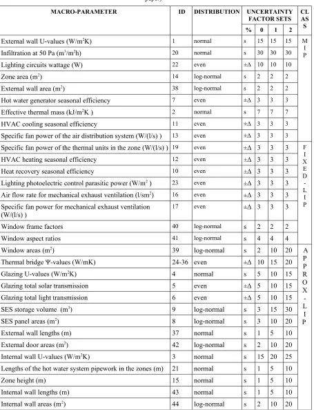
Table 1
Considered macro-parameters, for Case 2, uncertainty distribution and parameters and their typology
(where s indicates the standard deviation as percentage of the mean, ±Δ the lower and upper limit of even distributions as percentages of the mean, MIP the most important parameters, FIXED-LIP the least important parameters to which a fixed value can be attributed and APPROX-LIP the least important parameters definable within ranges – as identified later in the
paper)
MACRO-PARAMETER ID DISTRIBUTION UNCERTAINTY
FACTOR SETS CL AS S
% 0 1 2
External wall U-values (W/m2
K) 1 normal s 15 15 15 M
I P Infiltration at 50 Pa (m3
/m2
h) 20 normal s 30 30 30
Lighting circuits wattage (W) 22 even ±Δ 10 10 10
Zone area (m2
) 14 log-normal s 2 2 2
External wall area (m2
) 38 log-normal s 2 2 2
Hot water generator seasonal efficiency 7 even ±Δ 3 3 3
Effective thermal mass (kJ/m2
K ) 2 normal s 7 7 7
HVAC cooling seasonal efficiency 11 even ±Δ 3 3 3
Specific fan power of the air distribution system (W/(l/s) ) 13 even ±Δ 3 3 3
Specific fan power of the thermal units in the zone (W/(l/s) ) 19 even ±Δ 3 3 3 F I X E D -L I P
HVAC heating seasonal efficiency 12 even ±Δ 3 3 3
Heat recovery seasonal efficiency 10 even ±Δ 3 3 3
Lighting photoelectric control parasitic power (W/m2
) 23 even ±Δ 3 3 3
Air flow rate for mechanical exhaust ventilation (l/sm2) 16 even ±Δ 3 3 3
Specific fan power for mechanical exhaust ventilation (W/(l/s) )
17 even ±Δ 3 3 3
Window frame factors 40 log-normal s 2 2 2
Window aspect ratios 41 log-normal s 4 4 4
Window areas (m2) 39 log-normal s 2 10 20 A
P P R O X -L I P
Thermal bridge Ψ-values (W/mK) 24-36 even ±Δ 10 15 20
Glazing U-values (W/m2
K) 4 normal s 5 10 15
Glazing total solar transmission 5 even ±Δ 5 10 15
Glazing total light transmission 6 even ±Δ 5 10 15
SES storage volume (m3
) 9 log-normal s 3 15 30
SES panel areas (m2) 8 log-normal s 3 10 20
External wall lengths (m) 37 normal s 1 5 10
External door areas (m2
) 42 log-normal s 2 10 20
Internal wall U-values (W/m2K) 3 normal s 15 20 25
Lengths of the hot water system pipework in the zones (m) 21 normal s 1 5 10
Zone height (m) 15 normal s 1 5 10
Internal wall lengths (m) 43 normal s 1 5 10
Internal wall areas (m2
19 thermal zones, served by an HVAC system and an HWS.
The HVAC system is a single duct VAV, powered by an electric ground source heat pump, and equipped with a heat recovery unit, which provides heating and cooling. The HWS is a dedicated hot water boiler fuelled by natural gas. The building is also equipped with a solar hot water system.
The parameters characterising the two building models have been collected and grouped in order to create comparable macro-parameters. For example all the areas of the envelope elements have been grouped and changed together during the simulations. Thus, for Case 1, 56 parameters were considered grouped in 41 macro-parameters and for Case 2, 621 parameters were taken into account and gathered in 44 macro-parameters.
This paper focuses on the results of Case 2, which is considered the more exhaustive one.
Table 1 gives an overview of the considered macro-parameters for Case 2, which are discussed in the following section.
Uncertainty analysis
A computer simulation will be subject to data input errors. Errors can be of two types: systematic and random. The former can be caused by using incorrect data for the input parameters or employing the wrong or incomplete model of the physical process (model inadequacy). The latter are discovered by measuring the same quantity repeatedly under the same conditions and, unlike systematic errors, they can not be attributed to a particular cause.
This study is not focused on the accuracy of the calculation method embedded within SBEM (i.e. the monthly method in BS EN ISO 13790:2008) but it aims to estimate the degree of precision needed in defining the input variables. Thus the uncertainty analysis is focused on the random errors due to measurement errors.
Each data item has been represented through a mean value and another two information items: a minimum and a maximum value (±Δ), or a standard deviation (s) and a probability distribution. This information was obtained from a literature review, where it has been possible to find useful references, or inferred through considerations about the error propagation rules, driven by good sense and experience (Table 1). The assumptions on input uncertainty will have an influence on the results of sensitivity analysis. However it is believed that the methodology provided by the Morris Method is robust enough in that sense, although it may need confirming through additional analyses.
A discussion on the uncertainty relative to the main parameters follows.
Dimensions can be well represented by a log-normal distribution with a standard deviation of 1% of the
mean (Corrado and Mechri 2009). However, this kind of distribution, for small standard deviation, can be well approximated by a normal distribution (Macdonald 2002), which is more manageable. Therefore, dimension uncertainty has been assumed to be normally distributed with a standard deviation of 1%.
The parameters which are product or quotient of dimensions (areas, volumes, frame factors and aspect ratios) have been characterized by a log-normal distribution (Macdonald 2002) with as standard deviation the sum of the standard deviations relative to the parameters involved in the relationship.
Infiltration rate represents a difficult parameter to identify, characterized by high uncertainty. Macdonald (2002) investigated the infiltration of a large series of buildings through simulations and measurements. He concluded that it is possible to represent this parameter with a normal distribution having a standard deviation equal to about 30% of the mean.
To represent the thermal mass of a building, the calculation method uses the effective thermal mass (CM). Its calculation follows the approach in BS EN ISO 13790 (2008); further details can be found in SBEM (2011). It can be represented with the following expression:
C
M=
ρ
∗
C
p∗
t
(3)where ρ is the density of the material (kg/m3), C
p is
the specific heat (J/kgK) and t is the effective thickness of the element (m). The physical variables in the equation can be described by normal distributions. The materials have been considered dry and the effect of the moisture neglected, since that, although it could be significant, is not easy to quantify. Thus it has been possible to consider errors equal to 1%, 3% and 12.5% relatively to density, thickness and specific heat, according to Macdonald (2002). Applying the error propagation rules it has been possible to estimate a global error involved in the datum equal to about 20%. Thus the effective thermal mass has been represented as normally distributed with a standard deviation of 7%.
building they can be used to infer a suitable distribution and a standard deviation. Corrado and Mechri (2009) found the thermal transmittances to be normally distributed, with standard deviation between 12-13% for the external walls, the ground floor and the roof, and equal to about the 3% for the glazing components. In order to generalize these data and after having considered the results provided by Dominguez-Munoz et al. (2010), the values were approximated to 15% for walls, ground floors and roofs and to 5% for the glazing elements.
SBEM follows the methodology explained in the BS EN ISO 10211 (2007) to calculate the effects of thermal bridges. The uncertainties relative to these elements are great and of a different nature. Furthermore very few studies have been done in that sense. An interesting experiment is described by Martin et al. (2012). They compared the results from a calculation done following the BS EN ISO 10211 (2007) method, against the measurements relative to a guarded box experiment. The difference between the two was about 8%. This has been assumed as the possible error involved in the definition of the thermal bridge linear transmittances (Ψ-values). These parameters were represented by an even distribution with Δ = ±10%.
The building services (mainly HVAC and HWS) are described through their seasonal efficiencies. This parameter is a cumulative function of the generator efficiency and the distribution system losses during a typical heating or cooling season. The former has to be input by the assessor, while the latter are characterized by choosing the right class depicted by the CEN classification. Therefore only the uncertainty in generator efficiency was considered. Unfortunately in this case it has not been possible to collect detailed information for each system. However the Standard BS EN 303-5 (1999) states that, for boilers, the efficiency has to be determined within a tolerance of ±3 %. This value has been confirmed by other studies (Heo et al. 2012) and has been considered suitable to represent the uncertainty relative to the seasonal efficiency of generators.
Simulation process
The Morris Method and the Monte Carlo Analysis were implemented in R and Python scripts and applied to the two considered cases.
The work-flow followed the steps listed below: 1. The Morris Method was run according to the
defined uncertainties (Table 1: uncertainty SET-0) and the ee for each input parameter was calculated. 2. For each SBEM output the variables were
classified and ordered following the classification suggested by Garcia Sanchez et al. (2012) defined previously. The MIP and LIP were determined according to the heuristic principle described previously.
3. By comparing the results achieved in the previous step, two general sets of MIP and LIP were defined for each one of the two models. In turn, these general lists were integrated in order to achieve sets of MIP and LIP applicable in both the cases (Table 1).
4. Three Monte Carlo simulations involving variations respectively in all the inputs, MIP and LIP were run, in order to confirm the findings from the former step (Table 1: uncertainty SET-0). 5. The possibility of approximating the LIP was
investigated by dividing these parameters into two groups:
a. FIXED-LIP: coefficients mainly relative to the building services, for which the uncertainties are low and suitable approximated values could be easily found through technical specification or literature (Table 1);
b. APPROX-LIP: physical properties and dimensions of secondary importance for the models, which could be defined within certain ranges (Table 1).
6. The uncertainties relative to the APPROX-LIP were increased as shown in Table 1, obtaining three sets of uncertainty values (table 1: SET-0, SET-1 and SET-2).
7. Monte Carlo simulations for SET-1 and SET-2 were run.
In order to verify the global linear character of the calculation method, the overall standard deviation of the unscaled SBEM output (energy demand, energy consumption, asset rating) provided by the Monte Carlo simulations were compared against the Root Sum of Square (RSS) of the singular effects relative to the parameters:
RSS=
√
∑
i=1n
̄
x
i∗
s
%, i∗
μ
ns,i* (4) wherē
x
i is the input (mean) value of the i-th variable, s%,i is the standard deviation as percentageof the mean of the i-th variable, μ*
ns,iis the μ*i of the
elementary effects for the i-th variable calculated from unscaled inputs and outputs.
RESULT ANALYSIS
(SER) multiplied by 50. SER is derived applying a fixed improvement factor to the emission from the ”reference” building (iSBEM 2012, NCM 2010, SBEM 2011).
In particular only the data achieved for Case 2 will be described since the two cases were in substantial agreement and it is the most exhaustive one.
Morris Method: total energy demand, consumption and building asset rating
The total energy demand (Figure 1) showed linear and monotonic effects for most of the MIP. The LIP behave in a similar manner, with the majority of them having a monotonic influence. Non-linear effects are caused by glass transmittances, internal wall areas, zone areas (Ids: 4, 3 and 14).
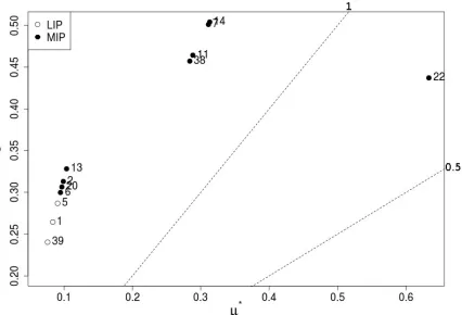
[image:7.595.73.286.75.222.2]All the most important variables relative to the energy consumption (Figure 2) have linear and monotonic effects. Only the thermal transmittance of the external envelope (Id: 1) has a non-linear influence on the output. Considering the least important inputs, these irregular influences are shown by the factors relative to the effective thermal mass, air permeability of the envelope, efficiency of the heat recovery system, glass thermal transmittances, external wall areas, internal wall areas and transmittances (Ids: 2, 20, 4, 38, 44, 3).
Table 2
Case 2, results from ALL, MIP and LIP Monte Carlo simulations (
̄
x
: mean, s: standard deviation)OUTPUT INDEX ALL MIP LIP
Energy demand
s (MJ/m2
) 3.758 3.566 0.872
s/
̄
x
0.016 0.015 0.004RSS (MJ/m2) 3.390 3.336 0.054
Energy consumption
s (MJ/m2
) 4.678 4.658 0.640
s/
̄
x
0.013 0.013 0.002RSS (MJ/m2) 4.313 4.270 0.043
Building asset rating
s 0.581 0.594 0.000
s/
̄
x
0.016 0.016 0.000RSS 0.439 0.434 0.005
The number of non-linearities and non-monotonic effects increases for the building asset rating (Figure 3). All the parameters have at least a non-monotonic effect.
Monte Carlo Analysis: all parameters, MIP and LIP
The simulations involving variations in all the parameters and in the MIP have standard deviations very close to each other, while those regarding only variations in the LIP have values of standard deviation that can be considered negligible. Furthermore the RSS has been shown to be a good approximation of the overall uncertainty defined through the Monte Carlo Analyses (Table 2).
Fundamentally the results just described show that the two main models could be approximated by two meta-models depending only upon the most important parameters without any significant loss of accuracy. Thus these inputs need to be defined with a good degree of precision, while it might be possible consider the others (LIP) in an approximate or simplified way.
[image:7.595.308.524.117.300.2]Figure 2: Case 2, total energy consumption - ee from scaled data
[image:7.595.72.287.590.737.2]Figure 3: Case 2, building asset rating - ee from scaled data
[image:7.595.312.525.591.736.2]Monte Carlo Analysis: increased uncertainties
The incremented uncertainties for the APPROX-LIP, do not lead to any relevant growth of the global uncertainties, especially for Case 2. Comparing the different values of standard deviation, increments are always less than or equal to the 1.5% of the mean (Table 3).
Table 3
Case 2, results from SET-0, SET-1 and SET-2 Monte Carlo simulations (
̄
x
: mean, s: standard deviation)OUTPUT INDEX SET-0 SET-1 SET-2
Energy demand
s (MJ/m2
) 3.758 3.856 4.737
s/
̄
x
0.016 0.016 0.020Energy consumptio n
s(MJ/m2
) 4.678 4.59 4.798
s/
̄
x
0.013 0.013 0.013Building asset rating
s 0.581 0.594 0.629
s/
̄
x
0.016 0.016 0.017Final results
The previous result show that it should be possible to replace the “most exact” set of input data (i.e. in these examples SET-0), with an “approximated” one (i.e. in these examples SET-1 and SET-2), without sensibly affecting the result of the calculation. The possible increment in the percentage errors produced could be calculated as follow:
IE
%,i,n=
2
∗
(
s
%,i,n−
s
%,i,0)
(5)where:
− s%,i,0 is the standard deviation as percentage of the mean, relative to the probability distribution of the i-th SBEM output produced by the “most exact” set of data available; it represents the unavoidable amount of uncertainty;
− s%,i,n is the standard deviation as percentage of the mean, relative to the probability distribution of the i-th SBEM output produced by the “approximated” set of data; it represents the sum of the unavoidable amount and the increment in the uncertainty due to the approximations made. For the two considered cases and approximated sets, the increments in uncertainty are not significant, especially for Case 2 (Table 4).
CONCLUSIONS
A series of sensitivity analyses at the local and global scale were carried out on SBEM, for two well known cases. In particular the Monte Carlo Analysis and the Morris Method were employed, the former as a global method and the latter as a screening method. It was possible to clearly identify the main influences of the model input factors and divide the factors
between most important (MIP) and least important (LIP) (Table 1).
Table 4
Error increments, as percentages of the mean values, for the two cases and the three outputs
CASE OUTPUT SET-1 SET-2
Case 1 Energy demand 0.02 0.05
Energy consumption 0.01 0.02
Building asset rating 0.01 0.03
Case 2 Energy demand 0.00 0.01
Energy consumption 0.00 0.00
Building asset rating 0.00 0.01
At a general level the calculation method showed an almost linear character. In particular, the most influencing factors have linear and monotonic influences on SBEM's outputs. That is also confirmed by the good agreement between the RSS and the overall values of standard deviation returned by the Monte Carlo simulations.
The opportunity to approximate the two main models as meta-models depending only upon the MIP has been demonstrated, as well as the possibility of considering the least important ones in a simplified way. In particular the LIP parameters have been divided, depending on the kind of possible approximations, in least important parameter that are fixed (FIXED-LIP in Table 1) and least important parameters that can be approximated within defined ranges (APPROX-LIP in Table 1). In both cases studied, considering increased uncertainties for the identified LIP produces negligible increments in the standard deviations and errors relative to the model responses.
These results open the way to further simplifications in the input procedure in iSBEM. In particular simplified input methods could be implemented for some of the less important parameters, considering the determined tolerable increased uncertainties. For example the window area could be specified as a percentage of the wall as high, medium or low and the internal wall areas could be automatically calculated as functions of the internal wall length and height of the zone, since any possible irregular shapes should not produce significant errors.
The Morris Method can effectively and efficiently identify the characteristics and the extent of the influences for the input parameters and screen them. The Monte Carlo Analysis is a good method for assessing the effects of approximations on groups of parameters. It should be noticed that for calculations and models for which the majority of the most important parameters have linear or monotonic effects, the results of the Monte Carlo Analysis could be well approximated by the Root Sum Squares of the singular effects involved, saving computational time.
The method described in this paper is flexible and not software dependent and in addition to guiding the design of user interfaces, the approach could be used to develop guide lines for all the data input and collection processes. For example the training of the assessors could be structured depending on the tolerable uncertainty values resulting from the analysis, so that the focus would be proportionally distributed depending on the influence and importance of each input parameter.
It should be said that the design and definition of procedures and tools involved in the analysis of a multitude of buildings should be based on relevant statistically results. Thus the methodology in this paper should be applied to a statistically relevant sample of buildings to confirm the results presented. Furthermore it is recognized that there is a significant gap between predicted and real data. In future developments a similar approach could be adopted in calibration studies employing metered data in order to see how and to what extent different parameters contribute to the mismatch between predictions and reality.
Finally, the assumptions made in undertaking uncertainty analysis in terms of the assumed distribution, standard deviations and uncertainty ranges could have an influence on the output of the Morris Method and Monte Carlo Analysis. However this issue can easily be overcome, by defining suitable uncertainty structures for the data, in agreement with the various parties involved.
REFERENCES
Alam F M, McNaught K R, and Ringrose T J, 2004. Using Morris' Randomized OAT Design as a Factor Screening Method for Developing Simulation Metamodels.International Journal of Enterprise Information Systems, 2(4), pp38-57. BS EN ISO 303-5:1999. Heating boilers - Part 5:
Heating boilers for solid fuels, hand and automatically fired, nominal heat output of up to 300 kW - Terminology, requirements, testing and marking.
BS EN ISO 10211:2007.Thermal bridges in building construction - Heat flows and surface temperatures - Detailed calculations.
BS EN ISO 13790:2008. Energy performance of buildings - Calculation of energy use for space heating and cooling.
Campolongo F and Braddock R, 1999. The Use of Graph Theory in the Sensitivity Analysis of the Model Output: a Second Order Screening Method. Reliability Engineering & System Safety, 64(1), pp1-12.
Campolongo F, Cariboni J and Saltelli A, 2007. An Effective Screening Design for Sensitivity Analysis of Large Models. Environmental Modelling & Software, 22(10), pp1509-1518. Corrado V and Mechri H E, 2009. Uncertainty and
Sensitivity Analysis for Building Energy Rating. Journal of Building Physics, 33(2), pp125-156. Cropp, R A and Braddock, R D. The New Morris
Method: an efficient second-order screening method.
Reliability Engineering & System Safety, 2002, 78, pp77-83
Dominguez-Munoz F, Anderson B, Cejudo-Lopez J M, and Carrillo-Andres A, 2010. Uncertainty in the Thermal Conductivity of Insulation Materials. Energy and Buildings, 42(11), pp2159-2168.
Garcia Sanchez D, Lacarrière B, Musy M and Bourges B, 2012. Application of Sensitivity Analysis in Building Energy Simulations: Combining First and Second Order Elementary Effects Methods. Energy and Buildings.
http://dx.doi.org/10.1016/j.enbuild.2012.08.048. Heo Y, Choudhary R and Augenbroe G A, 2012.
Calibration of Building Energy Models for Retrofit Analysis under Uncertainty. Energy and Buildings, 47, pp550-560.
iSBEM 2012, A User Guide to iSBEM, Building Research Establishment, Garston.
Macdonald I A, 2002. Quantifying the Effects of Uncertainty in Building Simulation. PhD thesis, University of Strathclyde, Glasgow.
Martin K, Campos-Celador A, Escudero C, Gomez I and Sala J M, 2012. Analysis of a Thermal Bridge in a Guarded Hot Box Testing Facility. Energy and Buildings, 50, pp139-149.
Morris, M D. Factorial sampling plans for preliminary computational experiments. Technometrics, 1991, 33(2), pp161–174.
NCM 2010, National Calculation Methodology (NCM) modelling guide (for buildings other than dwellings in England and Wales).
SBEM 2010, Volume 3: C++ code.