Numerical identification of a variable parameter in 2d elliptic boundary value problem by extragradient methods

Rochester Institute of Technology

RIT Scholar Works

Theses Thesis/Dissertation Collections

6-17-2013

Numerical identification of a variable parameter in

2d elliptic boundary value problem by

extragradient methods

Selin Sariaydin

Follow this and additional works at:http://scholarworks.rit.edu/theses

This Thesis is brought to you for free and open access by the Thesis/Dissertation Collections at RIT Scholar Works. It has been accepted for inclusion in Theses by an authorized administrator of RIT Scholar Works. For more information, please [email protected].

Recommended Citation

Numerical Identification of a Variable

Parameter in 2D Elliptic Boundary

Value Problem by Extragradient

Methods

by

Selin Sariaydin

A Thesis Submitted in Partial Fulfillment of the Requirements

for the Degree of Master of Science in Applied Mathematics

Department of Mathematics, College of Science

Rochester Institute of Technology

Rochester, NY

June 17, 2013

Advisor: Dr. Akhtar A. Khan

Committee: Prof. Patricia Clark

Dr. Baasansuren Jadamba

Abstract

This work focuses on the inverse problem of identifying a variable parameter

in a 2-D scalar elliptic boundary value problem. It is well-known that this

in-verse problem is highly ill-posed and regularization is necessary for its stable

solution. The inverse problem is studied in an optimization framework, which

is the most suitable framework for incorporating regularization. This

optimiza-tion problem is a constrained optimizaoptimiza-tion problem where the constraint set

is a closed and convex set of the admissible coefficients. As an objective

func-tional, we use both the output least squares and modified output least squares

functionals. It is known that the most commonly used iterative schemes for

such problems require strong monotonicity of the objective functionals

deriva-tive. In the context of the considered inverse problem, this is a very stringent

requirement and is achieved through a careful selection of the regularization

parameter. In contrast, extragradient type methods only require the derivative

of the objective functional to be monotone and this allows a greater

flexibil-ity for the selection of the regularization parameter. In this work, we use the

finite element method for the discretization of the inverse problem and apply

Dedicated to my parents

Hava and Aziz Sariaydin

Acknowledgement

I would like to express my deepest gratitude to my family for supporting me

throughout my entire education most recently, the completion of my masters.

I would like to thank my advisor, Dr. Akhtar Khan for his guidance. Dr. Khan

provided access to an extensive set of resources including unique courses, and

a chance to meet with great mathematicians from around the world.

I also consider myself very lucky to work with an excellent research group.

In particular, I would like to thank Brian Winkler who was willing to spend his

valuable time to overcome computational difficulties and Nate Bush who was

always ready to help. Special thanks to Noorullah Maqsoodi, who was willing to

study with me for hours. I owe my deepest gratitude to my good friend, Ashley

Zanca, who was always there to support and encourage me to do better.

I also want to thank International Institute of Education, Turkish Fulbright

Commission, and the School of Mathematical Sciences at RIT for the financial

grant and the constant support.

Many thanks to my committee members: Patricia Clark, Baasansuren Jadamba,

Contents

1 Introduction to Inverse Problems 1

1.1 Problem Formulation . . . 2

1.2 Variational Problem . . . 3

1.3 Solution Differentiability . . . 6

1.4 An Optimization Framework of the Inverse Problem . . . 8

1.4.1 Output Least-Squares . . . 8

1.4.2 Modified Output Least-Squares . . . 9

1.4.3 Regularization . . . 9

2 The Finite Element Method for the Inverse Problem 11 2.1 The Galerkin Method . . . 12

2.2 Discrete Formulas for the OLS . . . 15

2.3 Discrete Formulas for the MOLS . . . 16

2.4 Discrete Formulas for the Regularization . . . 17

3 Extragradient Methods 18 3.1 Literature Review . . . 18

3.2 The Projection Method . . . 20

3.3 Extragradient Methods . . . 22

CONTENTS vi

3.3.2 Solodov-Tseng Method . . . 30

3.3.3 Improved Goldstein’s Method . . . 32

3.3.4 Hyperplane Method . . . 36

4 Performance Analysis 38

5 Background Material 47

List of Figures

3.1 Geometry of Hyperplane Extragradient Method . . . 28

3.2 Solution by Second Modified Version of Marcotte . . . 31

3.3 Solution by Solodov-Tseng Method . . . 33

3.4 Solution by Improved Goldstein’s Method . . . 35

3.5 Solution by Hyperplane Method . . . 37

4.1 Reduction Rule for Solodov-Tseng Method . . . 39

4.2 Reduction Rule for Improved Improved Goldstein’s Method . . . . 39

4.3 Performance Analysis of OLS . . . 41

4.4 Performance Analysis of MOLS . . . 42

4.5 Solution by Different Regularization Parameters . . . 44

4.6 ComputedAfor Various Extragradient Methods . . . 46

List of Tables

4.1 α performance by Khobotov . . . 40

4.2 α performance by MOLS . . . 40

4.3 α performance by OLS . . . 42

4.4 Regularization parameter,ε, performance . . . 43

Chapter 1

Introduction to Inverse Problems

In the following chapter, we give a brief introduction to inverse problems. The

following phrase adequately defines inverse problems:

In inverse problems one seeks unknown causes based on observation of their

effects. On the other hand, for the direct problem, one seeks effects based on

suffi-cient knowledge about the causes.

We emphasize that the inverse problems have quite different behaviour than

the direct problems. Due to their special properties, most inverse problems

areill-posed. In 1932, J. Hadamard defined the generic properties of problems

which arise from physical and natural phenomena. Based on Hadamard’s

def-inition, a mathematical problem is calledwell-posed if it has the following

fea-tures:

1. Existence:For a suitable data set, the problem is solvable.

2. Uniqueness:The solution is unique.

3. Stability:The solution depends continuously on the data.

Following the above criteria, a problem is termed as ill-posed if it fails any of

1.1. Problem Formulation 2

problems is the violation of the third condition, that is, the case in which the

solution does not depend continuously on the data.

In this work, we focus our attention to the study of inverse problems of

iden-tifying physical parameters in 2-D elliptic partial differential equations (PDE).

Inverse problems have been the subject of several papers [1, 11, 12, 13, 14, 15] .

1.1

Problem Formulation

We focus on the elliptic inverse problem of estimating the coefficienta in the

elliptic boundary value problem (BVP):

−∇·(a∇u(x)) = f inΩ, (1.1a)

u = 0 on∂Ω. (1.1b)

This problem is a particular case of the more general following BVP

∇·(a∇u(x,t)) =B(x)∂u

∂t +C(x,t)

which models a confined inhomogeneous isotropic aquifer. Here,urepresents

the piezometric head, a the transmissivity, C(x,t) the recharge, and B(x) the

storativity of the aquifer. It is commonly observed that aquifers tend to bethin

relative to their horizontal extent and thus a natural simplification is the

as-sumption that the transmissivity varies little with depth, so that the ground

wa-ter flow in these cases can be viewed as essentially two dimensional, and we can

takex= (x₁,x₂)in a two dimensional space. If the flow of the water has reached a steady state and we assume for simplicity thatC=0,then one can obtain (1.1).

1.2. Variational Problem 3

1.2

Variational Problem

In this work, we will use finite element methods to solve the inverse as well as

the direct problem. As it is well-known, for finite element methods, the BVP

should be converted into the so-called the variational form.

In this section, our objective is to introduce the variational form of (1.1). For

this, we begin by recalling the product rule in multiple dimensions:

∇·(v∇u) = ∇·

 v   ∂u ∂x ∂u ∂y     = ∇·     v∂u

∂x

v∂u

∂y     = ∂ ∂x v∂u

∂x

+ ∂

∂y

v∂u

∂y

= ∂v

∂x ∂u ∂x+v

∂2u ∂x2+

∂v ∂y

∂u ∂y+v

∂2u ∂y2

= ∂v

∂x ∂u ∂x+

∂v ∂y

∂u ∂y+

v

∂2u ∂x2+

∂2u ∂y2

= ∇v·∇u+v∆u.

Now, integrating both sides over Ω and applying the divergence theorem

gives Green’s identity:

∇·(v∇u) = ∇v·∇u+v∆u

⇒

Z

Ω

∇·(v∇u) = Z

Ω

∇v·∇u+ Z

Ω

v∆u

⇒

Z

∂Ω

v∇u·n = Z

Ω

∇v·∇u+ Z

Ω

v∆u.

Therefore, by denoting∇u·nwith ∂u

∂n, we get

−

Z

∂Ω

v∆u= Z

Ω

∇v·∇u− Z

∂Ω

v∂u

∂n (1.2)

To write (1.1) into a variational form, we multiply it by an arbitraryv∈H₀1(Ω)

1.2. Variational Problem 4

we deduce the following variational form of (1.1): Findu∈H₀1(Ω)such that Z

Ω

a∇u·∇v= Z

Ω

f v for allv∈H₀1(Ω). (1.3)

It is convenient to express this variational problem in terms of a trilinear

form. For this, we writeV =H₀1(Ω) and B= L∞(Ω). Here, B is the coefficient

space. We define the set of all admissible coefficients as follows:

A={a∈L∞₍

Ω) : k0≤a≤k1},

wherek₁>k₀>0are given.

We then defineT :B×V×V →_Rby

T(a,u,v) =

Z

Ω

a∇u·∇v.

Clearly,T is symmetric inuandv.

We further note that

T(a,u,v) =

Z

Ω

a∇u·∇v

≤ max

a∈Ω|a|k∇ukL2(Ω)k∇vkL2(Ω)

≤ k1k∇uk_L2_(Ω)k∇vk_L2_(Ω)

where the Cauchy-Schwarz inequality has been used. Forw∈V,we have

k∇wk2_L2_(Ω) =

Z

Ω

∇w·∇w

≤

Z

Ω

w2+∇w·∇w

= kwk2_H1_(Ω) and consequently

T(a,u,v)≤ kakBkukVkvkV,

1.2. Variational Problem 5

For the ellipticity of the trilinear formT,we recall the Poincar´e’s inequality:

There exists a positive constantC,depending on the domainΩ,such that

r_Z

Ω

∇u·∇u≥Ckuk_H1_(Ω) for allu∈H₀1(Ω). (1.4) Consequently,

T(a,u,u) =

Z

Ω

a∇u·∇u

≥ k₀

Z

Ω

∇u·∇u

≥ k₀Ckuk_V2

implying that

T(a,u,u)≥αkuk_V2 for allu∈V, a∈A,

whereα =k0C>0.

This variational equation (1.3) can also be expressed as

T(a,u,v) =m(v) for allv∈V,

wheremis the bounded linear functional onV defined by

m(v) =

Z

Ω

f v.

The above arguments can easily be extended to the BVP with mixed

bound-ary conditions such as:

−∇·(a∇u) = f inΩ,

u = 0 onΓ1,

a∇u(x)·ν = g onΓ2

where∂Ω=Γ1∪Γ2.

For this case, the underlying Hilbert space becomes:

1.3. Solution Differentiability 6

The variational form, by using standard arguments, becomes:

Z

Ω

a∇u·∇v= Z

Ω

f v+

Z

Γ2

vg for allv∈V.

Therefore, in an attempt to write it in the form (1.3), the trilinear form

re-mains the same as for (1.1) but the functionalmhas to be modified to:

m(v) =

Z

Ω

f v+

Z

Γ2 vg.

1.3

Solution Differentiability

The existence and uniqueness of solution to the variational form of the problem

can be given by the Lax-Milgram theorem that can be found in the appendix.

Therefore, we can define F :A→V such that F(a) =u is the solution of the variational problem.

Lemma 1.3.1. For eacha∈A,u=F(a)satisfies

kukV ≤α−1kmkV∗.

Proof. Using the V-ellipticity of the trilinear form:

T(a,u,v) =m(v) for allv∈V

⇒ T(a,u,u) =m(u)

⇒ αkuk_V2 ≤ kmkV∗kukV

⇒ kuk_V ≤α−1kmkV∗.

Theorem 1.3.2. The solution operatorF satisfies the following conditions:

kF(a)−F(b)kV ≤

β αkF(

a)kVkb−akB,

kF(a)−F(b)kV ≤

β αkF(

b)kVkb−akB,

kF(a)−F(b)kV ≤

β α2k

1.3. Solution Differentiability 7

The following result gives information regarding the differentiability of the

solution map:

Theorem 1.3.3. For eachain the interior ofA, the operatorF is differentiable at

a, andδu=DF(a)δais the unique solution to the variational problem.

T(a,δu,v) =−T(δa,u,v) for allv∈V, (1.5)

whereu=F(a). Moreover,

kDF(a)k ≤ β

αk

ukV,

and hence, for allain the interior ofY,

kDF(a)k ≤ β

α2kmkV

∗.

Now, we can also show that F is infinitely differentiable. We will just state

the second derivative.

Theorem 1.3.4. For eachain the interior ofA, the operatorF is twice-differentiable

ata, and

δ2u=D2F(a)(δa1,δa2)

is the unique solution to the variational problem.

T(a,δ2u,v) =−T(δa2,DF(a)δa1,v)−T(δa1,DF(a)δa2,v) for allv∈V. (1.6)

Moreover,

D2F(a)≤

2β2

κ2 kF(a)kV ≤

2β2 κ3 kmkV

∗.

1.4. An Optimization Framework of the

Inverse Problem 8

1.4

An Optimization Framework of the

Inverse Problem

We recall that there are two primary approaches for solving the inverse

prob-lem of identifying the coefficient,a. The first approach reformulates the inverse

problem as an optimization problem and then employs some suitable method

for the solution. The second approach views (1.1) as a hyperbolic partial

differ-ential equation ina.

In this work, we pose the considered inverse problem as an optimization

problem whose numerical solution is an approximation of the coefficient to be

identified. As is well-known, the inverse problem is ill-posed, and some type of

regularization is necessary. Since this is more easily accomplished in the

opti-mization setting, this class of methods has been the subject of most of the

re-search.

In the following, we briefly outline some of the main approaches available in

the literature for the inverse problems.

1.4.1

Output Least-Squares

A common approach for solving parameter identification problems is the

out-put least-squares (OLS) approach. Applied to the elliptic inverse problem of

findingain (1.1), the OLS approach minimizes the functional

J1(a) =ku(a)−zk2, (1.7)

wherezis the data (the measurement ofu),k · kis a suitable norm andusolves the BVP or its variational form: Findu∈H₀1(Ω)such that

Z

Ω

a∇u∇v= Z

Ω

1.4. An Optimization Framework of the

Inverse Problem 9

1.4.2

Modified Output Least-Squares

For the scalar inverse problem, a variation on the OLS approach was proposed

independently by Knowles [22]. They replaced theL₂norm by the coefficient-dependent energy norm:

J₂(a) = 1

2 Z

Ω

a∇(u(a)−z)·∇(u(a)−z). (1.9)

In [12], the following extension of the modified output least-squares (MOLS)

functional was introduced:

J₂(a) =1

2T(a,u−z,u−z),

whereT is a general trilinear form.

1.4.3

Regularization

Regularization is a very common technique to solve ill-posed problems or

pre-vent overfitting. Regularization has an impact role in uniqueness. It can make

a non-unique problem become a unique problem. Moreover, it is important to

choose regularization parameter correctly since choosing a poor regularization

parameter can create a different problem. We can choose one of the following

forms for the regularization:

L2norm: Rε(a) =

ε

2||a||

2

L2 (1.10)

H₁semi−norm: R_ε(a) = ε

2||∇a||

2

L2

H1norm: Rε(a) =

ε

2(||a||

2

L2+||∇a||

2

L2)

whereR_ε(a)is the regularization.

The basic idea is to add a suitable functional to penalize numerical features

1.4. An Optimization Framework of the

Inverse Problem 10

significant importance on smoothing the data, hence it is very critical to choose

the right regularization parameter. In the Performance Analysis chapter, we

in-clude some figures that show how the computed solution can differ depending

on the regularization parameter.

Now, we can define the constrained optimization problem as following:

min

a∈A{J(a) +Rε(a)} (1.11)

whereε is the regularization parameter andJ(a)is either OLS,J1(a), or MOLS,

J2(a).

We will solve the inverse problem by writing the minimization problem as a

variational inequality of findinga∗∈Asuch that

hDJ(a∗) +DR_ε(a∗),a−a∗i ≥0 ∀a∈A,

Here, OLS is non-convex and the following relaxed-monotonicity holds [21]:

hDJ₁(x)−DJ₁(y),x−yi ≥ −m||x−y||2, ∀x,y∈A,m>0

For a sufficiently smooth and strongly convex regularization termR_ε, we have

hDR_ε(x)−DR_ε(y),x−yi ≥εm0||x−y||2, ∀x,y∈A,m0>0

To use extragradient methods which are convergent under strong

mono-tonicity, we need to assume that

−m+εm0=m1>0

Whilem₀ =1and mis usually fixed, regularization parameter, ε, is required to

be large for convergence [26]. It is also useful to state that ifε is too large, then

we will have an over-regularized solution and choosing a smallε will lead to an

Chapter 2

The Finite Element Method for the

Inverse Problem

In this chapter, we will give the basic idea of the finite element method (FEM).

To obtain the finite element method for the two dimension problem, we will use

the weak form of the boundary value problem. Then, we will apply the Galerkin

method to the weak form of the problem. Finally, we will define the finite

el-ement spaces which is the most important difference from the one dimension

case. The details can be found in [9].

Recall the weak form of the 2D problem:

Z

Ω

a(x)∇u·∇v= Z

Ω

f v f or all v∈V. (2.1)

Now we can define the bilinear form ofa(·,·)as the following: a(u,v) = (f,v)

where

a(u,v) =

Z

Ω

a(x)∇u·∇v

and

(f,v) =

Z

Ω

2.1. The Galerkin Method 12

Hence, the problem is to findu∈V such that

a(u,v) = (f,v) ∀v∈V (2.2)

2.1

The Galerkin Method

The Galerkin method approximates to the solution accurately when energy

in-ner product is used and the variational form of the BVP computes the value of

a(u,v)for all v∈V. Solving KU =F matrix-vector equation gives the best ap-proximation touwhereKis the stiffness matrix andF is the load vector.

LetVn be finite dimensional subspace ofV and let{φ1,φ2,· · ·,φn}be a basis

forV_n. Then (2.2) is defined as the Galerkin problem [9] :

u_n= n

∑

j=1

U_jφj (2.3)

Then, we can rewrite the Galerkin problem as

a(un,φi) = (f,φi) f or i=1,2,3, ...,n (2.4)

Using (2.3), we have

a( n

∑

j=1

U_jφj,φi) = (f,φi)

⇒

n

∑

j=1

a(φj,φi)Uj= (f,φi) f or i=1,2,3, ...,n

⇒KU =F (2.5)

whereKis the stiffness matrix and f is the load vector, that is:

K_{i j} =a(φj,φi) and fi= (f,φi) i,j=1,2,3, ...,n

2.1. The Galerkin Method 13

FEM can be seen as a Galerkin method when a particular subspace and its

basis are chosen. If the coefficient matrix is dense, solving the linear system and

finding the orthogonal basis are difficult since the computations require

exten-sive time. However, FEM uses a basis that leads to a sparse coefficient matrix.

Since the sparse matrix has mostly zero entries, solving the linear system will be

less time-consuming.

Another interpretation of the Galerkin method can be defined as in an

ab-stract setting the variational problem of findingu∈V such that

a(u,v) = f(v) ∀v∈V

is given by

J(u) = 1

2a(u,u)−f(u).

The problem is findu∈V such that

min u∈VJ(u)

Instead we solve the problem

min w∈WJ(w)

whereW is a finite dimensional subspace ofV. This approach is called the Ritz

Method.

Let{w₁,· · ·,w_n}be a basis forW. Then, we have

w=

n

∑

i=1

2.1. The Galerkin Method 14

Therefore,

J(w) = 1

2a(w,w)−f(w)

= 1

2a( n

∑

j=1

U_jw_j, n

∑

i=1

U_iw_i)−f( n

∑

i=1

U_iw_i)

= 1

2 n

∑

i=1

n

∑

j=1

a(w_j,w_i)U_jU_i−

n

∑

i=1

f(w_i)U_i

= 1

2U·KU−F·U

whereKis the stiffness matrix andF is the load vector.

Therefore, the problem is to findU ∈Rnsuch that J(U) = 1

2 <U,KU >−<F,U >

is minimized.

The gradient ofJcan be defined as

∇J(U) =KU−F

and∇J(U) =0then the linear system is given by

KU =F

Recall the stiffness matrix,Khas the following form:

K_{i j} =a(φj,φi) = n

∑

i=1

a(φj,φi) (2.6)

Then, the stiffness matrix can be written as

K_{i j}=

Z

Ω

k∇φi·φj i,j=1,2,· · ·,n

[10] includes details about the theory and some examples to show how to

com-pute the stiffness matrix,K.

The load vector has the following form:

F_i = hf,φii =

Z

Ω

2.2. Discrete Formulas for the OLS 15

2.2

Discrete Formulas for the OLS

We will need discrete analogue of the OLS functional to solve the inverse

prob-lem numerically, so we will define the finite eprob-lement solution operator asF :

Rm→Rnmapping a coefficienta∈Amto the approximate solutionu∈Umwhere

m=n+2. ThenF(A) =U whereUis defined as

K(A)U=F

K(A), the stiffness matrix, has the following form:

K_{i j} =

Z

Ω

k∇φj·∇φi i=1,2,· · ·,n

and the load vector has the following form:

F_{i j} =

Z

Ω

fφi i=1,2,· · ·,n

It is also important to know that the tensor is defined as

T_{i jk}=

Z

Ω

ψk∇φi·∇φj i,j=1,2,· · ·,n, k=1,2,· · ·,m

Therefore, the stiffness matrix can be defined by

K(A)i j=Ti jkAk

Now, we can discretize the system using the basis functions forAn,{ψ1,ψ2,· · ·,ψm}

and forU_n,{φ1,φ2,· · ·,φn}. Thus,

a=

m

∑

i=1

A_iψi

u=

n

∑

i=1

Uiφi

Therefore, the discrete form of the OLS can be stated as [15]

J1(A) =

1

2.3. Discrete Formulas for the MOLS 16

where the mass matrixM∈_Rn×n_is

Mi,j=

Z

Ω

φiφjdx, i,j=1,2,· · ·,n

We will also need the gradient of the objective functional, that is:

∇J1(A) =−L(U)TK(A)−1M(U−Z)

where the the adjoint-stiffness matrixLsatisfies the following condition:

L(U)A=K(A)U, ∀A∈_Rn, U∈_Rn

We can also compute the hessian matrix by using similar notation:

∇2J1(A) =L(U)TK(A)−1MK(A)−1L(U) +L(K(A))−1M(U−Z)TK(A)−1L(U)

+L(U)TK(A)−1L(K(A))−1M(U−Z))

2.3

Discrete Formulas for the MOLS

Define an objective functionJ₂:Rm→Ras

J₂(A) =1

2 Z

Ω

a(∇u−∇z)·(∇u−∇z)

whereuis defined asF(A) =Uandzis the measurement of the exact solutionu

of the original problem.

The discrete modified output least squares can be written as

J2(A) =

1

2(U−Z)·K(A)(U−Z)

and it follows that

∇J2(A) =−

1 2L(U)

T_U+1 2L(Z)

T_Z

and the hessian can be defined as

∇2J2(A) =L(U)TK(A)−1L(U)

The details about the derivation of the discrete form for the OLS and MOLS

2.4. Discrete Formulas for the Regularization 17

2.4

Discrete Formulas for the Regularization

The discrete formulas for the regularization,R_ε(a)are as the following:

L2norm: Rεα =

ε

2A T_MA˜

H1 semi−norm: Rεα =

ε

2A T_KA˜

H1norm: R_εα =ε

2A

T_{(M˜ +K˜)A}

Chapter 3

Extragradient Methods

3.1

Literature Review

In 1976, the first extragradient method was introduced by Korpelovich [23]. To

describe the framework of her contribution, let f be a convex-concave function

with a non-empty set of saddle points onPQ, wherePandQare convex closed

subsets of finite-dimensional space. She assumed that the function f is

differ-entiable and f0satisfied the Lipschitz condition with some constantL. Her work

was motivated by the fact that the gradient method with constant stepsize

un-der those conditions is in general known not to converge to the set of saddle

points. As a remedy, she proposed a scheme defined by recursive relations by

projecting twice on the underlying convex sets and proved the convergence of

the generated sequence to some saddle point. She showed that in a particular

case, when f is the Lagrange function of linear programming problem, the rate

of convergence is exponential.

In 1987, Khobotov [18] presented a modification of the extragradient method

proposed by Korpelovich [23] for solving variational inequalities defined for

con-3.1. Literature Review 19

vergence of the proposed scheme and discussed interesting applications in

ar-eas such as convex optimization, min-max theory and game theory.

Marcotte [24] strengthened the method proposed by Khobotov by providing

some useful strategies for its implementation.

In 1996, Solodov and Tseng introduced a modification to projection-type

methods by using a strongly monotone operator.

In addition, a nice geometric interpretation of the extragradient methods

was proposed in [16, 17]. The method is continuous and satisfies a certain

gen-eralized monotonicity assumption (e.g., it can be pseudomonotone). Later, this

method was developed by Solodov and Svaiter [29]. The idea of the method is to

construct an appropriate hyperplane which strictly separates the current iterate

from the solutions of the problem. This procedure requires a single projection

onto the feasible set and employs an Armijo-type linesearch along a feasible

di-rection. Then the next iterate is obtained as the projection of the current iterate

onto the intersection of the feasible set with the halfspace containing the

so-lution set. The method is globally convergent to a soso-lution of the variational

inequality problem.

He [30] implemented an extension of the Goldstein’s projection method which

was later improved in [31]. This method provided an easily-implementable

Armijo-type strategy using the scaling parameters.

Popov [27] proposed a regularized extragradient method for solving a

varia-tional inequality with monotone Lipschitz operator. The inequality was

consid-ered in a finite-dimensional Euclidean space. The method allowed to construct

an iterative process that converged to a solution of minimal norm. The

peculiar-ity of the proposed process is that the descent direction at every iteration step is

calculated only once (not twice as in the standard extragradient method). In the

case when the inequality is unsolvable, it was shown that the proposed method

3.2. The Projection Method 20

approximation” (in the sense suggested by the author) to the given problem.

Recently, Y. Censor, A. Gibali, S. Reich [8] proposed two extensions of the

well-known extragradient method for variational inequality problems. The first

extended method replaced the second orthogonal projection in the original

ex-tragradient method by a specific subgradient projection and the second extended

method allowed projections onto the members of an infinite sequence of

sub-sets which epi-converges to the feasible set of the VIP. Both methods were shown

to be convergent under suitable conditions.

In [7], the authors presented a subgradient extragradient method for solving

variational inequalities in Hilbert space and proved the weak-convergence of

the method.

Extragradient methods have been well-studied in various papers.( see [2, 3,

4, 5, 25, 33, 34, 35])

3.2

The Projection Method

LetJ :A→H be a continuous function and consider the variational inequality problem of findingx∗such that

x∗∈A hJ0(x∗),x−x∗i ≥0,∀x∈A (3.1)

whereAis a nonempty convex set. One of the most common methods is to solve

the variational inequality problem by using the projection algorithm:

xk+1=P_A(xk−αJ0(xk)) (3.2)

whereP_A(·)is the orthogonal projection map ontoA, and α is the step length.

Here, projection method uses the gradient of the objective function as the

3.2. The Projection Method 21

x∗=PA(x∗−αJ0(x∗)) (3.3)

Lemma 3.2.1. LetAbe a closed convex subset of Hilbert space. LetJ0be Lipschitz

continuous and strongly monotone inA, that is:

||J0(x)−J0(y)|| ≤ L||x−y|| ∀x,y∈A (3.4)

hJ0(x)−J0(y),x−yi ≥ l||x−y||2 ∀x,y∈A (3.5) Then, the projection method(3.2)converges to a solution of (3.1)ifα ∈(0,2l/L2)

where l is the monotonicity constant andLis the Lipschitz constant.

Proof. We can prove the convergence of the projection method using

contrac-tive properties of the operator. Setx→xk+1−αJ0(xk+1)andy→x∗−αJ0(x∗)in

||P_A(x)−P_A(y)|| ≤ ||x−y||for all x,y∈Hthen:

kxk+1−x∗k2 = kPA(xk−αJ0(xk)−PA(x∗−αJ0(x∗)k2

≤ k(xk−αJ0(xk))−(x∗−αJ0(x∗))k2

= kxk−x∗||2−2αhJ0(xk)−J0(x∗),xk−x∗i+α2kJ0(xk)−J0(x∗)k2

≤ (1−2αl+α2L2)kxk−x∗k2,

which due to the assumption thatα < 2l

L2 ensures that

(1−2αl+α2L2)<1

and consequently, we get that the sequence{xk}converges strongly tox∗.

Projection methods are easy to implement. However, there are many

draw-backs of the iterative algorithm. First and foremost,J0is required to be strongly

monotone and Lipschitz continuous which are very powerful criteria to meet.

3.3. Extragradient Methods 22

know the values ofl,Land failure to choose these constants may lead slow

con-vergence or not concon-vergence at all.

A mapping is coercive withc`=1/L2if it is strongly monotone and Lipschitz continuous and any coercive mapping is monotone and Lipschitz withL=1/c`

such that

hJ0(x)−J0(y),x−yi ≥0, ∀ x,y∈A.

The projection algorithm converges for coercive variational inequalities which

relaxes the requirement onJ0 [32]. However, the problem of choosing the right

initial step length still exists since it still depends on the Lipschitz constant.

One modification can be to estimate Lipschitz constant by introducing

adap-tivity in the projection method by Armijo line search. This modification allows

step length to vary at each iteration and relaxes the requirements onJ0. Another

modification can be projecting twice at each iteration which is called

extragra-dient methodsthat is first introduced by Korpelevich [23].

3.3

Extragradient Methods

The focus of this research is to implement the extragradient methods for the

el-liptic boundary value problem which relaxes the convergence requirements. In

this section, we will give brief introduction and convergence analysis for some

extragradient methods. Then, we will discuss computational aspects of the each

method and identify a variable parameter in 2D elliptic boundary value

prob-lem by these methods.

The projection methods requires strong theoretical properties for

conver-gence that are not easy to verify in practice. Korpelevich [23] proposes a

modi-fied version to the projection method to relax these requirements. Let us recall

3.3. Extragradient Methods 23

¯

xk=PA(xk−αJ0(xk)) (3.6)

Here, the gradient of the pointx¯kwill be the direction for the new point. Overall,

the basic idea is to project twice at each iteration to find the solution of (3.1) for

givenx0∈Asuch that

¯

xk = P_A(xk−αJ0(xk)) (3.7a)

xk+1 = PA(xk−αJ0(x¯k)), (3.7b)

whereα is the constant step length.

Theorem 3.3.1(Korpelevich, [23]). LetAbe a closed convex subset ofRnandA∗

be a nonempty set of solutions of (3.1).J0is monotone operator inAand Lipschitz

continuous withα∈(0,1/L)whereLis the Lipschitz constant, thenxkthat defined

by (3.7)converges to some solution of the variational inequality,x∗∈A∗.

Choosing the right step length plays a vital role for convergence as it is stated

in the Theorem 3.3.1. SinceLis unknown, it is difficult to determine a suitable

step length,α. Placing a small value for step length may lead slow convergence.

However, the method might not converge if the step length is too large.

Then, Khobotov, [18] proposed a modification to choose step length which

is changingα at each iteration:

¯

xk = P_A(xk−αkJ0(xk)) (3.8a)

xk+1 = P_A(xk−αkJ0(x¯k)). (3.8b)

IfJ0(x¯k) =0, thenx¯kis a solution to the variational problem of (3.1) and here

α_ksatisfies the following inequality:

0<αk≤min

¯

α,ε ||x

k_−x¯k_||

||J0(xk_)−J0_(x¯k_||

3.3. Extragradient Methods 24

whereα¯ is the maximum value forα andε∈(0,1). Khobotov states the

fol-lowing theorem which is a very important for convergence analysis of the

extra-gradient method.

Theorem 3.3.2(Khobotov, [18]). LetAbe a closed convex subset ofRnandA∗be

a nonempty set of solutions of (3.1).whereJ0is a continuous monotonic operator

in A. x0 ∈A andx_k is the sequence that obtained by (3.7). Then, the following inequality holds for any nonnegativex_kandx∗∈A∗:

||xk+1−x∗||2≤ ||xk−x∗||2− ||xk−x¯k||2

1−α_k2||J

0_(xk_)−J0_(x¯k_)||2

||xk_−x¯k_||2

(3.10)

Proof. For anyuandv∈Avectors,

hu−P_A(u),v−P_A(u)i ≤0 (3.11) Thus,

||u−v||2 = ||u−P_A(u) +P_A(u)−v||2

= ||u−P_A(u)||2−2hu−P_A(u),v−P_A(u)i+||v−P_A(u)||2

≥ ||u−P_A(u)||2+||v−P_A(u)||2. (3.12) By settingu=xk−αkJ0(x¯)k,v=x∗(x∗∈A∗),PA(u) =xk+1, we have

||xk−αkJ0(x¯k)−x∗||2 ≥ ||xk−αkJ0(x¯)k−xk+1||2+||x∗−xk+1||2 (3.13)

||xk+1−xk||2 ≤ ||xk−αkJ0(x¯k)−x∗||2− ||xk−αkJ0(x¯)k−xk+1||2

||xk+1−xk||2 ≤ ||xk−x∗||2−2αkhxk−x∗,J0(x¯k)i+||αkJ0(x¯k)||2− + ||xk−xk+1||2+2α_khxk−xk+1,J0(x¯k)i − ||α_kJ0(x¯k)||2 ||xk+1−xk||2 ≤ ||xk−x∗||2− ||xk−xk+1||2+2αkhx∗−xk+1,J0(x¯k)i.

The following inequality is trivial:

hx∗−xk+1,J0(x¯k)i=hx∗−x¯k,J0(x¯k)i+<x¯k−xk+1,J0(x¯k)>

3.3. Extragradient Methods 25

J0monotone andx∗∈A∗. Therefore, plug (3.14) into (3.13):

||xk+1−xk||2≤ ||xk−x∗||2− ||xk−x¯k+x¯k−xk+1||2+2α_khx¯k−xk+1,J0(x¯k)i

=||xk−x∗||2− ||xk−x¯k||2− ||x¯k−xk+1||2−2hxk−x¯k,x¯k−xk+1i

+2αkhx¯k−xk+1,J0(x¯k)i

=||xk−x∗||2− ||xk−x¯k||2− ||x¯k−xk+1||2+2hxk−αkJ0(x¯k)−x¯k,xk+1−x¯ki =||xk−x∗||2− ||xk−x¯k||2− ||x¯k−xk+1||2+2hxk−αkJ0(xk)−x¯k,xk+1−x¯ki +2αkhJ0(xk)−J0(x¯k),xk+1−x¯ki

≤ ||xk−x∗||2− ||xk−x¯k||2− ||x¯k−xk+1||2+2αk||J0(xk)−J0(x¯k)|| ||xk+1−x¯k||

(3.15)

Settingv=xk+1andu=xk−αkJ0(xk)andPA(u) =x¯kin (3.11):

hxk−αkJ0(xk)−x¯k,xk+1−x¯ki ≤0 (3.16)

For anyxk+1,xk,x¯k,αk, we have

||xk+1−x∗||2+αk2||J0(xk)−J0(x¯k)||2≥2αk||J0(xk)−J0(x¯k)|| ||xk+1−x¯k|| (3.17)

then, it follows

||xk+1−x∗||2≤ ||xk−x∗||2− ||xk−x¯k||2− ||x¯k−xk+1||2+||xk+1−x¯k||2+αk2||J0(xk)−J0(x¯k)||2

≤ ||xk−x∗||2− ||xk−x¯k||2

1−α_k2||J

0_(xk_)−J0_(x¯k_)||2

||xk_−x¯k_||2

(3.18)

Further details can be found in [18]].

Any limiting pointx∗satisfiesx∗=P_A(x∗−αkJ0(x∗))since the projection

oper-ator is continuous. x∗must be a solution to the variational problem when{αk}

stays away from zero.

Khobotov also points out that extragradient methods are effective in finding

3.3. Extragradient Methods 26

strictly monotonic. In addition, the iterative algorithm for step length removes

the requirement of Lipschitz continuity ofJ0.

Moreover, Marcotte [24] introduces a new approach to reduce step length.

Recall the inequality:

||xk+1−x∗||2≤ ||xk−x∗||2− ||xk−x¯k||2

1−α_k2||J

0_(xk_)−J0_(x¯k_)||2

||xk_−x¯k_||2

(3.19)

Here, the convergence analysis does not depend on the contraction argument.

However, we should still estimate α such thatx∗ will be a solution to the

vari-ational problem. The idea is to minimize the right hand side of (3.19), thus we

can choose step length such that

1−α_k2||J

0_(xk_)−J0_(x¯k_)||2

||xk−x¯k||2

is maximized. The step length is given as

αk= 1

√

2

||xk−x¯k|| ||J0(xk)−J0(x¯k)||

See [24] for more details.

Another extragradient method that we will study is one of the

projection-contraction methods that is introduced by Solodov and Tseng [28]. A scaling

matrix, M symmetric and positive definite, is introduced to accelerate the

con-vergence. These methods only require one projection at each iteration and

de-fine a general operator at the second projection such that

xk+1=xk−γM−1(Tα(x

k_)−T

αPA(x

k₋

αkJ0(xk))) (3.20)

whereγ >0andTα = (I−αJ0). Here, the operatorTα is strongly monotone and

α is chosen by Armijo line search. The method is convergent when the solution

setA∗is nonempty andJ0is monotone [28].

Furthermore, Goldstein’s extragradient methods [30, 31] have been widely

3.3. Extragradient Methods 27

an improved version of Goldstein’s method for our problem [31] that chooses

the step size along the descent directionr(xk,β_k). The scaled residue of the

pro-jection method is defined in the following:

r(xk,βk) = 1

βk

{J0(xk)−P_A[J0(xk)−βkxk]} (3.21)

Ifx∗∈A∗thenr(x∗,β) =0.

Theorem 3.3.3. LetAbe a closed convex subset of_Rn_andA∗_{be a nonempty set of}

solutions of (3.1). Letx∗be an arbitrary point inA∗,γ ∈(0,2)andβk∈[βL,βU]⊂ (1/(4τ),+∞). For givenxk, the new iterate is

xk+1=xk−γ α_kr(xk,β_k)

then we have

||xk+1−x∗|| ≤ ||xk−x∗||2−2−γ

γ ||x

k_−xk+1_||2_,

and

||xk−xk+1|| ≤γ||r(xk,βk)||

This theorem shows xk+1 closer to a solution at each iteration for any γ ∈

(0,2). Thus, it converges to a solution of the variational inequality problem.

Proof and further convergence analysis of the method can be found in [31].

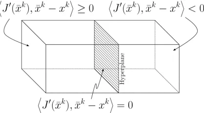
The final extragradient method that we implement is Hyperplane method

[16, 32] of the following form:

¯

xk=P_A(xk−αkJ0(xk)) xk+1=PA(xk−λkJ0(x¯k)) (3.22)

whereαk>0is located through a finite bracketing procedure and

λk=

hJ0(x¯k),x¯k−xki ||J0(x¯k_)||2 .

3.3. Extragradient Methods 28

Figure 3.1: Geometry of Hyperplane Extragradient Method

As it shows in the Figure 3.1, one side includes all the solutions of the

varia-tional problem. A hyperplane excludesxkthat satisfies the following condition:

hJ0(x¯k),x¯k−xki<0

It can be concluded that||xk+1−x∗|| ≤ ||xk−x∗||for any solutionx∗of the varia-tional problem. LetJ0be monotone and continuous, and the solution setA∗be

nonempty, then the hyperplane method converges [16].

Now, we can move forward to computational aspects of the extragradient

methods that we discussed above. We will state the step algorithms for each

method and implement for the following test problem:

Test Problem

a=1+x(x−1) +y(y−1) u=x(ex−e)y(ey−e)

(3.23)

We will solve the problem of finding the variable parameter in 2D elliptic BVP (1.1).

Here, we will formulate the regularized MOLS functional as a variational

3.3. Extragradient Methods 29

3.3.1

Khobotov’s Extragradient Method

In this section, we will state Marcotte’s variations to reduce step length. The

first one is known as the first modified version of Marcotte that keeps theαstay

bounded away from zero:

α =min

α 2, 1 √ 2

||xk−x¯k|| ||J0(xk_)−J0_(x¯k_)||

(3.24)

The second modified version of Marcotte that is stated in [32] changes the initial

α as following:

α =αk−1+

β ||x

k−1_−x¯k−1_||

||J0(xk−1_)−J0_(x¯k−1_)||−αk−1

γ (3.25)

whereγ ∈(0,1)and β ∈(0,1). This rule increases the α ifαk−1 is smaller than

optimal, and the reduction rule forα is the following:

α =max

ˆ

α,min

ε α,β ||x

k_−x¯k_||

||J0(xk_)−J0_(x¯k_)||

(3.26)

whereε∈(0,1). Therefore, these rules enable an adaptive alteration of the initial

value ofαk.

Here is the Khobotov algorithm with Marcotte’s two different choices to

re-duce step length:

Step 1: Choose initialx0∈A,β,α and setk=1

(a) Updateα =αk−1(Khobotov’s version for step length)

(b) Updateα =α_k−1+

β ||x

k_−x¯k_||

||J0(xk_)−J0_(x¯k_)||−αk−1

γ (Marcotte’s second

modi-fied version)

Step 2: ComputeJ0(xk)

Step 3: First Projection:x¯k=P_A(xk−αJ0(xk))and computeJ0(x¯k)

if J0(x¯k) =0 then x¯kis a solution of the problem.

else if α>β ||x

k_−x¯k_||

3.3. Extragradient Methods 30

(a) α=min

n α 2, 1 √ 2

||xk−x¯k|| ||J0(xk_)−J0_(x¯k_)||

o

(Marcotte’s first modified version)

(b) α=max

n

ˆ

α,min

n

ε α,β ||x

k_−x¯k_|| ||J0(xk_)−J0_(x¯k_)||

oo

(Marcotte’s second modified

ver-sion)

and go to Step 3.

else αk=α

Step 4: Second Projectionxk+1=P_A(xk−αJ0(x¯k))

Step 5: if||xk+1−xk||<T OL,STOP,elsek=k+1go to Step 2.

The Figure 3.2 shows the result of computing the variable parameter for given

2D elliptic boundary value problem (3.23).

3.3.2

Solodov-Tseng Method

Solodov and Tseng [28] propose a practical alternative to the extragradient method,

such that

¯

xk=PA(xk−αkJ0(xk)) xk+1=xk−γM−1(Tα(xk)−TαPA(x¯k)) (3.27)

whereγ is a positive step size, M is the scaling matrix that must be symmetric

and positive definite, and T_α = (I−αJ0); here I is the identity matrix. The

ex-tragradient method is modified by strongly monotoneTα andM−1. Moreover, it only requires one projection, and two function evaluations at each step.

More details about the method can be found in [28, 32]. The following is the

algorithm for the Scaled Extragradient Method that we use in our experiments:

Step 1: Choose initialx0∈A,θ ∈(0,2),ρ∈(0,1),α0>0and setk=1, positive,

sym-metric matrix,M.

3.3. Extragradient Methods 31

Figure 3.2: Solution by Second Modified Version of Marcotte

Step 3: if||rx||<T OLthen STOPelseα =α_k−1, f lag=0

Step 4: if J0(xk) =0thenxkis a solution of the problem.

Step 5: while

3.3. Extragradient Methods 32

ifflag6=0then updateα =αk−1β endif

updatex¯k=PA(xk−αJ0(xk))

computeJ0(x¯k)

flag=flag+1;

endwhile

Step 6: Updateαk=α

Step 7: Computeγ =θ ρ||xk−x¯k||2/||M−1/2(xk−x¯k−αkJ0(xk) +αkJ0(x¯k)||2

Step 8: Computexk+1=xk−γM−1(xk−x¯k−αkJ0(xk) +αkJ0(x¯k))

Step 9: rx=xk+1−xk k=k+1

go to Step 3.

endif

endif

The scaling matrixMcan be taken as the identity matrix for simplification. The

parameters θ,ρ,β has a vital role in the performance of the method. In our

experiments, we chose various parameters to find the best approximation. The

results can be found in the numerical experiments section.

Figure 3.3 shows the result of computing the variable parameter for given 2D

elliptic boundary value problem (3.23).

3.3.3

Improved Goldstein’s Method

Goldstein method was studied in [31] to solve variational inequality problems

by updating the step length iteratively, that is:

3.3. Extragradient Methods 33

Figure 3.3: Solution by Solodov-Tseng Method

whereβ_kis positive scaling parameter. Moreover, [31] proposed the He-Goldstein

Method which requires Lipschitz continuity and strong monotonicity of the

ob-jective function.

xk+1=xk− 1

βk

n

J0(xk)−PA[J0(xk)−βkxk]

o

3.3. Extragradient Methods 34

Furthermore, an improved version of the Goldstein’s method is provided in [31]

such that

xk+1 = x_k−γ αkr(xk,βk) (3.30)

r(xk,βk) = 1

βk

n

J0(xk)−P_A[J0(xk)−βkxk]

o

.

whereα =1−_4β1

kτ andγ ∈(0,2).

We are going to use (3.30) for our numerical experiments. The step algorithm

is the following:

Step 1: Choose initialx0∈A,ε >0,γ ∈(0,2),βU >βL >1/(4τ)whereβ0∈[βL,βU]

and setk=0.

Step 2: Compute

r(xk,β_k) = 1 βk

n

J0xk)−PA[J0(xk)−βkxk]

o

.

If||r(xk,βk)≤εthenxkis a solution to the problem.

Step 3: Compute the next iterationxk+1=x_k−γ αkr(xk,βk)

Step 4: Updateβ_k

if||J0(xk+1)−J0(xk)|| βk||xk+1−xk|| <

1

2 setβk+1=max{βL, 1 2}βk

else if||J0(xk+1)−J0(xk)|| βk||xk+1−xk|| >

3

2 setβk+1=min{βU, 6 5}βk

Step 5: Setk=k+1and go to step 2.

Figure 3.4 shows the result of computing the variable parameter for given 2D

3.3. Extragradient Methods 35

3.3. Extragradient Methods 36

3.3.4

Hyperplane Method

Iusem [16] introduced a geometric interpretation of the extragradient methods.

The idea behind this algorithm is to use a hyperplane to separate the solutions

of the variational problem to the one side. The projection method is described

in (3.22). Here, if we fix αk=λk=α, then we obtain a similar iteration to

Kor-pelevich’s extragradient method [23].

We will need to chooseε ∈(0,1),αˆ,andα˜ such that0<αˆ <α˜ at initial step.

The step algorithm is the following [16]:

Step 1: Choose initialx0∈A,ε ∈(0,1), ,0<αˆ <α˜

Step 2: ifP_A(xk−αkJ0(xk)) =xkthen stop

elseselect the step length

if ||J0(x¯k)−J0(xk)|| ≤ ||x¯

k_−xk_|| 2 ˜αk2||J0(xk)||

then x¯k=x˜k

else f ind αk∈(0,α˜k) such that

ε ||x¯

k_−xk_|| 2 ˜αk2||J0(xk)||

≤ ||J0(P_A(xk−αkJ0(xk)))−J0(xk)|| ≤

||x¯k−xk||

2 ˜αk2||J0(xk)||

endif

ifJ0(x¯k) =0 then x¯k∈A∗ stop

else compute the new iterate

xk+1=P_A

xk−hJ

0_(x¯k_,xk_−x¯k_i

||J0(x¯k_)||2 J

0_(x¯k₎

Step 3: Setk=k+1and go to step 2.

Figure 3.5 shows the result of computing the variable parameter for given 2D

3.3. Extragradient Methods 37

Chapter 4

Performance Analysis

In this section, we will give a brief explanation for the performance analysis of

each method. We will emphasize the importance of choosing step length and

how it affects the efficiency of the extragradient method. Moreover, each

algo-rithm has constant parameters that we have to declare at the initial step. These

parameters play a significant role for the implementation of the extragradient

methods. We will use MOLS functional for our test problem unless otherwise

stated.

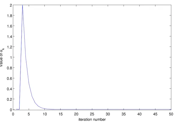
In the following Figure 4.1 and Figure 4.2, we show how the step length αk

alters depending on the extragradient methods, Solodov-Tseng and Improved

Goldstein’s method, respectively.

As we described in the previous chapter, Khobotov [18] uses a constant step

length for the extragradient method. However, the value of the parameter

af-fects how fast the algorithm converges. For example, if we setα =0.1, the

gra-dient norm decreases from0.0048to0.0047in nearly400iterations and in10000

iterations, the gradient norm becomes0.0030. On the other hand, forα =100,

39

Figure 4.1: Reduction Rule for Solodov-Tseng Method

Figure 4.2: Reduction Rule for Improved Improved Goldstein’s Method

The first modified version of the Marcotte rule cannot increase the value of

the step length whereas the second modified version of Marcotte can increase

40

α 0.1 100

L2-Error 0.0653 1.1890e-05

H1 error 1.1602 0.0779

2-norm 7.9882 0.1673

Table 4.1:α performance by Khobotov

Solodov and Tseng applies a reduction rule for step length by multiplyingαkby

a constantβ while the condition that is stated in the algorithm is satisfied.

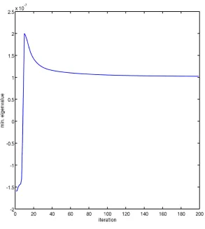
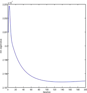
We solved the same test problem by using two different objective

function-als which are OLS and MOLS. We computed the minimum eigenvalues of the

hessian matrix at each iteration for both functionals. Figure 4.3 and Figure 4.4

illustrates the results for the first 200 iterations.

It is useful to state the minimum eigenvalue using MOLS functional is

pos-itive at each iteration which clarifies that MOLS is convex. On the other hand,

we obtain negative eigenvalues by using OLS function. We implement MOLS

functional on our test example since it is known that the MOLS is convex [12] .

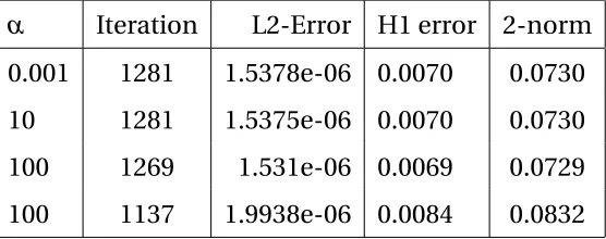
Table 4.2 gives the error analysis for various initial step length implementing

the second modified version of Marcotte method with MOLS functional.

α Iteration L2-Error H1 error 2-norm

0.001 1281 1.5378e-06 0.0070 0.0730

10 1281 1.5375e-06 0.0070 0.0730

100 1269 1.531e-06 0.0069 0.0729

100 1137 1.9938e-06 0.0084 0.0832

41

Figure 4.3: Performance Analysis of OLS

Table 4.3 gives the error analysis for various initial step length implementing

the second modified version of Marcotte method with OLS functional.

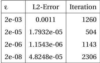
We already mentioned the importance of choosing regularization

parame-ter. Table 4.4 givesL₂ error analysis for different regularization parameters by using Marcotte (SMV).

To demonstrate, we can refer to Figure 4.5 that shows how the error gets

smaller when we get closer to the suitable regularization parameter. We can

also illustrate the definition of under-regularized and over-regularized solution

com-42

Figure 4.4: Performance Analysis of MOLS

α Iteration L2-Error H1 error 2-norm

0.001 771 4.2847e-04 0.1965 0.7200

10 771 4.2848e-04 0.1965 0.7200

100 772 4.2696e-04 0.1961 0.7186

100 558 3.6831e-04 0.1926 0.6486

43

ε L2-Error Iteration

2e-03 0.0011 1260

2e-05 1.7932e-05 504

2e-06 1.1543e-06 1143

2e-08 4.8248e-05 2306

Table 4.4: Regularization parameter,ε, performance

puted solution for differentε values. Whenε =2E−8, the solution is

under-regularized which states that we need to implement a bigger value for

regu-larization parameter. On the other hand, ε =2E−5gives an over-regularized

solution which clarifies that a smaller regularization parameter can give a

bet-ter result. Hence, ε =2E−6 gives the best approximation for Marcotte (SMV)

method.

We implement the extragradient methods for our test problem from the

pre-vious chapter. Here, we give the suitable regularization parameter for each method

and outputs forL₂−error, and H₁−error.

Extragradient Method Iteration ε L2-Error H1 error

Marcotte-SMV 1143 2e-06 1.1543e-06 0.0066

Solodov-Tseng 2150 8e-07 1.9382e-06 0.0077

Improved Goldstein’s 61907 8e-07 1.2149e-06 0.0031

Hyperplane 22511 2e-06 1.1399e-06 0.0066

Table 4.5: Performance analysis for the test problem

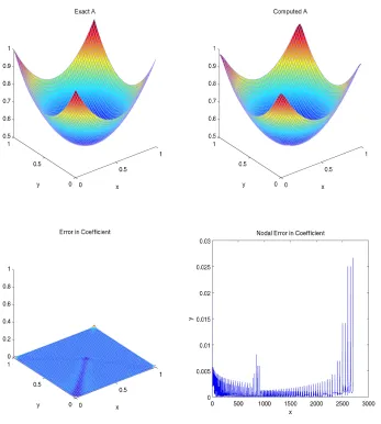
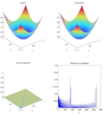
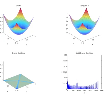
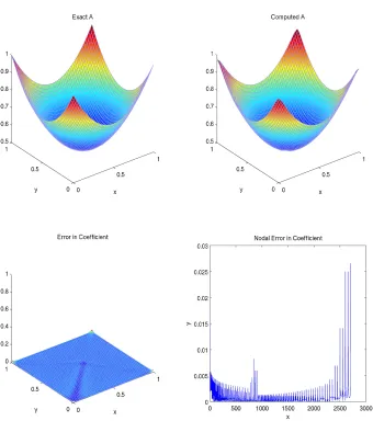
Computed solutions and errors by the extragradient methods can be found

in the previous chapter. Figure 4.6 demonstrates the computed solution by each

44

(a)ε=2E−8

(b)ε=2E−6 (c)ε=2E−5

45

test problem with n=50.

We can conclude that we get the best approximation by using Marcotte

meth-ods since these methmeth-ods have few parameters that we need to declare at initial

step. However, to choose the right step length at initial step still has a significant

role for the performance of the method. Solodov and Tseng introduces a scaled

matrix to accelerate the convergence. Moreover, Improved Goldstein’s method

is also very effective method. This method is also sensitive with the parameters

since choosing poor initial parameters may lead to over or under regularized

solutions.

Overall, changing only one parameter affects the entire algorithm and the

accuracy of the computed solution. Hence, we get better results with Marcotte

methods since it requires few parameters to be declared at initial step. That

is the reason why we mainly implemented Marcotte methods for performance

46

(a) Exact

(b) Marcotte (c) Solodov-Tseng

(d) Improved Goldstein’s (e) Hyperplane

Chapter 5

Background Material

Vector spaces and inner product play a significant role in understanding the

fi-nite element methods. Avector spaceis a set of vectors V on which two algebraic

operations are defined:

Vector addition:u,v∈V thenu+v∈V. It is clear to see that the vector addition is commutative and associative.

Scalar multiplication:u∈V andα ∈Rthenαu∈V.

It is important to note that functions can be written as vectors, thus they

satisfy the fundamental properties of vectors.

Definition 5.0.4(Vector Space). LetV be a vector space. (·,·)be an inner

prod-uct on V obtaining a real number by taking two vectors from V that holds the

following properties:

• (u,v) = (v,u)for allu,v∈V

• (αu+βv,w) =α(u,w) +β(v,w)for allu,v,w∈V and allα,β ∈R

• (u,u)≥0for allu∈V, and(u,u) =0if and only ifu=0.

48

Definition 5.0.5(Norm Space). LetV be a vector space|| · ||be a norm onV with

a real-valued function defined onV that holds the following properties:

• ||u|| ≥0for allu∈V, and||u||=0if and only ifu=0;

• ||αu||=|α|||u||for allu∈V and allα∈R

• ||u+v|| ≤ ||u||+||v||for allu,v∈V.

Therefore, we can define a norm onV as||u||=p(u,u)where(u,u)is an inner product onV.

Definition 5.0.6 (Banach Space). Let {X_n} be a Cauchy sequence in a normed

space X. If every Cauchy Sequence converges to a limit in X, then X is called

com-plete and every comcom-plete normed space is called a Banach space.

Theorem 5.0.7. Let V be an inner product space, then for allu,v∈V the following

properties hold:

1. |(x,y)| ≤ ||x|| ||y||

2. ||x+y|| ≤ ||x||+||y||

3. ||x+y||2_+||x−y||2_=2(||x||2_+||y||2₎

Definition 5.0.8(Linear Operators). Let X,Y be real vector spaces and define a

mapA:X →Y where

A(αu+βv) =αAu+βAv

holds for∀u,v∈D(A)andα,β ∈R, thenAis called a linear operator. Ais called

bounded if||Au|| ≤m||u|| ∀u∈X for a constantm>0.

LetA(u,v)be a symmetric bilinear form than the following properties will be

hold:

49

2. a(αu+βv,w) =αa(u,w) +βa(v,w) f or all u,v,w∈V and all α,β ∈R

3. a(u,u)≥0, andu=0then a(u,u) =0

Moreover, in some cases, the bilinear forma(·,·)can also hold the following properties:

4. There existsα>0such thata(u,u)≥α||u||2for allu∈V. (V-elliptic)

5. There existsβ >0such thata(u,v)≤β||u|| ||v||for allu,v∈V.(Bounded)

Definition 5.0.9 (Dual Space). X∗ is called dual space consisting of all linear

functionals on a normed space X that is defined by

||f||= sup x∈X,x6=0

|f(x)| ||x||

Definition 5.0.10 (Hilbert Spaces). Let H be a Hilbert space, the it satisfies the

followings

1. H is a vector space.

2. H is an inner product space that is(·,·):H×H →K(K is a scalar field) such that

i (u,v) = (v,u)

ii (αx+βy,z) =α(x,z) +β(y,z)

iii (x,γy+δz) =γ¯(x,y) +δ¯(x,z)

iv (u,u)≥0with equality holding if and onlyu=0

3. H is a normed space such that|| · ||=p(·,·)

4. H is complete.

50

Now, we can state two well-known inequalities, that are

1. Cauchy-Schwarz Inequality|(x,y)| ≤ ||x|| ||y||

2. Minkowski Inequality||x+y|| ≤ ||x||+||y||

Theorem 5.0.11(Riesz Theorem). Let H be a Hilbert space, then every f ∈H∗can

be represented by inner product, that is

f(x) = (x,y)

where||f||=||y||.

Theorem 5.0.12(The Lax-Milgram theorem). Let V be Hilbert space anda(u,v)

be V-elliptic, bounded bilinear form such that

|a(u,v)| ≤β||u|| ||v|| f or all u,v∈V,β >0

||a(v,v)|| ≥α||v||2v∈V,α >0

Let f ∈V∗, then there exist a unique solution u∈V to the variational problem such that

a(u,v) = f(v) f or all v∈V and the solutionucontinuously depends on f such that

||u||V ≤ 1

α||f||

∗ V

Definition 5.0.13. Define an operatorA:X→X∗on the real Banach spaceX.

Monotone: (Au−Av,u−v)≥0 f or all u,v∈V

Strongly Monotone: (Au−Av,u−v)≥c||u−v||xp f or all u,v∈X,where c>0and p>1

51

Convexity: A functional f :A⊂X →R is a convex set in the real normed space X that is: f((1−t)u+tv)≤(1−t)f(u) +t f(v) f or all t∈[0,1]u,v∈A

Lemma 5.0.14. LetHbe a real Hilbert space, and A be a nonempty, closed , convex

subset ofH. For eachx∈Hthere is a uniquey∈Asuch that

||x−y||=inf

z∈A||x−z|| (5.1)

whereyis called the projection ofxonAsuch that

y=PAx

Definition 5.0.15. Let Mbe a metric space and F :M→M is called contraction

mapping if

d(F(x),F(y))≤k dˆ (x,y), x,y∈M for some0<kˆ<1. Ifkˆ=1thenMis called nonexpansive.

Theorem 5.0.16. The projection ofxonA,y=P_AxwhereAis a closed convex set

of Hilbert space, if and only if:

y∈A:hy,z−yi ≥ hx,z−yifor all z∈A

Lemma 5.0.17. The projection operator satisfies the following properties [19]:

(a) ||P_Ax−P_Ay|| ≤ ||x−y||for all x,y∈H

(b) hx−P_Ax,P_Ax−yi ≥0 for all x∈H, y∈A

(c) ||x−y||2≥ ||x−P_Ax||2+||y−P_Ax||2 for all x∈H, y∈A

52

(a) (b) (c)

Bibliography

[1] R. Acar, Identification of the coefficient in elliptic equations,SIAM J.

Con-trol Optim., 31, (1993), 1221–1244.

[2] A. S. Antipin, B. A. Budak, F. P. Vasil´ev, A first-order continuous

extragradi-ent method with a variable metric for solving equilibrium programming

problems. (Russian) Vestnik Moskov. Univ. Ser. XV Vychisl. Mat. Kibernet.

2003, no. 1, 37–41, 56; translation in Moscow Univ. Comput. Math.

Cyber-net. 2003, no. 1, 43–47

[3] A. Bnouhachem, M. Aslam Noor, Z. Hao, Some new extragradient

itera-tive methods for variational inequalities. Nonlinear Anal. 70 (2009), no. 3,

1321–1329.

[4] A. Bnouhachem, Abdellah; X. Fu, M. H. Xu, and S. Zhaohan,Modified

ex-tragradient methods for solving variational inequalities. Comput. Math.

Appl. 57 (2009), 230–239.

[5] A. Bnouhachem, Abdellah; X. Fu, M. H. Xu, and S. Zhaohan, New

extragradient-type methods for solving variational inequalities. Appl.

BIBLIOGRAPHY 54

[6] Y. Censor, A. Gibali, S. Reich, The subgradient extragradient method for

solving variational inequalities in Hilbert space. J. Optim. Theory Appl.

148 (2011), no. 2, 318-335.

[7] Y. Censor, A. Gibali, S. Reich, Strong convergence of subgradient

extra-gradient methods for the variational inequality problem in Hilbert space.

Optim. Methods Softw. 26 (2011), 827–845.

[8] Y. Censor, A. Gibali, S. Reich, Extensions of Korpelevich’s extragradient

method for the variational inequality problem in Euclidean space.

Op-timization 61 (2012), 1119–1132.

[9] M. S. Gockenbach, Partial Differential Equations Analytical and

Numeri-cal Methods. SIAM, (2002).

[10] M. S. Gockenbach, Understanding and Implementing the Finite Element

Method. SIAM, (2006).

[11] M. S. Gockenbach, A. A. Khan, Identification of Lam´e parameters in linear

elasticity: a fixed point approach, J. Ind. Manag. Optim. 1 (2005)487–497.

[12] M. S. Gockenbach, A. A. Khan, An abstract framework for elliptic inverse

problems. Part 1: an output least-squares approach, Math. Mech. Solids,

12 (2007) 259–276.

[13] M. S. Gockenbach, B. Jadamba, A. A. Khan, Numerical estimation of

dis-continuous coefficients by the method of equation error, Int. J. Math.

Comput. Sci., 1 (2006) 343–359.

[14] M. S. Gockenbach, B. Jadamba, A. A. Khan, Equation error approach for

elliptic inverse problems with an application to the identification of Lam´e

parameters, Inverse Problems in Science and Engineering, 16 (2008) 349–