Evolution of coupled lives' dependency across generations and pricing impact

City, University of London Institutional Repository

Citation

:

Luciano, E., Spreeuw, J. and Vigna, E. (2012). Evolution of coupled lives'

dependency across generations and pricing impact (Actuarial Research Paper No. 199).

London, UK: Faculty of Actuarial Science & Insurance, City University London.

This is the unspecified version of the paper.

This version of the publication may differ from the final published

version.

Permanent repository link:

http://openaccess.city.ac.uk/2330/

Link to published version

:

Actuarial Research Paper No. 199

Copyright and reuse:

City Research Online aims to make research

outputs of City, University of London available to a wider audience.

Copyright and Moral Rights remain with the author(s) and/or copyright

holders. URLs from City Research Online may be freely distributed and

linked to.

Faculty of Actuarial

Science and Insurance

Actuarial Research Paper

No. 199

Evolution of coupled lives’ dependency

across generations and pricing impact

Elisa Luciano,

Jaap Spreeuw

& Elena Vigna

May 2012

Cass Business School

106 Bunhill Row

London EC1Y 8TZ

Tel +44 (0)20 7040 8470

Evolution of coupled lives’dependency across

generations and pricing impact

Elisa Luciano

Jaap Spreeuw

_{Elena Vigna}

_.

25th May 2012

Abstract

This paper studies the dependence between coupled lives - both within and across generations - and its e¤ects on prices of reversionary annuit-ies in the presence of longevity risk. Longevity risk is represented via a stochastic mortality intensity. Dependence is modelled through copula functions. We consider Archimedean single and multi-parameter copulas. We …nd that dependence decreases when passing from older generations to younger generations. Not only the level of dependence but also its fea-tures - as measured by the copula - change across generations: the best-…t Archimedean copula is not the same across generations. Moreover, for all the generations under exam the single-parameter copula is dominated by the two-parameter one. The independence assumption produces quanti-…able mispricing of reversionary annuities. The misspeci…cation of the copula produces di¤erent mispricing e¤ects on di¤erent generations. The research is conducted using a well-known dataset of double life contracts.

JEL classi…cation: C12, C18, G22, J12.

Keywords: copula, goodness-of-…t, signi…cance test, stochastic mortal-ity, generation e¤ect, reversionary annuity.

1

Introduction

Longevity risk, i.e. the risk that individuals live longer than expected, has become an issue. The ageing population in industrialized countries creates a natural link between …nancial and actuarial problems, i.e. annuity pricing for pension schemes. Due to ageing population, public and private pension systems will play a crucial role in …nancing the needs of most individuals. Both in the

Università di Torino, ICER and Collegio Carlo Alberto, Italy. Email: luciano at econ.unito.it

y_{Faculty of Actuarial Science, Cass Business School, City University London. Email:}

j.spreeuw at city.ac.uk

z_{Università di Torino, Collegio Carlo Alberto and CeRP, Italy. Email: elena.vigna at}

…rst and in the second pillar the o¤er of insurance products increasingly includes last survivor and reversionary annuities. Given these features, the problem of their correct and accurate pricing becomes more and more relevant. Assessing the correct dependency between two members of a couple is the …rst step in this direction. Investigating whether and how this dependency evolves over time, i.e. considering di¤erent generations, is a second important aim. The …rst issue has been addressed in the literature, at least to a certain extent. To the best of our knowledge, the second has not been tackled, since it requires a treatment of longevity risk too. We believe that knowledge of the nuances of dependence and its evolution through generations could help in the long-time horizon planning of a life o¢ ce. Therefore, we address both issues in this paper.

The existing actuarial literature rejects the independence assumption and measures both the level of dependence and the extent of mispricing through the comparison between premia of insurance products on two lives with and without independence. In this …eld, the seminal paper is Frees et al. (1996), which introduces a dataset of couples of individuals provided by a large Canadian insurer. Their paper has been followed by a few others, including Carriere (2000), Denuit et al. (2001), Youn and Shemyakin (2001), Shemyakin and Youn (2006), and Luciano et al. (2008). Some of these papers were written before longevity risk became an issue. Others already include stochastic mortality. Consciousness of longevity risk indeed arose at the individual level, leading to the adoption of stochastic mortality - or stochastic intensity - models, in which the actual mortality rate can be di¤erent from the forecasted one. When couples are considered, one has to model both marginal stochastic mortality - taking the due age and generation e¤ects into account - and dependence. The latter aim is achieved by coupling marginal longevity risks with a copula function. Youn and Shemyakin (2001) and Shemyakin and Youn (2006) address the existence of dependence between the members of a couple, without performing a best-…t copula analysis. Carriere (2000), Denuit et al. (2001) and Luciano et al. (2008) investigate which copula encapsulates dependence better, i.e. how dependence “looks like”.

The academic literature on the static features of dependence is therefore existing, even though young. Up to our knowledge studies on the evolution of dependency across generations do not exist yet.

The present paper aims at deepening the study of dependence between mem-bers of a couple in two directions. Firstly, by addressing its evolutions over time, i.e. across generations. Secondly, by extending the features of dependence ad-dressed and the copulas used, mainly from one parameter to multi-parameter ones. By so doing, we extend Luciano et al. (2008) from a statistical (or best-…t) point of view, and also in terms of pricing consequences.

divorces, the creation of enlarged families, the increased independence of women in the family and so on. Not only the level of dependence but also its features - as measured by the copula - change across generations. Indeed, the best-…t Archimedean copula for a single generation is not the same across generations. However, for all the generations considered, goodness-of-…t and signi…cance tests indicate that two-parameters copulas are signi…cantly more suitable to describe dependence than one-parameter copulas. Less can be said on the comparison between two- and three-parameters copulas: the tests do not give clear answers regarding the dominance of one model on the other. The analysis of prices of reversionary annuities con…rms that dependence matters on pricing, for the independence assumption produces a quanti…able over- and under-pricing. Mis-pricing is heavier for older generations than for younger ones. Surprisingly, we …nd that even when the copula approach is adopted, the misspeci…cation of the copula has di¤erent and opposite e¤ects on the mispricing for di¤erent generations.

The paper is organized as follows. In Section 2 we present the methodology. In Sections 3 and 4 we present respectively the calibration method - as required by the speci…c data-set - and its results. In Section 5 we discuss the e¤ect of di¤erent models on premia of reversionary annuities, comparing them with the independence assumption. Section 6 concludes.

2

Methodology

This paper models mortality of couples using a copula approach: the joint survival probability is written in terms of the marginal survival probabilities and a function - namely, the survival copula - which represents dependence. The calibration procedure is two-step, as usual in the copula …eld. The best …t parameters of the margins are chosen separately from the best-…t parameters of the copula. This section brie‡y describes the modelling and calibration choices in the two steps.

Let the lives of the generation selected be (x)and (y); belonging respect-ively to the genderm(males) and f (females). They have remaining lifetimes

Txm and Tyf, which are assumed to have continuous distributions. As usual in

actuarial notation, in the following(x)and (y)refer to the initial ages of male and female, respectively. Denote by Sm

x and Sfy the corresponding marginal

survival functions:

S_xm(t) = Pr [T_xm> t]; ₈t 0

S_yf(t) = Pr T_yf > t ; ₈t 0:

Denote asSxy(s; t)the joint survival function of the couple(x; y), i.e.

Sxy(s; t) = Pr Txm> s; Tyf> t 8s; t 0:

(s; t)₂[0;₁] [0;₁],S can be represented in terms ofSxm; Syf:

Sxy(s; t) =C(Smx(s); Syf(t)):

2.1

Marginal survival functions

For each generation we model the marginal survival functions of males and females with the stochastic-intensity or doubly-stochastic approach. This ap-proach is well established in the actuarial literature, see Dahl (2004), Bi¢ s (2005) and Schrager (2006). Within this approach, the random time of death

T of the individual is modelled as the …rst jump time of a doubly stochastic process, i.e. a counting process the intensity of which is itself a nonnegative, measurable stochastic process (s). Under some technical properties, this con-struction permits to write the marginal survival probabilities as

S_ij(t) = Pr(T_ij > t) =E exp

Z t

0

j

i(s)ds ; (1)

wherei=x; y; j=m; f.

As usual, we focus on the case in which the intensity is an a¢ ne di¤usion. This permits to write the marginal survival probability in (1) in terms of the intensity evaluated at time 0 and two functions of time, denoted as ( )and

( ). One can indeed show that

S_ij(t) = exp

h

j i(t) +

j i(t)

j i(0)

i

; (2)

where the functions j_i( )and j_i( )satisfy appropriate Riccati ODEs.

Previous papers motivate the appropriateness, among generation-based af-…ne intensities, of processes without mean reversion. Luciano and Vigna (2005, 2008), using the evidence provided by a comparison of competing models over the UK population, focused on the following intensity:

d j_i(s) =aj_i j_i(s)ds+ j_i

q

j i(s)dW

j

i(s); (3)

whereW_ij is a one-dimensional Wiener process, withaj_i( )>0and j_i 0. No-tice that the process (3), that belongs to the Feller family, is a natural stochastic extension of the Gompertz model.1 _{This is a desirable property, given that in}

general the Gompertz model is appropriate for ages greater than 35. In ad-dition, Carriere (2000) …nds that the Gompertz model outperforms competing mortality models on the same dataset used in this paper.

This is a parsimonious choice, involving only two parameters (aj_i; j_i) for each generationiand genderj. From the empirical point of view, it proved to …t a number of di¤erent datasets quite accurately. These are the reasons that

1_{In fact,} j

i(s)is an exponential force of mortality if j

motivate its adoption in this paper too. For such process we have

( j

i(t) = 0 j

i(t) =

1 exp(bjit) cj_i+dj_iexp(bj_it)

(4) where ₈ > > > < > > > :

bj_i =

r

aj_i 2+ 2 j_i 2

cj_i = b

j i+a

j i

2

dj_i =cj_i aj_i

and therefore2

S_ij(t) = exp

2

4 1 exp b

j it

cj_i +dj_iexp(bj_it)

j i(0)

3

5: (5)

2.2

Copulas

We follow a quite established tradition in survival modelling of couples, by restricting our attention to Archimedean copulas. We start from one-parameter copulas. Each of these copulas is obtained from a continuous, decreasing, convex function : [0;1]_![0;+₁]; the generator, such that (1) = 0. Using and its generalized inverse 1;the copula is de…ned as follows:

C(v; z) = 1 ( (v) + (z)): (6) One can indeed check that the resulting function has the right properties for being a copula. Usually the generator - and consequently the copula - contains one parameter, which we denote as . As in Luciano et al. (2008), we consider the following Archimedean copulas:

Name C(u; v)

Clayton u +v 1

1

Gumbel-Hougaard exp ( lnu) + ( lnv)

1

Frank 1_{ln 1 +}(e u 1)(e v 1)

e 1

Nelsen 4.2.20 ln exp u + exp v e

1

Special W+

p

4+W2 2

1

;withW =_u1 u +_v1 v

Table 1. Archimedean single-parameter copulas considered.

2_{The survival function given by (5) is biologically reasonable (i.e. it is decreasing over}

time) if and only if the following condition holds: ebjit j i

2

+ 2 dj_i 2 > j_i 2 2dj_icj_i:

While the …rst three copulae are common in the literature, the last two are not. They have been included because, di¤erently from the …rst three copulae, their association – as measured by the cross-ratio function – is increasing over time, which is what one would expect (see Spreeuw, 2006). In order to im-prove the …t of the copula, we then extend our exam to two-parameter families, obtained by combining the Archimedean copulas with the product copula. A combination which still produces a copula is the following:

C ; (u; v) =u1 v1 C (u ; v ) (7)

whereC is any Archimedean copula included in Table 1 and ₂[0;1]. Last, we extend our consideration to three-parameter families, built in a similar way:

C ; ; (u; v) =u1 v1 C (u ; v ) (8)

where ( ; ) ₂ [0;1] [0;1]. Both the Archimedean and the two–parameter Archimedean copulas of type (7) are symmetric, in the sense that

C (u; v) =C (v; u)

and

C ; (u; v) =C ; (v; u)

for any(u; v)₂[0;1] [0;1]:3

The three-parameter Archimedean copulas in (8) are not symmetric in the sense that

C ; ; (u; v)6=C ; ; (v; u);

Symmetry implies that conditional survival probabilities are equal across genders, while asymmetry allows for survivorship conditional on death of the spouse that are di¤erent when we condition on the male or on the female’s death. Indeed, the conditional probabilities that the male (female) dies aftert1(t2), given that

the female (male) dies att2(t1)are:

Pr(T_xm > t1jTyf=t2) =

@C(u; v)

@v _(u;v)=(Sm

x(t1);Syf(t2))

Pr(T_yf > t_2jT_xm=t₁) = @C(v; u)

@v _(v;u)=(Sm

x(t1);S

f y(t2))

;

de…ningt₁ andt₂ such thatSm

x(t1) =Syf(t2)andSfy(t2) =Sxm(t1).

These probabilities are not necessarily equal in reality. As an example one could consider the case wheret1 =t2. In the majority of cases, we would have

t₁< t₂, due to the higher mortality of males, compared to females. This is the

main reason why we include asymmetric copulas in the current study. Some people would argue that the …rst probability may be lower than the second due

3_{It can be proved (see e.g. Nelsen, 2006), that two random variables are exchangeable if}

to bereavement e¤ects which usually have a more severe impact on males than on females.

By testing whether a two-parameter family does capture dependence in a more signi…cant way than a single parameter copula, we are interested in ex-ploring the trade-o¤ between a less parsimonious model and its …t. By testing the three-parameter model, not only are we interested in pushing the trade-o¤ between parsimony and …t one step further, but we are also interested in capturing the symmetry or asymmetry between dependence of males on females and vice-versa. The three parameter model nests the two-parameter one,4 _when

= . Obviously, the last one nests all the Archimedean copulas, including the maximum, minimum and product, when = = 1, as well as the product copula alone, when = 0or = 0.

For the sake of simplicity, in the remainder of the paper we classify in di¤er-ent ways the copulas considered, according to their number of parameters. In particular, we have:

1. Class 1P: the class of one-parameter copulas included in Table 1;

2. Class 2P: the class of two-parameters copulas, extensions of copulas in Class 1P via (7);

3. Class 3P: the class of three-parameters copulas, extensions of copulas in Class 1P via (8).

3

Calibration methods

3.1

Marginal survival functions

We consider the large Canadian dataset introduced by Frees et al. (1996). In this dataset thousands of couples of individuals are observed in a timeframe of …ve years, from 29 December 1988 till 31 December 1993. In order to provide an estimate of the marginal parameters for each generation, (^aj_i;^j_i), we …rst identify the generations. The de…nition of generation strongly depends on the availability of data. Given the scarcity of data for each single year of birth of the dataset, and observing that persons with ages of birth close to each other can intuitively belong to the same generation, we de…ne a generation as the set of all individuals born in a fourteen-years time-interval, as in Luciano et al. (2008). We also keep the three-years age di¤erence between male and female of the same couple, as this is the average age-di¤erence between spouses in the whole dataset. We select two generations: 1900-1913, 1914-27 for males, 1903-1916, 1917-30 for females.5 _{From now on, we refer to these generations as “old” and}

4_{The asymmetric three-parameter model was introduced in the doctoral dissertation of}

Khoudraji (1995), under the supervision of Genest and Rivest. It is discussed in Genest et al. (1998). The latter paper also contains the proof that the three parameter function de…ned in (8) is a copula, and a way to simulate from it.

5_{To be more precise, the males of the older generation were born between 1.1.1900 and}

“young”. Notice that the members of each generation may enter the observation period in nineteen di¤erent years of age. For instance, the male members of the old generation may start to be observed at every age between 75 and 94. For notational convenience and according to Luciano et al. (2008), we will consider as initial age of each generation the smallest possible entry age, namely,x= 75

for the old male,x= 61 for the young male,y = 72for the old female, y= 58

for the young female.

Then, we extract from the raw data the Kaplan-Meier (KM) empirical dis-tribution for each generation and each gender.

The last step consists in using the KM data to calibrate the parameters of the intensity of each gender and generation, (^aj_i;^j_i). This is done by minimizing the squared error between empirical and theoretical probabilities, the former being the KMs, the latter being obtained by replacing the appropriate function

( )- i.e., (4) - in the survival function (5).

3.2

Copulas

The calibration of the copulas belonging to classes 1P, 2P and 3P proceeds through the pseudo-maximumlikelihood (PML) approach as in Genest et al. (1995), a brief outline of which will follow below. In order to use the meth-odology we need complete data. This is a relevant restriction for the dataset available. In fact, the …ve-years observation window of the dataset implies that the majority of couples under observation are censored data. Restricting our attention only to complete data makes the number of couples suitable for the investigation drop remarkably.

The restriction to complete data is unavoidable even in the absence of multi-parameter copulas, whenever the accent is on the evolution of dependence across generations. Indeed, suppose that the focus of the investigation is only on the comparison of dependence of di¤erent generations and the copulas considered are only one-parameter. Ideally it is possible to keep the vast number of censored data and perform the best-…t copula test within each generation with the Wang and Wells procedure, see Wang and Wells (2000), that is suitable for censored data.6 _{The Wang and Wells procedure involves selecting a starting point 2}

[0;1]in the calculation of the empirical Kendall’s taub. In turn, the selection of induces an overestimation ofb, on which the whole procedure is based, and the higher the higher the overestimation ofb. It can be shown that the value of strongly depends on the generation considered: the older the generation, the lower the cutting point and vice versa. Therefore, the overestimation of b strongly depends on the generation chosen, and is bigger with younger generations. This phenomenon is not acceptable if the focus of the paper is on the comparison of dependence among di¤erent generations. If the investigator wants to compare in a consistent way the association within a couple across di¤erent generations, she is bound to select smaller subsets of complete data.

This has disadvantages and advantages. On the …rst side, the price to pay in order to be able to make consistent comparisons across generations is a re-markable reduction of the size of the sample, which in our case becomesn= 66

for each generation. In spite of this, as Carriere (2000) notices, this approach is ine¢ cient due to the scarcity of couples, but informative. Indeed Carriere, when testing the null hypothesis of independence of the data, considered only the com-plete observations of the same data. As in Frees et al. (1996), he pooled all the generations together, rather than considering di¤erent generations. Also in his case the number of couples drops to a surprisingly low 229. On the second side, the advantage of working with complete data only is that it allows to employ relatively straightforward goodness-of-…t tests that appeared in the literature in recent years. We greatly bene…t of this possibility in performing signi…cance tests of goodness-of-…t of copulas with di¤erent numbers of parameters.

We now illustrate the PML approach. For survival copulas, the rank-based loglikelihood to be maximized with respect to the parameters has the form:

`( ) =

n

X

i=1

log

(

c 1 R

(1)

i

n+ 1;1

R(2)_i

n+ 1

!)

; (9)

where`( ) is the resulting log-likelihood with parameter (which can be real or vector valued); n is the number of data,c (u; v) = @2C_@u@v(u;v) is the density of the copula C and R(_ij) is the rank of part j of observation i; j _{2 f}1;2_g,

i _{2 f}1; ::; n_g. The motivation for using this pseudolikelihood and its intuitive

meaning are illustrated for instance in Cherubini et al. (2004).

3.3

Best …t copula among classes 1P, 2P and 3P

Once for each copula in each class (1P, 2P, 3P) the parameters have been selected using (9), we can …nd the best-…t copula among copulas with one, two and three parameters. In fact, there is no guarantee (and, indeed, it is not the case) that the best-…t copula remains the same in the three classes. Therefore we perform a best-…t-copula test among copulas belonging to the same class (in terms of number of parameters). This is done in a straightforward way, by comparing the loglikelihoods.

3.4

One vs multi-parameter copulas: signi…cance test

of parameters performs better than a full model with more parameters, within which it is nested. Both methods will be described brie‡y below.

3.4.1 AIC and BIC values

Let`( )be de…ned as in (9). Then, the Akaike Information Criterion (AIC) is de…ned as

AIC= 2

n(`( ) p);

wherepis de…ned as the number of parameters of c . On the other hand, the Bayesian Information Criterion (BIC) is de…ned as

BIC= 2

n `( )

logn

2 p :

In the vast majority of applicationsBICpenalizes more thanAICdoes, since

BIC > AIC for n > e2 _{7:39. Both criteria have also found their way in}

the actuarial literature. AIChas been applied by Frees and Valdez (1998) in comparing non-nested copula models …tted to a dataset consisting of losses and ALAE’s (Allocated Loss Adjustment Expenses), while Cairns et al. (2009) use

BICin judging on the performance of several mortality forecasting models. According to these methods, the lower theAIC (or BIC) value, the more suitable the model.

3.4.2 Statistical tests for nested models

When copula models are nested, it is possible to use the pseudolikelihood ratio test for nested models, introduced by Chen and Fan (2005). In this case, the following hypotheses have been tested:

1. (Model 1P versus Model 2P)H0: = 1

2. (Model 2P versus Model 3P)H0: = .

For instance, consider Hypothesis 1 with parameter estimates for Models 1P and 2P denoted by and b;b respectively. The test serves to reject the null hypothesis if twice the di¤erence between the loglikelihoods, that is

2

n

X

i=1

log

2 6 6 4

c 1 R

(1)

i n+1;1

R(2)i n+1

c_(b;b) 1 R

(1)

i n+1;1

R(2)i n+1

3 7 7 5;

4

Calibration results

4.1

Marginal survival functions

The parameters of the marginal survival functions, for both the OG (old gen-eration) and the YG (young gengen-eration) are presented (in basis points) in the following table:

OG male OG female YG Male YG Female

a 961.045 790.232 528.581 619.733 0.007 0.057 0.019 0.5

Table 2. Parameters of the marginal survival functions.

Their initial values for the two generations are x(0) = 0:036097and. y(0) =

0:016453:

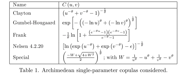
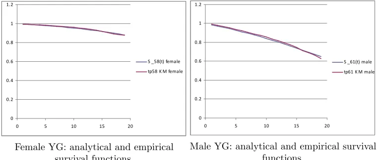
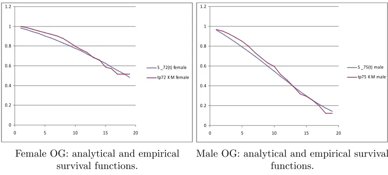
The following …gures report the plot of the survival probabilities, grouped by generation and gender. Each …gure reports the analytical survival function

Sz(t) for initial age z, and the empirical survival function obtained with the

Kaplan Meier methodology.

0 0.2 0.4 0.6 0.8 1 1.2

0 5 10 15 20

S _58(t) female tp58 K M female

Female YG: analytical and empirical survival functions.

0 0.2 0.4 0.6 0.8 1 1.2

0 5 10 15 20

S _61(t) male tp61 K M male

0 0.2 0.4 0.6 0.8 1 1.2

0 5 10 15 20

S _72(t) female tp72 K M female

Female OG: analytical and empirical survival functions.

0 0.2 0.4 0.6 0.8 1 1.2

0 5 10 15 20

S _75(t) male tp75 K M male

Male OG: analytical and empirical survival functions.

4.2

Joint calibration: decreasing dependence from OG to

YG

Following Genest and Rivest (1993), we …rst compute an estimate b of the Kendall’s tau coe¢ cient for each generation. The empirical estimateb for the Kendall’s tau is given by Table 3.

OG YG Kendall’s 0.440 0.279 Table 3. Kendall’s across generations.

Dependence decreases as we consider younger generations. Consistently with the decrease of the Kendall’s tau across generations, for each copula selected the dependence parameter is decreasing when passing from older to younger generations.

This interesting result is not surprising and is in accordance with the ob-served increase in the rate of divorces, the creation of enlarged families, the increased independence of women in the family and so on. We call this e¤ect “cohort e¤ect”.

“age e¤ect”. Because of the age e¤ect, one would expect a higher dependence coe¢ cient for the older generation evenwithout a cohort e¤ect.

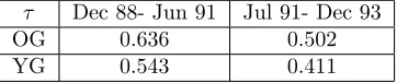
The dataset at hand does not allow us to separate the age and generation e¤ect. In order to do so, one would need either to observe the same cohort over two di¤erent time windows, i.e. at di¤erent ages, or di¤erent generations over di¤erent windows but when they have the same initial age. No one of these possibilities is open to us, since we have a unique time window. In order to cope with the problem, we proceed as follows:

We create arti…cially two observation windows out of the unique one, by distinguishing the period 29 December 1988–30 June 1991 from the period 1 July 1991–31 December 1993.

For each cohort we compute the Kendall’s tau in the two sub-windows, in which the same individuals have di¤erent initial ages.

Implementing this procedure we are observing the same generation with dif-ferent initial ages. We obtain the following results:

Dec 88- Jun 91 Jul 91- Dec 93 OG 0.636 0.502 YG 0.543 0.411

Table 4. Kendall’s across two close observations windows.

Table 4 shows the unexpected result that for each generation decreases when time passes, meaning that the dependence seems to decrease when the two members of the same cohort become older. This may be due to the small number of couples at disposal in the dataset, and to the fact that in order to implement the procedure we had to further reduce the number of couples in each sub-window. Had we found the opposite results (i.e. an increasing ) we would have been puzzled by the issue whether the decreasing Kendall’s tau of Table 3 was due to cohort e¤ects or to age e¤ects. The likely answer would have been “by both”, and it would have been impossible (with this dataset) to measure the extent of age e¤ect and cohort e¤ect. This would have remained an open issue.

However, the evidence produced by Table 4 indicates that – for the two generations under scrutiny –increasing age does not imply higher dependence. Transferring this conclusion to Table 3 (which is the best that we can do with this dataset), there seems to be no age e¤ect on the decreasing Kendall’s tau from OG to YG. In other words, in this dataset dependence decreases when passing from older to younger generations and this seems to be due only to cohort e¤ects and not also to age e¤ects.

we cannot perform. However, an insurance company endowed with a complete series of data on coupled lives would be able to perform this investigation and separate age from generation e¤ect on the Kendall’s tau. This would permit to further support our results that dependence is a¤ected by generations e¤ect and decreases when considering younger cohorts. A complete answer to this open issue would have important implications. In fact, we believe the changing dependency factor across di¤erent generations has an impact on the pricing of insurance policies on two lives that should not be overlooked.

4.3

Joint calibration: Archimedean copulas

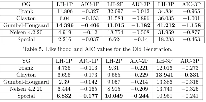
Following the method illustrated in Section 3, for each copula of Table 1 we calibrate the single-parameter and the two- and three-parameter versions. We then perform a best …t copula test among all copulas belonging to the same class in terms of number of parameters. The results are provided by the following two tables (the …rst one reports data for the old generation, the second one those for the young generation):7

OG LH-1P AIC-1P LH-2P AIC-2P LH-3P AIC-3P Frank 11:806 0:327 32:097 0:912 34:834 0:965

Clayton 6:04 0:153 31:583 0:896 36:035 1:001

Gumbel-Hougaard 14:396 0:406 41:015 1:182 41:212 1:158

Nelsen 4.2.20 4:919 0:12 18:754 0:508 31:959 0:877

Special 2:216 0:037 6:624 0:14 18:283 0:463

Table 5. Likelihood and AIC values for the Old Generation.

YG LH-1P AIC-1P LH-2P AIC-2P LH-3P AIC-3P Frank 4:736 0:113 9:31 0:221 12:016 0:273

Clayton 6:696 0:173 9:555 0:229 13:941 0:331

Gumbel-Hougaard 2:39 0:042 9:057 0:214 13:386 0:315

Nelsen 4.2.20 6:444 0:165 8:915 0:209 13:749 0:326

Special 6:832 0:177 10:049 0:244 10:951 0:241

Table 6. Likelihood and AIC values for the Young Generation. The results can be summarized as follows.

1. Class 1P: The one-parameter Archimedean family that performs best ac-cording to Tables 5 and 6 is the Gumbel-Hougaard for the old generation and the Special for the young generation.8

7_{In the tables, LH stays for loglikelihood. In the tables we report results only for AIC, the}

BIC values providing the same conclusions.

2. Class 2P: The two-parameters Archimedean family that performs best is the Gumbel-Hougaard for the old generation and the Special for the young generation.

3. Class 3P: The three-parameters Archimedean family that performs best is the Gumbel-Hougaard for the old generation and the Clayton for the young generation.

We see that for the old generation the winner copulas are nested, but they are not for the young generation. The following two tables report the value of the parameters for the winner copulas (the …rst one reports data for the old generation, the second one those for the young generation):

OG Gumb-Houg-1P Gumb-Houg-2P Gumb-Houg-3P

1:758 13:331 12:773 0:653 0:670

0:657

Table 7. Value of parameters for the best-…t copulas for the Old Generation. YG Special-1P Special-2P Clayton-3P

1:116 2:899 46:366 0:786 0:396

0:526

Table 8. Value of parameters for the best-…t copulas for the Young Generation. We then apply the signi…cance tests described in Section 3.4 to compare: (i) for the old generation: 1P-GH versus 2P-GH, then 2P-GH versus 3P-GH; (ii) for the young generation: 1P-Special versus 2P-Special, then 2P-Special

versus 3P-Clayton.

For the …rst three out of four comparison (nested models) we apply both AIC values and statistical tests, for the fourth comparison (non-nested models) we only use AIC values.

4.3.1 Signi…cance tests

For the Old Generation the p-values of the statistical test described in Section 3.4.2 are summarized in the following table:

OG 2P-vs-1P 3P-vs-2P P-value 0:001 0:019

From Table 9 we …nd that for the test 2P-vs-1P the Null Hypothesis (H0:

= 1) should be rejected at the signi…cance level of 5%, hence the two-parameters copula performs signi…cantly better than the single-parameter one. This is in accordance with the comparison between AIC values (and also BIC values, here not displayed), since AIC-2P<AIC-1P. Moreover, an additional investigation (the results of which are not displayed here) shows that the dom-inance of the 2P-copula on the corresponding nested 1P-one occurs for every copula of Table 1. This allows us to conclude that for the Old Generation of this dataset two-parameters copulas are signi…cantly more suitable to describe dependence than one-parameter ones.

Regarding the test 3P-vs-2P the Null Hypothesis (H0 : = ) should be

rejected at the signi…cance level of5%, hence the three-parameters copula per-forms signi…cantly better than the two-parameter one. However, this is not in accordance with the comparison between AIC values (and also BIC values, here not displayed), since this time AIC-2P<AIC-3P. So it is not clear which model is to be preferred.

As for the Young Generation, the test 2P-vs-1P gives a p-value of 0.0224, so on that basis we can reject the Null Hypothesis that 1P is a better model than 2P. Like the Old Generation, this is in accordance with the observation of the AIC (and BIC) values of both models.

Testing the Null Hypothesis that the 2P-model is signi…cantly better than the 3P-model is problematic. The Special and Clayton families are not nested, so it is not possible to conduct the aforementioned Chen and Fan tests. Chen and Fan (2005) also discuss a test for non-nested models, which however in this case leads to a high p-value (about 0.4, possibly due to the small dataset), and is therefore not informative. Relying just on AIC (and BIC) values would lead to the conclusion that the 3P-model (Clayton) is best for the given generation. Since for both generations the comparison 3P-vs-2P is either problematic or gives contradictory answers, and recalling that 2P copulas display symmetry while 3P ones do not, we have conducted a generic test on symmetry of bivariate copulas, due to Genest et al. (2012). Unlike the Chen and Fan test, this test does not requirea priorispeci…cation of the parametric copula, but is based on a consistent nonparametric estimate of the copula:

b

Cn(v; z) =

1

n

n

X

i=1

I_(Vb

i v;Zbi z);

whereVbi andZbi are such thatnVbi=R(1)i andnZbi=R(2)i . The null hypothesis

H0 simply states that the underlying copula is symmetric. The test statistic

centers on a distance between Cb(v; z) and Cb(z; v) of the Cramér-Von Mises type:

Sn =

1

Z

0 1

Z

0

n b

Cn(v; z) Cbn(z; v)

o2

dCbn(v; z);

(YG).9 So on this basis, we cannot reject the null hypothesis of symmetry at 5% signi…cance.

To sum up, for each generation two-parameters copulas are statistically signi-…cantly better than their one-parameter versions to describe dependence among the couples of this dataset. The comparison between two-parameters and three-parameters copulas does not provide clear answers. Whether the 3P-copula is dominant on the 2P-one depends on di¤erent factors, such as the generation and the criterion chosen.

5

E¤ects of dependence on pricing

In this section we present an actuarial application related to the pricing of policies on two lives. We consider areversionary annuity which pays1as long as both members are alive and a fractionRof it (Rstays for “reduction factor”) when only one member of the couple is alive. In this scheme, the last survivor product corresponds toR= 1and the joint life annuity corresponds toR= 0.

If the interest rate used in the actuarial evaluation is constant at the level

iover the maturity of the contract,10 _{the fair price of the reversionary annuity}

with reduction factorR₂[0;1]is

+1

X

t=1

vt R(tpmx tpxy) +R(tpfy tpxy) +tpxy ; (10)

wherev= (1 +i) 1 _{is the discount factor,(}

tpmx tpxy)is the probability that

the bene…tR is paid only to the male,(tpfy tpxy)is the probability that the

bene…tRis paid only to the female, andtpxy is the probability that the bene…t

1 is paid when both are alive. Connecting the survival probabilities needed to the marginal and the joint survival functions we have

tpmx tpxy=Sxm(t) Sxy(t; t); and tpfx tpxy=Syf(t) Sxy(t; t);

and also

tpxy=Sxy(t; t) =C(Sxm(t); Syf(t)):

Therefore, the price of the reversionary annuity is equal to

+1

X

t=1

vtR S_xm(t) +S_yf(t) 2C(S_xm(t); S_yf(t) + +

+1

X

t=1

vtC(Sm_x(t); Sf_y(t)):

9_{The function exchTest of the copula package "copula" in R (R Development Core Team,} 2011) was used to compute the results. For more details about the copula package in R, see Kojadinovic and Yan (2010).

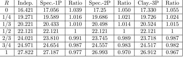
In practice, such contracts are quite common (see Frees et al., 1996) forR = 1=2;2=3. Therefore, we have implemented the pricing formulas when R takes the values0;1=4;1=3;1=2;2=3;3=4;1:Results are in the next section.

5.1

Prices of reversionary annuities

Tables 10 and 11 report the single premia ofR reversionary annuities for the Old Generation and the Young Generation, respectively. The interest rate used is i = 2%: While the …rst column reports the value of R, the second reports the price of the annuity under the independence assumption. For each model speci…cation (1P, 2P, 3P) there is a column reporting the best-…t copula price and another one reporting the ratio of the cum-dependence price to the inde-pendence one. In Table 10 “GH" stays for “Gumbel Hougaard", while in Table 11 “Spec." stays for “Special" and “Clay" stays for “Clayton".

R Indep. GH-1P Ratio GH-2P Ratio GH-3P Ratio

0 7:72 8:786 1:138 8:665 1:122 8:672 1:123 1=4 9:772 10:305 1:054 10:244 1:048 10:247 1:049 1=3 10:456 10:811 1:032 10:771 1:030 10:773 1:030 1=2 11:823 11:823 1 11:823 1 11:823 1 2=3 13:191 12:835 0:975 12:876 0:976 12:874 0:976 3=4 13:875 13:342 0:964 13:402 0:966 13:399 0:966 1 15:926 14:860 0:937 14:981 0:941 14:975 0:940

Table 10. Reversionary annuity price for OG under independence and using best-…t 1P–, 2P–, 3P–copulas.

R Indep. Spec.-1P Ratio Spec.-2P Ratio Clay.-3P Ratio

0 16:421 17:056 1:039 17:25 1:050 17:330 1:055 1=4 19:271 19:589 1:016 19:686 1:021 19:726 1:024 1=3 20:221 20:433 1:010 20:498 1:014 20:524 1:015 1=2 22:121 22:121 1 22:121 1 22:121 1 2=3 24:021 23:810 0:991 23:745 0:989 23:718 0:987 3=4 24:971 24:654 0:987 24:557 0:983 24:517 0:982 1 27:822 27:187 0:977 26:993 0:970 26:912 0:967

Table 11. Reversionary annuity price for YG under independence and using best-…t 1P–, 2P–, 3P–copulas.

The reader can notice the following.

2. For eachRand each model speci…cation (1P, 2P, 3P) the YG shows ratios of cum-dependence to independence price that are closer to1 than those of the OG. This is a clear consequence of the decreasing from OG to YG: the milder dependence of the YG generates prices that deviate less from the independence prices than the OG prices.

3. In both tables and for each model speci…cation (1P, 2P, 3P) each annuity has a value increasing in R, as expected, both under dependency and independency. This is obvious: a higher reduction factor implies a higher actuarial value of the bene…ts to be paid.

4. In both tables and for each model speci…cation (1P, 2P, 3P) the ratio cum-dependence/independence is decreasing whenR increases. This can be explained too. Let us recall that for R = 0 we have the joint life annuity (as nothing is paid to the last survivor) and for R= 1 we have the last survivor policy (where the bene…t paid remains constant also after the …rst death). Then,R measures the weight given to the last-survivor part of the reversionary annuity, with respect to the joint-life part. When

R = 0 positive dependence implies that the joint survival probability is higher than in the independence case, leading to a ratio greater than 1. At the opposite, whenR= 1we have the last survivor, for which positive dependence implies lower survivorship after the spouse’s death, implying ratios lower than 1. The values 0 < R < 1 give all the intermediate situations between these two extremes. In particular, for R₂(0;1=2)we still have ratios greater than1, forR₂(1=2;1)we have ratios lower than

1. For R= 1=2, the ratio is exactly1, in that the annuity price is shown to be una¤ected by the level of dependence. In fact, due to (10), the joint survival probability does not enter the premium that turns out to be:

+1

X

t=1

vt tp

m x +tpfy

2

! :

In this case, the weight given to the last survivor bene…t is equal to that given to the joint life annuity, and the two opposite e¤ects of overestima-tion and underestimaoverestima-tion of the premium perfectly o¤set each other. 5. The practical consequence of having ratios greater than 1 as long as

R <1=2and ratios smaller than1whenR >1=2is that insurance

measure of the extent of prudence so obtained. Consistently with item 2 above, prudence decreases when the younger generation is selected. 6. In both tables the prices and the ratios of 2P and 3P copulas are almost

identical. This is reassuring, given that the signi…cance tests displayed in Section 4.3.1 do not assess the dominance of either model on the other. For this reason, in the following items we will focus only on the 2P class and neglect the 3P class.

7. For the OG the impact on prices and on the ratio cum-dependence/independence is smaller for the 2P copulas than for the 1P copula; the opposite happens for the young generation. As a consequence, for the OG, the width of the range of prices and ratios when R changes is smaller for the 2P copulas than for the 1P copula; the opposite happens for the YG.

8. Misspeci…cation of the copula produces opposite mispricing e¤ects on the two generations. Indeed, given the assessed superiority of the 2P model with respect to the 1P one (see Section 4.3.1), a comparison of annuity prices implies that for the OG when the dependence is described with a 1P copula rather than with a 2P one, the insurer over-prices annuities with

R <1=2, and under-prices annuities withR >1=2. Opposite results apply

to the YG: when the dependence is described with a 1P copula rather than with a 2P one, the insurer under-prices annuities withR <1=2, and over-prices annuities withR >1=2.

Once more, not only dependence matters, but also its evolution across gen-erations - and the impact on pricing - matters and is not uniform.

6

Conclusions

This paper analyzes …rst from a statistical, then from a pricing point of view -dependence between coupled lives of insureds and its evolution. We model the margins of the two spouses with the doubly stochastic setup, and their depend-ence with the copula approach. Our main aim is to perfect the existing research in single generation dependence models, when longevity risk is accounted for. We develop the statistical analysis in two directions.

The …rst direction is to study the evolution of dependency across generations. We …nd that in the largest dataset on couples publicly available, dependence decreases when passing from older to younger generations. We …nd that this decrease in dependence is due to the cohort e¤ect only and not to the age e¤ect. We provide a methodology that, whenever su¢ ciently rich datasets were available, would allow to separate further age and cohort e¤ect on the evolution of dependence.

best copulas with signi…cance tests that penalize for the number of parameters. We …nd that two-parameters copulas are signi…cantly more suitable to describe dependence than single-parameter ones. This seems to be a new result in the literature on dependency among coupled lives. On the other hand, there are not enough elements to assess the dominance of the three-parameters class with respect to the two-parameters class, or vice versa.

After having performed statistical tests within and across generations, we study the e¤ect of dependence on pricing insurance products. Dependence does matter in pricing reversionary annuities, including joint-life and last-survivor ones. Indeed, when assuming independence the insurer under/over-prices rever-sionary annuities with a reduction factor lower/greater than a half. As for the comparison between generations, surprisingly we …nd that the misspeci…cation of dependence a¤ects in a di¤erent way each cohort. In fact, when the insurer misspeci…es the copula (taking one-parameter rather than two-parameters) the sign in the over- and underestimation is reversed depending on the generation under scrutiny and the reduction factor. This shows that mispricing caused by inaccurate modelling of dependence is not uniform across cohorts.

References

[1] Bi¢ s, E. (2005). A¢ ne processes for dynamic mortality and actuarial valu-ations. Insurance: Mathematics and Economics, 37, 443–468.

[2] Carriere, J.F. (2000). Bivariate survival models for coupled lives. Scand-inavian Actuarial Journal, 17-31.

[3] Cairns, A.J.G., Blake, D., Dowd, K., Coughlan, G.D., Epstein, D., Ong, A., and Balevich, I. (2009). A quantitative comparison of stochastic mortality models using data from England and Wales and the United States. North American Actuarial Journal 13 (1), 1-35.

[4] Chen, X. and Y. Fan (2005). Pseudo-likelihood ratio tests for semipara-metric multivariate copula selection. The Canadian Journal of Statistics 33 (3), 389-414.

[5] Cherubini, U., Luciano, E. and Vecchiato W. (2004). Copula methods for …nance, John Wiley and Sons.

[6] Dahl, M. (2004) Stochastic mortality in life insurance: market reserves and mortality-linked insurance contracts.Insurance: Mathematics and Eco-nomics 35, 113–136.

[7] Denuit, M., Dhaene, J., Le Bailly de Tilleghem, C. and Teghem, S. (2001). Measuring the impact of dependence among insured lifelengths. Belgian Actuarial Bulletin 1 (1), 18-39.

[9] Frees, E.W., and Valdez, E.A. (1998). Understanding relationships using copulas. North American Actuarial Journal 2 (1), 1-25.

[10] Genest, C and A.-C. Favre (2007). Everything you always wanted to know about copula modeling but were afraid to ask. Journal of Hydrologic En-gineering 12 (4), 347-368.

[11] Genest, C., Ghoudi, K. and L. Rivest (1995). A semiparametric estimation procedure of dependence parameters in multivariate families of distribu-tions.Biometrika 82 (3), 543-552.

[12] Genest, C., Ghoudi, K. and L. Rivest (1998). Commentary on "Under-standing relationships using copulas", by Freez, E.W. and Valdez, E.A., North American Actuarial Journal 2, 143-149.

[13] Genest, C., Nešlehová, J., and Quessy, J.-F. (2012). Tests of symmetry for bivariate copulas. Annals of the Institute of Statistical Mathematics, forthcoming.

[14] Genest, C., Quessy, J.F., and Rémillard, B. (2006). Goodness of …t proced-ures for copula models based on the probability integral transformation, Scandinavian Journal of Statistics, 1-30.

[15] Genest, C. and Rivest, L.P. (1993). Statistical inference procedures for bivariate Archimedean copulas. Journal of the American Statistical Asso-ciation 88, 1034-1043.

[16] Khoudraji, A. (1995).Contributions à I’étude des copules et à la modélisa-tion des valeurs extrêmes bivariées. Ph.D. thesis, Université Laval, Quebec, Canada.

[17] Kojadinovic, I. and Yan, J. (2010). Modeling distributions with continuous margins using the copula R package.Journal of Statistical Software 34 (9), 1-20.

[18] Luciano, E., Spreeuw, J. and Vigna, E. (2008). Modelling stochastic mor-tality for dependent lives,Insurance: Mathematics and Economics,43, 234-244.

[19] Luciano, E. and Vigna, E. (2005). Non mean reverting a¢ ne processes for stochastic mortality”, Carlo Alberto Notebook 30/2006. ICER Working Paper 1/05.

[20] Luciano, E. and Vigna, E. (2008). Mortality risk via a¢ ne stochastic in-tensities: calibration and empirical relevance, Belgian Actuarial Bulletin, 8 (1), 5-16.

[22] R Development Core Team (2011).R: A language and environment for stat-istical computing. R Foundation for Statistical Computing, Vienna, Aus-tria. ISBN 3-900051-07-0, URL http://www.R-project.org/.

[23] Schrager, D. F. (2006). A¢ ne stochastic mortality.Insurance: Mathematics and Economics 40, 81-97.

[24] Shemyakin, A., and Youn, H., (2006). Copula models of joint last survivor analysis, Applied Stochastic Models in Business and Industry 22, 211-224. [25] Spreeuw, J. (2006). Types of dependence and time-dependent association

between two lifetimes in single parameter copula models,Scandinavian Ac-tuarial Journal 5, 286-309.

[26] Wang, W. and Wells, M.T. (2000). Model selection and semiparametric inference for bivariate failure-time data.Journal of the American Statistical Association 95, 62-72.

FACULTY OF ACTUARIAL SCIENCE AND INSURANCE

Actuarial Research Papers since 2009

Report

Number

Date

Publication Title

Author

188. January 2009 The Market Potential for Privately Financed Long Term Care Products in the UK. ISBN 978-1-905752-19-5

Leslie Mayhew

189. June 2009 Whither Human Survival and Longevity or the Shape of things to Come. ISBN 978-1-905752-21-8

Leslie Mayhew David Smith

190 October 2009 ilc: A Collection of R Functions for Fitting a Class of Lee Carter Mortality Models using Iterative fitting Algorithms*

ISBN 978-1-905752-22-5

Zoltan Butt Steven Haberman

191. October 2009 Decomposition of Disease and Disability Life Expectancies in England, 1992-2004. ISBN 978-1-905752-23-2

Domenica Rasulo Leslie Mayhew Ben Rickayzen

192. October 2009 Exploration of a Novel Bootstrap Technique for Estimating the Distribution of Outstanding Claims Reserves in General Insurance. ISBN 978-1-905752-24-9

Robert Cowell

193. January 2010 Surplus Analysis for Variable Annuities with a GMDB Option. ISBN 978-1-905752-25-6

Steven Haberman Gabriella Piscopo

194. January 2010 UK State Pension Reform in a Public Choice Framework.

ISBN 978-1-905752-26-3

Philip Booth

195. June 2010 Stochastic processes induced by Dirichlet (B-) splines: modelling multivariate asset price dynamics.

ISBN 978-1-905752-28-7

Vladimir Kaishev

196. August 2010 AcomparativeStudyofParametricMortalityProjection Models. ISBN 978-1-905752-29-4

Zoltan Butt Steven Haberman

197. April 2012 Are the Dimensions of Private Information More Multiple than Expected? Information Asymmetries in the Market of Supplementary Private Health Insurance in England*

ISBN 978-1-905752-31-7

Martin Karlsson Florian Klohn Ben Rickayzen

198. May 2012 Re-thinking households – Using administrative data to count and classify households with some applications.

ISBN 978-1-905752-32-4

Gillian Harper Les Mayhew

199. May 2012 Evolution of coupled lives’ dependency across generations and pricing impact.

ISBN 978-1-905752-33-1

Elisa Luciano,

Statistical Research Papers

1. December 1995. Some Results on the Derivatives of Matrix Functions. ISBN 1

874 770 83 2 P. Sebastiani

2. March 1996 Coherent Criteria for Optimal Experimental Design.

ISBN 1 874 770 86 7

A.P. Dawid P. Sebastiani

3. March 1996 Maximum Entropy Sampling and Optimal Bayesian

Experimental Design. ISBN 1 874 770 87 5

P. Sebastiani H.P. Wynn

4. May 1996 A Note on D-optimal Designs for a Logistic Regression

Model. ISBN 1 874 770 92 1

P. Sebastiani R. Settimi

5. August 1996 First-order Optimal Designs for Non Linear Models.

ISBN 1 874 770 95 6

P. Sebastiani R. Settimi

6. September 1996 A Business Process Approach to Maintenance:

Measurement, Decision and Control. ISBN 1 874 770 96 4

Martin J. Newby

7. September 1996.

Moments and Generating Functions for the Absorption Distribution and its Negative Binomial Analogue.

ISBN 1 874 770 97 2

Martin J. Newby

8. November 1996. Mixture Reduction via Predictive Scores. ISBN 1 874 770 98 0 Robert G. Cowell.

9. March 1997. Robust Parameter Learning in Bayesian Networks with

Missing Data.ISBN 1 901615 00 6

P.Sebastiani M. Ramoni

10. March 1997. Guidelines for Corrective Replacement Based on Low

Stochastic Structure Assumptions. ISBN 1 901615 01 4.

M.J. Newby F.P.A. Coolen

11. March 1997 Approximations for the Absorption Distribution and its

Negative Binomial Analogue. ISBN 1 901615 02 2

Martin J. Newby

12. June 1997 The Use of Exogenous Knowledge to Learn Bayesian

Networks from Incomplete Databases. ISBN 1 901615 10 3

M. Ramoni P. Sebastiani

13. June 1997 Learning Bayesian Networks from Incomplete Databases.

ISBN 1 901615 11 1

M. Ramoni P.Sebastiani

14. June 1997 Risk Based Optimal Designs. ISBN 1 901615 13 8 P.Sebastiani

H.P. Wynn

15. June 1997. Sampling without Replacement in Junction Trees.

ISBN 1 901615 14 6

Robert G. Cowell

16. July 1997 Optimal Overhaul Intervals with Imperfect Inspection and

Repair. ISBN 1 901615 15 4

Richard A. Dagg Martin J. Newby

17. October 1997 Bayesian Experimental Design and Shannon Information.

ISBN 1 901615 17 0

P. Sebastiani. H.P. Wynn

18. November 1997. A Characterisation of Phase Type Distributions.

ISBN 1 901615 18 9

19. December 1997 A Comparison of Models for Probability of Detection (POD) Curves. ISBN 1 901615 21 9

Wolstenholme L.C

20. February 1999. Parameter Learning from Incomplete Data Using Maximum

Entropy I: Principles. ISBN 1 901615 37 5

Robert G. Cowell

21. November 1999 Parameter Learning from Incomplete Data Using Maximum

Entropy II: Application to Bayesian Networks. ISBN 1 901615 40 5

Robert G. Cowell

22. March 2001 FINEX : Forensic Identification by Network Expert Systems.

ISBN 1 901615 60X

Robert G.Cowell

23. March 2001. Wren Learning Bayesian Networks from Data, using

Conditional Independence Tests is Equivalant to a Scoring Metric ISBN 1 901615 61 8

Robert G Cowell

24. August 2004 Automatic, Computer Aided Geometric Design of

Free-Knot, Regression Splines. ISBN 1-901615-81-2

Vladimir K Kaishev, Dimitrina S.Dimitrova, Steven Haberman Richard J. Verrall

25. December 2004 Identification and Separation of DNA Mixtures Using Peak Area Information. ISBN 1-901615-82-0

R.G.Cowell S.L.Lauritzen J Mortera,

26. November 2005. The Quest for a Donor : Probability Based Methods Offer Help. ISBN 1-90161592-8

P.F.Mostad T. Egeland., R.G. Cowell V. Bosnes Ø. Braaten

27. February 2006 Identification and Separation of DNA Mixtures Using Peak Area Information. (Updated Version of Research Report Number 25). ISBN 1-901615-94-4

R.G.Cowell S.L.Lauritzen J Mortera,

28. October 2006 Geometrically Designed, Variable Knot Regression Splines : Asymptotics and Inference. ISBN 1-905752-02-4

Vladimir K Kaishev Dimitrina S.Dimitrova Steven Haberman Richard J. Verrall

29. October 2006 Geometrically Designed, Variable Knot Regression Splines : Variation Diminishing Optimality of Knots.

ISBN 1-905752-03-2

Vladimir K Kaishev Dimitrina S.Dimitrova Steven Haberman Richard J. Verrall

30. November 2008 Scheduling Reentrant Jobs on Parallel Machines with a

Remote Server. ISBN 978-1-905752-18-8

Konstantin Chakhlevitch Celia Glass

31. November 2009 Probabilistic Expert Systems for Handling Artifacts in Complex DNA Mixtures. ISBN 978-1-905752-27-0

R.G.Cowell S.L. lauritzen J. Mortera

32. April 2012 Detecting a Family Trio in a DNA Mixture.

ISBN 978-1-905752-30-0

Robert G. Cowell

Papers can be downloaded from

Faculty of Actuarial Science and

Insurance

Cass Business School

Copyright 2012 © Faculty of Actuarial Science and Insurance, Cass Business School

106 Bunhill Row, London EC1Y 8TZ.