A procedure for in situ wind load reconstruction from structural response only based on field testing data

Contents lists available atScienceDirect

Journal of Wind Engineering

and Industrial Aerodynamics

A procedure for in situ wind load reconstruction from structural response

only based on

fi

eld testing data

A. Kazemi Amiri

, C. Bucher

a_{Vienna Doctoral Programme on Water Resource Systems, Karlsplatz 13/222, A-1040 Vienna, Austria} b_{Center for Mechanics and Structural Dynamics, Karlsplatz 13/206, A-1040 Vienna, Austria}

A R T I C L E I N F O

Keywords:

Augmented impulse response matrix Inverse modal wind load identification Operational modal analysis

A B S T R A C T

Thefield application of a proposed procedure for the wind load identification is presented. The wind loads is inversely reconstructed from measured structural response in time domain, using an augmented impulse response matrix. The inherent noise amplification, arising from the ill-conditioning associated with the inverse problem, is resolved by means of Tikhonov regularization scheme in conjunction with two techniques for optimal regularization parameter estimation. To increase the accuracy along with the availability of the measured response only at a limited number of sensor locations, the problem is projected onto the modal coordinates. The structural modal parameters are obtained by an operational modal analysis technique. The case study of this paper is a 9.1 m (30 ft) tall guyed mast. Numerical simulation was implemented byfinite element modeling of the mast and a realistic two dimensional multivariatefluctuating wind speeds, to verify the experimental results by analogy. The results are provided in time and frequency domain. Comparison of the experimental results with the numerical simulation, where actual loads are available, confirm the capability of the proposed method. Based on the existing analogy, the reconstructed wind load in higher modes, derived from different regularization parameter estimation techniques, can also be validated.

1. Introduction

Inverse identification of dynamic loads is a common problem in differentfields of engineering such as in engine-induced vibrations of vehicle chassis (Hebruggen et al., 2002; Leclèrea et al., 2005), moving loads on the bridges (Zhu and Law, 2002; Lee, 2014; Law and Zhu, 2011) or in wind-induced vibration of the structures (Kazemi Amiri and Bucher, 2014; Chen and Lee, 2008). The load identification problem is generally an example of the inverse problems with applica-tion to structural dynamics and vibraapplica-tions. Dynamic load identification becomes more appealing in the cases, where the excitation factor can not be directly observed through measurements. This could be due to either the nature of excitement cause or the restrictions of man-made apparatus. The dynamic wind load, as a consequence of the wind pressure with the continuous distribution on the structural elements, is a good example in this regard. Engineers can obtain plenty of advantages, if good knowledge on dynamic loads are available. Those advantages can be outlined from the design phase (e.g. improvements in the loading guidelines of the standards) up to the post-analysis phase, as in structural performance improvement (Ziegler and Amiri, 2013) or health monitoring of the in-service structures.

The design codes of practice for wind loading provide useful instructions for engineers. The required codification data is mostly acquired by wind tunnel testing (Holmes, 2007; Simiu and Scanlan, 1978). However, laboratory assisted simulation of a complex phenom-enon in wind tunnel is bound to uncertainty due to the numerous restricting factors. Therefore, the information obtained by wind load identification from the field measurement data can be beneficial to verification of the wind tunnel test data. Moreover, in situ recon-structed wind load data can be also utilized for a more realistic reliability and risk assessment of the in-service structures. Note that, usually for this analysis purpose, the numerical simulation results are used (Bucher, 2009; Augusti et al., 1984).

Recently, wind load reconstruction from response measurements was investigated in a couple of studies. However, these studies are not significant in number, compared to those, generally conducted in dynamic load identification area. Hence, there is a tangible need for more research studies, particularly on the wind load related issues from different aspects. The studies on the wind load reconstruction may be categorized with respect to the way they treat the input identification problem. For example, it is suggested inLaw et al.to reconstruct the wind force as nodal loads, acting on the structures in the physical

http://dx.doi.org/10.1016/j.jweia.2017.04.009

Received 30 June 2016; Received in revised form 6 April 2017; Accepted 18 April 2017

⁎_{Corresponding author.}

E-mail address:[email protected](A. Kazemi Amiri).

Available online 28 April 2017

0167-6105/ © 2017 The Authors. Published by Elsevier Ltd. This is an open access article under the CC BY-NC-ND license (http://creativecommons.org/licenses/BY-NC-ND/4.0/).

the noise magnification due to assuming an identity covariance matrix of the external loads, but instead suggests to additionally apply low-passfilter on the measurement data to remove noise in relatively higher frequencies. In this situation a good knowledge on the noise properties is inevitable, in order to set the digitalfilter properties such that the main contents of the response data remain intact. InLourens et al. (2012)an augmented Kalmanfilter (AKF) was introduced, that embeds the input load in the state equation and estimates the system state and input load simultaneously, using L-curve technique for finding the appropriate force covariance matrix. However,the drawbacks of this method due to sensor location or stability issues demonstrates that still the Tikhonov type solution acquired by dynamic programing are more robust in practice. It is stated inAzam et al. (2015), that by an expert guess on the covariance of the input and through a proposed dual Kalman filter, the drift effect in the estimated input load via imple-menting the augmented Kalmanfilter can be avoided. The addition of dummy measurement to the AKF scheme was another remedy for resolving the instability of thefilter, that is discussed inNaets et al. (2015). All of the latter studies, despite their novelties and capabilities, require some essential a priori information either on the measurement noise or on the applied load features mainly in terms of process covariance matrices. In case of wind load, the incompleteness of response data demands to apply a sort of order reduction to the system equations of motion. In this situation, a priori knowledge about the input becomes more critical, because the features of the projected input on the order reduction vector must exist. However, one should mention the computational efficiency of those methods as a notable strength, in comparison with the deconvolution methods.

With respect to the above-mentioned points, in this contribution an approach for wind load identification is adopted, when the following conditions hold: a) additional data or information on the wind characteristics of the site of the structure, acting wind load or noise nature is unavailable, b) structural response just on a limited number of points can be measured, c) the noise effect within solving the inverse problem should be resolved, d) only structural modal characteristics (natural frequencies, mode shapes and damping ratios) through a system identification method and accordingly modal analysis are available. The implementation of such method is principally simpler than the above methods, though at a cost of more computational effort. However this method can provide the a priori knowledge or cross-check possibility for the above methods, particularly in case of wind loading, where the wind loading properties are highly variable with respect to the wind speed change.

For a structure undergoing wind vibration, application of this procedure requires only the response data derived from the field measurement. The impulse response matrix, necessary to construct the input-output (dynamic load-response) relation, is generated based on a previous work of the authors (Kazemi Amiri and Bucher, 2015). The case study structure in this study is a 9.1 m (30 ft) tall guyed mast with tubular elements. The characteristics of the reconstructed modal wind loads have been inspected in time and frequency domain. As a matter of fact it is not feasible to measure the actual wind load in the field testing tasks. Consequently, in order to verify the experimental results, the numerical simulation of the same problem was implemen-ted. This is done by thefinite element model of the mast structure and

Those equations are decoupled into a set of one degree of freedom systems in modal coordinatesq, using the substitutionsu( ) =t Φq( )t and then premultiplying byΦT(Ziegler, 1998; Chopra, 1995):

t

mu¨ + ˙ +cu ku= ( )p (1a)

diag ζ ω diag ω t

q¨ + 2 [i i] ˙ +q [ i] =q P( ) 2

(1b) whereP=Φ pT andζi,ωidenote the damping ratio and natural circular

frequency atithmode, respectively. Note that, the overdots refer to the time derivatives. The steps of the proposed procedure for wind load reconstruction are as follows:

1. Thefirst step is identification of the structural modal parameters, i.e. ωi,Φrandζi. Hereafter, the subscriptrrefers to the reduced set of

identified mode shapes or measured response vectors, since these are just available at the sensor locations.

2. The measured response acquired from different sensor channels mounted on the structure is decomposed by means of the following equation:

t t

q( ) =Φ u( ) ∼

r r

†

(2) in whichΦ = [Φ Φr ] Φ

T

r r

T

† −1 _andq∼_{( )t denote the pseudo inverse of the} incomplete mode shapes matrix and the approximated modal response matrix, respectively.

3. The validity of the decomposed modal response is checked by means of its power spectrum or simply its Fourier transform; such that each modal response must only have one dominant vibration frequency corresponding to the natural frequency of the system at that mode. To this end, the contribution of all modes within the existing frequency range must be decomposed.

4. The modal impulse response matrices (IRM) of the system[hdi]are generated for each mode, according to the associated modal para-meters (Kazemi Amiri and Bucher, 2015).

The IRM together with the decomposed modal response from step 2 are utilized to set up the input-output relation for the inverse identification of the acting modal wind load, i.ePi, in the equation below:

q h P

{ } = [_i di]{ }i (3)

The elements of the modal displacement IRM[h_d] ∈ l l*

i  , wherel equals the total number of time steps, are derived based on the impulse response function at each mode (Kazemi Amiri and Bucher, 2015).

5. The following optimization problem, referred to as Tikhonov reg-ularization scheme, is solved for estimating the applied wind loadP∼i.

Tikhonov and Arsenin (1997):

⎧ ⎨ ⎩ ⎫ ⎬ ⎭ λ

q h P P

min ∼_i− i∼i + i ∼i

2 ₂ 2

Prior to solving the preceding optimization problem, the so-called optimal regularization parameterλishould be determined. To the

knowledge of the authors, there are two techniques that can estimate the regularization parameter without a priori knowledge on the measurement noise. Those techniques are L-curve (Hansen and O'Lary, 1993; Hansen, 2007) and generalized cross validation (GCV) (Wahba et al., 1979). L-curve is the log-log plot of the smoothened solution (identified load) versus the residual norm (difference between retrieved and actual response), corresponding to different values of regularization parameter, and the balancing regularization parameter lies in the corner of L-curve. GCV provides the following mathematical expression, whose minimizer is an estimate of the regularization parameter:

⎛ ⎝ ⎜⎜ ⎞ ⎠ ⎟⎟ ⎡ ⎣ ⎢ ⎢ ⎛ ⎝ ⎜⎜ ⎞ ⎠ ⎟⎟⎤ ⎦ ⎥ ⎥

∑

∑

V λ z n λ

s n λ n

n λ s n λ ( ) = + / 1 + i ν n λ i

ν i ν

n i ν i =1 2 2 2 =1 2 2 (5) wherez= [ , …,z1 zn] =U q∼i. The vectorUand scalarssνare the left-singular vectors and left-singular values corresponding to left-singular value decomposition of the modal IRM, i.e.[h_di].

6. If required, the identified modal wind load can be transferred to the modal subspace of another structure for the post analyses. This is the case when the performance of the existing structure under wind excitation, called here the primary structure, is supposed to be improved. To do this, the post analysis on the modified version of the structure, referred to as the secondary structure, should be carried out. Importance is attached to the point that transferring the identified load makes sense, if and only if the actual wind loadp, in the physical subspace, is the same for either structure. This condition requires both structure to have similar geometries with regard to their wind exposed areas. If such condition holds, then a transfer matrixTis sought, so that the modal subspaces between

two structures can be exchanged, with respect to the fact that

PSt =Φ pSt T i i .

T P∼St₁=∼PSt₂ ⇒ T ΦSt₁=ΦSt₂ (6)

In the above equationP∼St₁andP

∼

St₂denote the estimated wind loads in the modal subspace of the primary and secondary structure, respec-tively. Note that the latter is unknown. Multiplying bym ΦSt₁ St₁from the right-hand side, by virtue of modal mass orthogonality

Φ m ΦSt =I

T St St

1 1 1 , gives:

T=Φ m ΦSt T

St St

2 1 1 (7)

Usually the mass matrix of the primary structure is not available. Moreover, through the application of an OMA merely the modal parameters are identified and the mode shapes are not mass-normalized. On the other hand, the secondary structure mass matrix should exist, because for further analysis the mathematical model of the secondary structure is required. In this situation, the above transfer matrix can be derived in terms of the mass matrix of the secondary structure. Therefore, the same scheme as above is followed such that:

P =T P′

∼ ∼

St₁ St₂ (8a)

T′ =Φ mSt Φ

T St St

1 2 2 (8b)

The comparison of the latter with the Eq.(6)yields thatT can be determined indirectly by taking the inverse ofT′, namelyT=T′−1.

over time (e.g. seeSalcher et al. (2016)), the entire procedure has to be repeated.

3. Results

3.1. The structure and measurement setup

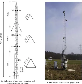
The structure is a 9.1 m (30 ft) tall guyed mast and consists of three parts. Each part of the mast has an equilateral triangular cross section, whose dimensions respectively from bottom to top are 0.43, 0.34 and 0.26 m (seeFig. 1a). Each part of the mast is composed of three main legs together with the horizontal and cross bracing elements, made of aluminium alloy. In order to prevent the excessive lateral displacement, three cables from either side account for the additional constraint on the upper part of the mast. The structure is located in Petzenkirchen, Austria and serves as a weather station tower in the Hydrological Open Air Laboratory (HOAL) (Blöschl et al., 2016).Fig. 1b shows an in situ picture of the mast structure.

The wind-induced acceleration response of the structures is mea-sured in horizontal plane of the mast via capacitive accelerometers, which are suitable for relatively low frequency vibration measurements. An almost evenly distributed configuration for the sensor locations was selected (see[ 1: 7]S S inFig. 1a). Such distributed configuration assists

to identify the mode shapes in all three parts, uniformly. Due to the poor vibration intensity around the guys connection, attachment of the sensors very close to those points was avoided. The vibration response was measured in two perpendicular direction (i.e.xandy) at locations S1, S3, S5, S6 and S7. The additional measurement in direction–yat the sensor locations S2 and S4 delivers the geometrical requirement for taking the coupled bending-torsional modes into account. As a result, there are 12 sensor channels in total. Through this sensor configuration one can measure general motion of the structure for a proper system identification. A representation of the measurement setup on the mast is shown inFig. 2.

3.2. OMA results

The modal characteristics of the structure have been identified based on the stochastic subspace identification method (Reynders and Roeck, 2008), by means of the so-called“MACEC”(Reynders et al., 2014). The sampling rate for data acquisition was set to 100 Hz. In order to have an insight into the eigenfrequencies of the system,firstly the acceleration power spectrum of different measured channels were observed. As an example, the power spectrum of the sixth channel at S4 (in direction-y) is illustrated inFig. 3a. For a better resolution, in the wind-induced vibration frequency range of interest, the signals were decimated by factor 7, which consequently yields to the new measur-able upper bound of 7.1 Hz with respect to the Nyqvist frequency. The power spectrum of the decimated signal is depicted inFig. 3b. Note that, all of thefirst four peaks are not clearly visible in thisfigure, as the signal belongs to only one direction. The signal processing including signal decimation and the offset removal should be also carried out before system identification.

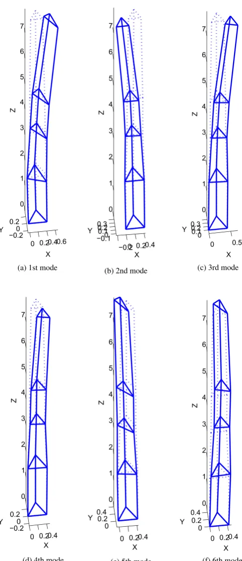
The results of OMA, regarding thefirst six identified modes, are Fig. 2.View of response sensors on mast and measurement arrangement.

Fig. 3.The measured signal power spectrum at sensor location S4.

Table 1

The identified natural frequencies and damping ratios of the mast structure.

Mode 1 2 3 4 5 6

Eigenfrequency (Hz) 3.03 3.31 3.44 3.53 5.49 6.58

provided inTable 1andFig. 4. Note that, in reality the identified mode shapes from experimental vibration data are complex-valued vectors (Mitchell, 1990; Caughey and O'Klley, 1965). As such, the identified mode shapes were realized via the complex transformation matrix (Niedbal, 1984; Friswell and Mottershead, 1995).

3.3. Identification of the wind load

In this study, solving the ill-posed inverse problem corresponding

to Eq.(3)forfluctuating part of modal wind loads was accomplished by Tikhonov regularization scheme (Tikhonov and Arsenin, 1997). The optimal regularization parameter, required for solving Eq.(4)has been determined by L-curve and generalized cross validation (GCV) techni-ques. Different methods are available that deal with the ill-posed inverse problems (e.g.see Hansen (1987), Klimer and O'Lary (2001) and Varah and Numer (1973)).

The accuracy of the regularized solution is inversely proportional to the size of the problem, i.e. the dimensions of matrices in Eq.(3). This in turn depends on the time length and the number of system degrees of freedom (dofs). The augmented IRM, introduced inKazemi Amiri and Bucher (2015), was used to set up the Eq.(3). The augmented IRM considers a linear evolution of the input between two consecutive time steps, namely implements thefirst order hold-type approximation. As such, the augmented IRM allows for larger time intervals for time discretization of the problem, in comparison with the ordinary IRM that assumes the step-wise constant input evolution. By projecting the physical coordinates onto the modal subspace two advantages are achieved. Firstly the multiple dofs system reduces to a number of single dof systems that gives rise to reduction of the problem size. Note that, generally the single parameter Tikhonov regularization treats the single unknown inverse problem much better than the case with multiple unknowns. This is due to the fact that there might be different degrees of ill-conditioning with respect to each unknown, while single regular-ization scheme cannot treat them individually but rather on average. There are methods developed based on the idea of multiple regulariza-tion levels like L-hypersurface (Belge et al., ) and multiple GCV (Modarresi, 2007). Those methods are considerably more complex in implementation than their single level regularization counterparts and are usually more efficient for the problems with a small number of unknowns. This condition does not hold for the case of wind loading that is present on a large number of dofs. The second advantage of modal projection is that, the continuous quantity of wind pressure/load acting on the structural element is discretized in modal subspace as an equivalent single force. As a result of the latter, the underdetermined state of the corresponding inverse problem, with respect to a limited number of sensor locations, is also resolved.

Afterwards, the type of the response quantity should be selected for the wind load reconstruction. Importance is attached to the point that the response type is another influential factor on the accuracy of recovered load. It is shown inKazemi Amiri and Bucher (2015)that the displacement is more suitable over the acceleration response, in order to infer the wind load from measured response.

3.3.1. Field application of the wind load identification

The case study structure is relatively a light-weight structure, therefore the accelerometers units were used in order to avoid the drastic effect of sensor mass on the behaviour of the structure. Consequently, the acceleration signal is integrated twice in frequency domain according to integral property of Fourier transform to obtain the displacement response (Brandt and Brincker, 2014). To prevent the drift phenomenon, which usually occurs because of signal integration, the signal is windowed and also passed through high-pass Butterworth filter with cut-in frequency of 0.2 Hz, every time before and after integration.

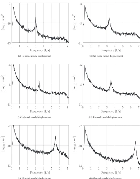
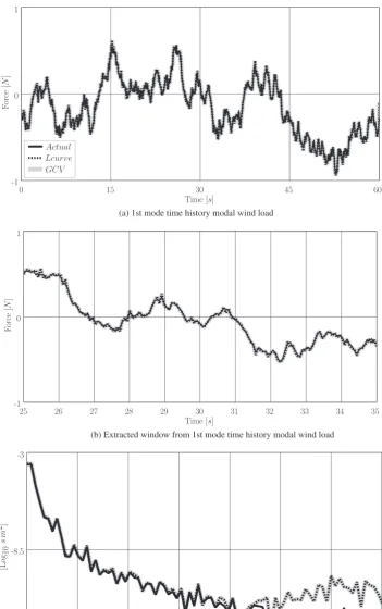
The displacement signals were decomposed into their modal response by means of the identified mode shapes, according to Eq. (2). In order to check the validity of the decomposed modal displace-ments response, the power spectrum pertaining to thefirst six modes are plotted inFig. 5. According to thisfigure, each signal features one dominant peak in the power spectrum corresponding to the modal natural frequency. This confirms that, the displacement response was correctly decomposed in the modal coordinates.

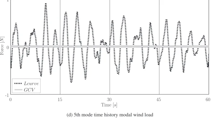
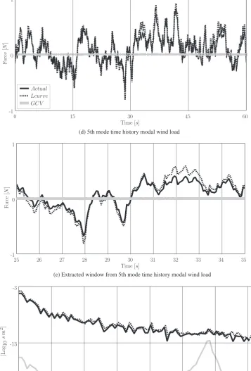
0.07 Sec associated with the sampling rate of the decimated signal (14.3 1/Sec). The identification results illustrate that the reconstructed modal loads by L-curve and GCV are almost identical in time history plots for thefirst four modes. On the other hand in thefifth and sixth modes, GCV (unlike L-curve) recovers the modal wind load only in the

4. Verification offield application results

In contrast to the numerical simulation, the applied wind load can not be directly measured in the experiments. Therefore, a procedure

was sought for verifying the identified modal wind loads indirectly. Some studies compare the retrieved response from identified wind load with the actual measured response. However, Eq.(3)is derived based on the convolution integral, and the IRM has a smoothing effect on the

applied load. It means that, for a highly or slightlyfluctuating identified load, apart from its validity, almost identical response might be retrieved (Hansen, 2007; Groetsch, 1984). As such, the results of the

domain between the features of the in situ and simulation-based reconstructed modal wind loads.

4.1. Simulation of the wind load reconstruction

The detailedfinite element of the mast structure was established in SlangTNG (Bucher and Wolff, 2013). The acting wind load along the structure is generated by the digital simulation of thefluctuating part of wind speeds in two perpendicular directions of the horizontal plane of the mast, independently at different height levels. The correlated fluctuating wind speeds were simulated at 18 height levels correspond-ing to the panels of the mast, with the assumption that wind speed is constant over one panel (seeFig. 1a). Then, the resulted wind forces due to the action of the wind pressure on the exposed area of the mast elements were considered as nodal loads, acting on the intersections of the mast elements.

The simulated noise-polluted response was achieved from the actual response, by adding the normalized white noise with adjustable noise level. The noise level was scaled with respect to the response standard deviation of the corresponding degree of freedom. The configuration of the virtual sensors as well as the measurement sampling rate are identical to that of thefield experiment. The reader is referred toKazemi Amiri and Bucher (2016)for more details on the problem simulation.

The time history and the power spectrum of the reconstructed wind load for the first mode with the eigenfrequency equal to 3.03 Hz is illustrated in Fig. 7. The results obtained by L-curve and GCV are almost the same and of a high accuracy. The corresponding result of thefifth mode with the eigenfrequency of 5.69 Hz is also represented in Fig. 7. Although GCV fails tofind the optimal solution at this mode, but L-curve provides a good quality recovered wind load signal. The noise level for the numerical simulation was set to 10% of the response standard deviations of the response at the virtual sensors locations.

According to the power spectrum plot inFig. 7c, it can be observed that a slight deviation of the identified signal power spectrum from that of the actual signal occurs only after the natural frequency of that mode. Consequently, the background signal is correctly identified. This leads to a negligible discrepancy between the identified and actual modal wind load signal in the time history plots. Analogous to the simulation results, the experimentally identified loads by GCV and L-curve are almost identical in time history with deviation of power spectrums after the natural modal frequencies. However, less discre-pancy is expected for the reconstructed loads by GCV, since the deviation in the spectrum of the GCV-based identified loads (after corresponding natural frequencies) are less compared to those recov-ered by L-curve.

The next interesting analogy exists between the results offifth and sixth modes. In simulation, GCV has obviously failed to recover the applied modal wind load except around related mode natural frequency similar to thefifth and sixth modes in thefield experiments (c.f.Fig. 6f and 7f). Nevertheless, L-curve could identify the wind load but relatively inaccurate compared to what for the first to fourth modes. As a result the validity of experimental results of thefifth and sixth modes can be verified, with a degree of uncertainty. Nevertheless the higher the mode number, the less contribution it has in the response to the input excitation, that reduces the effects of the inaccuracy in the identified modal load.

5. Conclusion

This contribution presented the field application of a proposed procedure for modal wind load identification inversely from full-scale measurement data of structural response. The major focus was drawn to the technical aspects of the practical application, including the case study, measurement setup, data processing and the utilized methods within the load identification procedure. It is important to note that all

information needed for wind load identification was obtained solely from the measurement data. In this regard, no additional information was required, either on the structural properties (e.g., any need to system mass, stiffness and damping matrices), or knowledge about the wind characteristics of the site of the structure.

The advantages of wind load reconstruction in the modal subspace, the use of displacement response and utilizing the augmented modal impulse response matrices was discussed profoundly. The modal parameters (natural mode shapes, natural frequencies and damping ratios) were required for the generation of the modal impulse matrices as well as decomposition of the measured displacement response. The structural modal properties were obtained by means of an OMA technique from the same ambient vibration testing data, which was then used for inverse load identification. The Tikhonov solution was utilized in conjunction with the methods of L-curve and GCV for tackling the inherent ill-posedness of the inverse problem.

In practice, it is not generally feasible to measure the actual wind load acting on the structural element, in order to verify the load identification results. It was described that, for this purpose a better solution than simulation of the problem and observation of the existing analogies does not exist. The numerical simulation of the same problem can demonstrate the strength or weakness of the introduced procedure for practical applications. Consequently, the validity or failure in thefiled application of the proposed procedure was verified by means of the analogy between thefield and numerical simulation results. It was obviously observed that for a number offirst vibration modes the experimental results are reliable. Last but not least, as the case study had the sufficient complexity and generality of an arbitrary structure, this method can be applied for modal wind load identifi ca-tion of other structures, too.

Acknowledgments

The authors would like to acknowledge“Austrian Science Funds (FWF)”for thefinancial support of the“Vienna Doctoral Programme on Water Resource Systems (DK-plus W1219-N22)”. The technical supports of the DK-colleagues during thefiled measurement program on the weather station mast of the“Hydrological Open Air Laboratory Petzenkirchen”(HOAL), Austria, is highly appreciated too.

References

Augusti, G., Baratta, A., Casciati, F., 1984. Probabilistic Methods in Structural Engineering. Chapman and Hall, New York.

Azam, S.E., Chatzi, E., Papadimitriou, C., 2015. A dual Kalmanfilter approach for state estimation via output-only measurements. Mech. Syst. Signal Process. 60–61, 866–886.

Belge, M., Kilmer, M.E., Miller, E.L., Efficient determination of multiple regularization parameters in a generalized l-curve framework. Inverse Problems 18 (1161–1183).

Blöschl, G., Blaschke, A.P., Broer, M., Bucher, C., Carr, G., Chen, X., Eder, A., Exner-Kittridge, M., Farnleitner, A., Flores-Orozco, A., Haas, P., Hogan, P., Kazemi Amiri, A., Oismüller, M., Silasari, J.P.R., Stadler, P., Strauss, P., Vreugdenhil, M., Wagner, W., Zessner, M., 2016. The hydrological open air laboratory (HOAL) in

Petzenkirchen: a hypothesis-driven observatory. Hydrol. Earth Syst. Sci. 20, 227–255.

Brandt, A., Brincker, R., 2014. Integrating time signals in frequency domain -comparison with time domain integration. Measurement 58, 511–519.

Bucher, C., Wolff, S., 2013. slangTNG - scriptable software for stochastic structural analysis. Reliab. Optim. Struct. Syst. Am. Univ. Armen. Press, 49–56.

Bucher, C., 2009. Computational Analysis of Randomness in Structural Mechanics, Structures and Infrastructures (Book 3). CRC Press/Balkema, Leiden.

Caughey, T.K., O'Klley, M.M.J., 1965. Classical normal modes in damped linear dynamic systems. Trans. ASME J. Appl. Mech. 32, 583–588.

Chen, T., Lee, M., 2008. Inverse active wind load inputs estimation of the multilayer shearing stress structure. Wind Struct. 11 (1), 19–33.

Chopra, A.K., 1995. Dynamics of Structures, Theory and Applications to Earthquake Engineering. Prentice-Hall, New Jersey.

Friswell, M.I., Mottershead, J.E., 1995. Finite Element Model Updating in Structural Dynamics. Kluwer Academic Publishers, Dordrecht.

Groetsch, C.W., 1984. The Theory of Tikhonov Regularization for Fredholm Equations of the First Kind. Pitman.

matrix utilized for nodal wind load identification by response measurement. J. Sound Vib. 344, 101–113.

Kazemi Amiri, A., Bucher, C., 2016. A practical procedure for inverse wind load reconstruction of large degrees of freedom structures. In: ISMA2016, International Conference on Noise and Vibration Engineering. KU Leuven, Lueven, Belgium. pp. 1637–1647.

Klimer, M., O'Lary, D.P., 2001. Choosing regularization parameter in iterative methods for ill-posed problems. SIAM J. Matrix Anal. Appl. 22, 1204–1221.

Law, S., Zhu, X., 2011. Moving Loads-dynamic Analysis and Identification Techniques, Structures and Infrastructures (Book 8). CRC Press.

Law, S.S., Bu, J.Q., Zhu, X.Q. Time-varying wind load identification from structural responses. Engineering Structures 27 (1586–1598).

Leclèrea, Q., Pezerata, C., Laulagneta, B., Polacb, L., 2005. Indirect measurement of main bearing loads in an operating diesel engine. J. Sound Vib. 286 (1–2), 341–361. Lee, S., 2014. An advanced coupled genetic algorithm for identifying unknown moving

loads on bridge decks. Mathematical Problems in Engineering.

Lourens, E., Reynders, E., Roeck, G.D., Degrande, D., Lombaert, G., 2012. An augmented

Reynders, E., Schevenels, M., Roeck, G.D., 2014. A MATLAB Toolbox for Experimental and Operational Modal Analysis. MACEC 3.3, Structural Mechanics division, KU Leuven (September).

Salcher, P., Pradlwarter, H., Adam, C., 2016. Reliability assessment of railway bridges subjected to high-speed trains considering the effects of seasonal temperature changes. Eng. Struct. 126, 712–724.

Simiu, E., Scanlan, R.H., 1978. Wind Effects On Structures. Wiley, New York.

Tikhonov, A.N., Arsenin, V.Y., 1997. Solution of Ill-posed Problems. Wiley, New York.

Varah, J.M., 1973. On the numerical solutin of ill-conditioned linear systems with application to ill-posed problems. SIAM J. Numer. Anal., 257–267.

Wahba, G., Golub, G.H., Heath, M., 1979. Generalized cross-validation as a method for choosing good ridge parameter. Technometrics 21 (2), 215–223.

Zhu, X., Law, S., 2002. Moving loads identification through regularization. J. Eng. Mech. 128 (9), 989–1000.

Ziegler, F., Amiri, A.Kazemi, 2013. Bridge vibrations effectively damped by means of tuned liquid column gas dampers. Asian J. Civil. Eng. (Build. Hous.) 14 (1), 1–16.