Is the Production Function Translog or CES? An Empirical Illustration Using UK Data

D

EPARTMENT OF

E

CONOMICS

U

NIVERSITY OF

S

TRATHCLYDE

GLASGOW

IS THE PRODUCTION FUNCTION TRANSLOG OR CES

?

AN EMPIRICAL ILLUSTRATION USING UK DATA

B

Y

ELENA LAGOMARSINO AND KAREN TURNER

N

O

17-13

S

TRATHCLYDE

Is the production function Translog or CES?

An empirical illustration using UK data

Elena Lagomarsino

Karen Turner

December 4, 2017

Abstract

Computable general equilibrium (CGE) studies are increasingly in-terested in informing keys parameters of their models using empirical data. Energy and environmental CGE findings have been found to be particularly sensible to changes in the values of the elasticities of sub-stitution between inputs of production. Although applied econometric literature provides numerous estimates of substitution elasticities ob-tained from flexible functional forms cost or production functions, the number of papers dealing with Constant Elasticities of Substitution (CES) production functions, generally favoured in a CGE framework, is still limited. The contribution of this paper is to estimate the sub-stitution relationship between energy and other inputs for the United Kingdom using a new approach that allows to understand whether a nested CES production function is adequate to describe the true input-output relationship. Moreover, the approach can be used to obtain an indication on which nested structure should is the most ap-propriate for the data considered. Findings suggest that the analysed dataset might support a four-input nested CES production function where the energy-capital are combined in an inner nest.

JEL code: D24, C68, D58, R15, Q43

Keywords: elasticities of substitution, Translog production function,

nested CES, input separability, general equilibrium

∗_{Lagomarsino: Centre for Energy Policy, International Public Policy Institute,}

1

Introduction

One of the major criticisms of literature on Computable General Equilibrium (CGE) is that the key parameters in both production and consumption used in the models often lack an empirical foundation and are assumed a priori

or borrowed from previous studies. Indeed, the value of these parameters (mainly elasticities of substitution) can significantly affect the results of the simulations and, as a consequence, the economic insights that can be derived from them. In particular, it has been shown how the substitution elasticities between inputs of production play a crucial role in the energy/environmental CGE models. For example, Saunders (2000),Allan et al.(2007), and Turner (2009) demonstrates how energy use and the size of rebound effects in pro-duction are strongly sensible to variations in their value. To address this concern, in this paper, we focus on the estimation of the elasticities of sub-stitution using data on multiple industrial sectors for the United Kingdom and a production function consisting of four inputs (i.e. capital, labour, en-ergy, and materials).

Although flexible functional forms (FFF) are sometimes used in CGE models to describe production functions (Despotakis and Fisher,1988;Li and Rose,1995;Hertel and Mount,1985), the great majority of the studies which include at least three factor inputs exploit nested CES functions (see Perroni and Rutherford, 1995). The choice is due to the convenient characteristics and greater tractability of these functional forms: they satisfy the regularity conditions by construction guaranteeing the convergence of the numerical solution of CGE optimization procedures, they are easy to model because their substitution elasticities do not vary with input and output quantities, and yet they allow a certain degree of flexibility as it is possible to specify different pairwise substitution elasticities at each nest.

Unfortunately, the number of papers that estimate nested CES functions to obtain the value of the elasticities of substitution is still very limited. The earliest are those by Prywes (1986) and Chung (1987), followed by Kemfert (1998) and, later, by van der Werf (2008), Okagawa and Ban (2008), Bac-cianti (2013) and Koesler and Schymura (2015). All these studies have the common intent of informing a CGE model. However, two main problems have been overlooked so far. Firstly the choice of the functional form should be empirically justified: the CES offers the convenient aforementioned char-acteristics to the detriment of the fact that it is built on strong maintained hypotheses (i.e. homogeneity and separability) which are seldom satisfied by real datasets. Secondly, the use of a nested CES entails the choice of how to specify nesting relationships between inputs. Lecca et al. (2011) show that the choice of a particular form for the nested CES has a remarkable impact on CGE simulation results. While the first CGE papers empirically estimating elasticities of substitution imposed the nested structure a priori

(Prywes, 1986; Chang, 1994), Kemfert (1998) tried to discriminate between nesting options using the R2 statistic and this approach was replicated in all the subsequent studies. Whereas it seems convenient, this method does not have a theoretical foundation. The choice of a particular nested structure should instead reflect the separability relationships between inputs. More-over, mathematical and econometric literature agree that researchers should refrain from using R2 statistics to compare non-nested non-linear models.

its elasticities of substitution and compare them with those obtained from the Translog estimation.

We base our analysis on the EU-KLEMS database provided by the Eu-ropean Commission. We build a panel dataset composed of 23 industrial sectors followed between 1970 and 2005. As the time component is more developed than the number of cross-sectional observations, we correct for multiple econometric issues that are common to this panel structure (i.e. stationarity, serial correlation and contemporaneous correlation).

Results from the first phase indicate that a CES might not be appropri-ate to describe the dataset under analysis. As discussedLagomarsino(2017), this could be due to a large model bias resulting from the estimation of a CES using a log-linear function. We proceed with analysis with the aim of assess-ing which nested CES would best approximate our dataset and of estimatassess-ing the relative constant elasticities. We find that the form ((E, K), L, M) is the most appropriate to describe the UK production technology with estimated inner outer elasticities of 0.88 and 0.47 respectively.

The structure of the paper is the following. In Section 2, we provide a brief review of the existing literature. Section 3, describes the selected data. In Section 4, we present the estimation procedure with the relative potential econometric issues. In Section 5, we show the results and report the estimated Translog elasticities of substitution. In Section 6, we test for the CES functional form and the in following Section 7 we estimate it. Finally, Section 8 concludes.

2

Literature review

to substitute energy with other inputs and mitigate the effects of the rise in energy costs on the economic activity. These studies were generally exploiting a Translog functional form for its generality and the fact that it allows a very straightforward derivation of Allen elasticity of substitution.

More recently, CGE researchers contributed to these literature with the aim of empirically informing the elasticities of substitution for the production side of their models. Indeed, the magnitude of the elasticities have been proven to have an impact on simulation results especially for what concerns analyses on energy shocks and rebound effects. The first paper with this purpose was Kemfert’s (1998) for Germany whose work was then further developed by van der Werf(2008) who considered twelve European countries and the U.S. and proposed a new method to estimate the nested CES using cost shares. His work was then followed by those ofOkagawa and Ban(2008), Koesler and Schymura (2015) and Baccianti (2013). The common trait of these studies is the use of a CES functional form to describe production. Indeed, although flexible functional forms could be used in a CGE framework, the fact that they are not globally regular and that their elasticities vary with inputs and output make them less appealing from a computational standpoint.

Despite the considerable existing literature and the growing interest, find-ings are mixed even among studies which use the same dataset and functional form, especially for what concerns the energy and capital relationship.1 Apos-tolakis (1990), Thompson and Taylor (1995), and Koetse et al. (2008) for-mulate different hypotheses to justify the discording results. In particular, Apostolakis(1990) proposes as an explanation the use of different data struc-tures, time-series and cross-section, which lead respectively to long or short period elasticity estimates. Thompson and Taylor(1995) try to demonstrate that results converge using the same type of elasticity of substitution (i.e. the Morishima elasticity). Koetse et al. (2008), instead, use a meta-analysis conclude that the reasons for diverging results can be found in the different economic context, econometric procedures, and data characteristics. Chap-ter ??builds onKoetse et al.(2008) and shows the main differences between using a CES and a Translog production function and ?? describes a proce-dure to discriminate between them and to understand which nested structure

1_{See the famous debate between Berndt and Wood (1975) and Griffin and Gregory}

provides the best representation of the unknown input-output relationship. This helps the reconciliation between the two strands of literature, the pure econometric and the CGE one.

3

Description of the data

A common problem to most of previous literature on the estimation of sub-stitution elasticities has been the lack of a reliable source of data. Often, authors were compelled to create their own input prices and volumes indices using national sources and this was giving rise to problems of measurement errors and comparability of results. For many years the majority of applied studies focused on a single country and sector (generally the entire manu-facturing sector) with a very small sample size due to the short time-series availability.

Although gradually single countries became more efficient in collecting data on production allowing researchers to develop analyses based on a big-ger sample size, the first harmonised database became available only in 2008, when the EU-KLEMS2 database was released by the European Commis-sion. This was then followed, in 2012, by the World Input-Output Database (WIOD)3_{. The EU-KLEMS provides data on productivity at industrial level}

for the members of the European Union from 1970 onwards (the length of the time-series differs between states), harmonising data on capital, labour and intermediate inputs from official national sources and input-output tables. The WIOD provides environmental and socio-economic data at industry-level for 27 European countries and 13 other major countries from 1995 to 2009.

As our analysis is based on a production function, we are interested in the quantities of the four inputs and output for the UK. We opt for the EU-KLEMS database as it provides longer time-series and also produces information on volumes of the materials input which is missing in the WIOD database. In particular, we use data from the March 2008 release as they are the most recent ones that include volume indices for the disaggregated

2_{The data series are also publicly available from the EU-KLEMS website}

(http://www.euklems.net).

3_{The data series are also publicly available from the WIOD website}

intermediate inputs, i.e. energy and materials.

Our dataset is composed of 23 industrial sectors listed according NACE 1 industry classification (see Table A1 in the Appendix) followed for 36 years (1970-2005) for a total of 828 observations. We use Gross Output volume index as our dependent variable as it measures GDP plus intermediate inputs. Capital quantity is represented by the capital services volumes index which is a quality adjusted measure based on the calculation of a capital stock (using the Perpetual Inventory Method) that takes into account the age-efficiency of different asset types. For labour quantity we use labour services volumes index which is also a quality adjusted measure where the number of hours worked are weighted according to skill types. For the quantities of energy and materials, EU-KLEMS provides two volumes indices. Unfortunately, these are not ideal measurements as they are calculated applying shares from the Use tables to the total intermediate input from national account series.4 All indices base year is 1995.

4

Estimation procedure

4.1

Analysis of the time-series

Given the finite number of panels and the long time-series component, we begin our econometric analysis checking for stationarity and cointegration of the inputs and output series.5 Given the panel nature of the data, we use panel unit-root tests to investigate the order of integration of the series. If we find evidence of non-stationarity, the standard regression techniques are biased and we need to find a stationary combination of the series. In recent years, numerous panel unit-root tests have been proposed which are based on the same principles as the well-known Augmented Dickey-Fuller (ADF) or Phillips-Perron (PP) tests but take into account the unobserved heterogeneity component typical of panel data models. In particular, we

4_{While Gross Output and real fixed capital stock match across the different databases}

(EU-KLEMS, WIOD and OECD), data on labour and energy are very different both in values and trends.

5_{In this paper, we have used Stata 13 by StataCorp (2013) and the following user}

written programs: Baum et al. (2002), Kleibergen and Schaffer (2007) (see also Hoyos and Sarafidis,2006a),Hoyos and Sarafidis(2006b),Schaffer(2005),Schaffer and Stillman

consider the Fisher type test by Maddala and Wu(1999) that is feasible with a fixed number of panels N and when the time periods T tend to infinity. The Fisher type test performs separate unit-root tests on each panel and then combines the relative p-values to obtain an overall test statistic. The basic autoregressive model on which the test is based can be expressed formally as:

yit =ρiyi,t−1+zit0 γi+it (1)

where yit is the series under analysis, i = 1, ..., N indexes panels and t =

1, ..., T indexes time. itis an idiosyncratic stationary error andzitrepresents

panel specific means and a time trend (i.e. the fixed effects). We test the null thatH0 :ρi = 1 against the alternativeHa :ρi <1, e.g. we test that all panels

contain a unit-root against the null that at least one panel is stationary. At this point we have three alternative outcomes: i) the K, L, E, M, Y series are stationary, ii) the K, L, E, M, Y series are trend-stationary, iii) the K, L, E, M, Y series are integrated. In the first case, we can proceed with the formulation of the model, in the second case we can both de-trend the series or include a time trend in the model, in the third case we perform a panel cointegration test such as the one described in Pedroni (2000). If we find evidence of cointegration, we need to use the Fully Modified OLS (FMOLS) estimator, otherwise we need to differentiate the series according to their degree of integration.

4.2

Model specification and panel diagnostics

Our model is described by the following equation:

ln(Qit) =a0 +a1ln(Eit) +a2ln(Kit) +a3ln(Lit) +a4ln(Mit)

+ 0.5a11ln2(Eit) + 0.5a22ln2(Kit)

+ 0.5a33ln2(Lit)2+ 0.5a44ln2(Mit)

+a12ln(Eit)ln(Kit) +a13ln(Eit)ln(Lit) +a14ln(Eit)ln(Mit)

+a23ln(Kit)ln(Lit) +a24ln(Kit)ln(Mit) +a34ln(Lit)ln(Mit)

+αi+it

(2)

where y denotes output, αi are sector fixed effects and it is the error term.

In case of trend-stationary series, we add a time-trend t to equation (2). Our estimation strategy is carried out in three steps. Given the panel structure of our dataset, we first need to assess if an error component struc-ture is appropriate and, in case, which estimator is the most efficient. We initially test whether αi are jointly different from zero, e.g. we test for a

pooled OLS estimator. If we find an indication that industry unobserved heterogeneity should be included in the model, we perform the Hausman-like overidentifying restriction test on the orthogonality conditions proposed by Arellano to choose between a fixed-effect and a random-effect estimator.

In the second step, we test for heteroskedasticity and serial correlation within panels. In the first case, we use a modified Wald test statistic for group-wise heteroskedasticity as proposed by Greene (2008) which is dis-tributed as aχ2 withN degrees of freedom under the null of no heteroskedas-ticity. If we reject the null, we impose White-Huber robust standard errors and, because of the panel structure, we also relax the assumption of indepen-dently distributed residuals using clustered standard errors. To test for serial correlation, we use a test for panel data proposed by Wooldridge (2002). If we reject the null of no serial correlation, we use Newey-West standard errors since otherwise our t-tests and F-test would be biased.

Cross-Sectional Dependence test which under the null is distributed as a standardised normal distribution. The presence of contemporaneous correla-tion between panels leads to efficiency loss for least squares estimacorrela-tion and to invalid statistical inference. Thus, in this case, we can use Driscoll and Kraay(1998) approach that adjusts the standard errors estimates for various forms of cross-sectional and temporal dependence.

5

Estimation results

5.1

Diagnostic tests results and Translog estimation

As described above, we begin our econometric analysis looking at the five time-series E, K, L, M and Y. In particular, we want to understand whether the series are stationary over time. We run five separate Fisher type unit-root tests based on the augmented Dickey-Fuller test. We consider a number of lags equal to 1, however results are invariant to other lags specifications. Table 1presents four sets of results for each series: the inverseχ2_{, the inverse} normal transformations, the relative statistics, and p-values with and without a drift. According to Choi (2001), the inverse normal statistic should be preferred because is the one characterized by the best trade-off between size and power. However, when the number of panels is finite, also the inverse χ2 _{test can provide a reliable indication on the presence of unit-roots. We} can see that the results of both tests when we do not include a drift in the test reject the null hypothesis for all the series apart from the energy one, E. However, when we include a drift (e.g. a linear trend), we reject the null that all panels contain a unit-root in all cases. Hence, we can conclude that the series are trend-stationary and we account for this including a linear time trend in our estimation.

Now, we present the results of the diagnostic tests described in the pre-vious section. Firstly, we test between pooled, random-effect and fixed-effect estimators. We strongly reject the pooled estimator and the results of the Hausman test on the additional orthogonality restrictions imposed by the random effect estimator indicate that we reject the null with a χ2 _statistics of 287.4 and p-value of 0.

No Drift Drift

Series Transformation Statistic P-value Statistic P-value

E Inv. χ

2 _{72.2997 0.0079 164.1673 0.0000}

Inv. normal -1.8503 0.0321 -8.4278 0.0000

K Inv. χ

2 _{47.6096 0.4070 96.3217 0.0000}

Inv. normal 4.5852 1.0000 -2.0317 0.0211

L Inv. χ

2 _{38.1780 0.7871 107.5631 0.0000}

Inv. normal 2.3134 0.9897 -5.0401 0.0000

M Inv. χ

2 _{63.8453 0.0418 142.0422 0.0000}

Inv. normal 0.1367 0.5544 -6.5974 0.0000

y Inv. χ

2 _{58.2289 0.1066 135.6058 0.0000}

Inv. normal 0.5050 0.6932 -6.3568 0.0000

Table 1: Unit-root test results with and without drift

p-value of 0, thus we reject the null of homoskedasticity. In the second case, we strongly reject the null of no first order autocorrelation with a F-statistic of 137.4 and a p-value of 0.

Lastly, we test for simultaneous correlation of the error terms first with Breusch-Pagan LM test and then with Pesaran test: in both cases we strongly reject cross-sectional independence (with χ2 _{statistics of 1932.1 and 8.28} respectively and with p-values of 0 in both cases).

Given our findings on heteroskedasticity, serial correlation and cross-sectional correlation, we perform an additional Hausman test between pooled and fixed effect which accounts for the fact thatai and it are notiid but are

affected by different forms of temporal and spacial dependence. We follow Hoechle (2007a) and find confirmation that we need to reject a pooled esti-mator. This is in line with our previous finding, i.e. the fixed effect estimator is the one that should be preferred given the data under analysis.

Table 2 reports the coefficients and standard errors from four within regressions. In particular, the first column shows fixed effect results with OLS standard error, the second column with standard error robust to het-eroskedasticity, the third column with standard errors robust to heteroskedas-ticity and serial correlation and the last column with standard errors robust to heteroskedasticity, serial correlation, and cross-sectional correlation.

Variable FE White Newey Driscoll

ln(E) -0.1900 -0.1900 -0.1900 -0.1900*

(0.1996) (0.4657) (0.2942) (0.1979)

ln(K) -0.5788 -0.5788 -0.5788 -0.5788

(0.3239) (0.9754) (0.4833) (0.2456)

ln(L) 0.2342 0.2342 0.2342 0.2342

(0.3212) (0.8366) (0.4727) (0.3629)

ln(M) -0.7846* -0.7846 -0.7846 -0.7846*

(0.3350) (0.6922) (0.4862) (0.3816)

ln(E)2 _{0.0010 0.0010 0.0010 0.0010}

(0.0096) (0.0410) (0.0138) (0.0132)

ln(K)2 _{0.2028*** 0.2028*** 0.2028*** 0.2028***}

(0.0343) (0.0968) (0.0510) (0.0300)

ln(L)2 -0.0161 -0.0161 -0.0161 -0.0161

(0.0224) (0.0778) (0.0336) (0.0325)

ln(M)2 _{-0.1156*** -0.1156 -0.1156** -0.1156*}

(0.0239) (0.0762) (0.0352) (0.0475)

ln(E)ln(K) -0.2356*** -0.2356 -0.2356*** -0.2356***

(0.0373) (0.1280) (0.0543) (0.0434)

ln(E)ln(L) 0.1053*** 0.1053 0.1053* 0.1053**

(0.0298) (0.0937) (0.0436) (0.0394)

ln(E)ln(M) 0.2070*** 0.2070 0.2070*** 0.2070***

(0.0262) (0.1409) (0.0379) (0.0587)

ln(K)ln(L) -0.1574*** -0.1574 -0.1574** -0.1574***

(0.0361) (0.0934) (0.0550) (0.0424)

ln(K)ln(M) 0.2025*** 0.2025 0.2025** 0.2025***

(0.0441) (0.0848) (0.0651) (0.0613)

ln(L)ln(M) 0.0580 0.0580 0.0580 0.0580

(0.0373) (0.1121) (0.0553) (0.0592)

t -0.0014 -0.0014 -0.0014 -0.0014

(0.0008) (0.0026) (0.0012) (0.0016)

constant 5.3653*** 5.3653* 5.3653***

(1.1795) (2.4045) (1.2525)

* indicates a level of significance of 10%, ** indicates a level of signif-icance of 5%, *** indicates a level of signifsignif-icance of 1%,

significant coefficients.6 However, the coefficients by themselves are generally meaningless, thus, we are not interested in their single levels of significance. We are more interested in combinations of them. For example, we can look at the marginal product of the four inputs for the average observation of each industrial sector. These are reported in Table 3 together with the relative t-statistics. We can see that they, as the theory predicts, are all between 0 and 1 and given the critical value of t.025,35 = 2.03, most of the marginal products are highly significant with few exceptions for the marginal products of labour (MPL). From Table3we can see that the marginal product of energy (MPE) and labour do not vary much across the different sectors as opposed to the marginal product of capital (MPK) and materials (MPM). MPL are generally the smallest and MPK the largest. We can also observe that the returns on capital are the largest in the Wood and Cork and in the Electricity sectors and the MPE are bigger in the Mining and Quarrying and Electricity, Gas and Water supply sectors.

Furthermore, we can look at the level of returns to scale of our production function. From the estimated coefficients we obtain a coefficient of returns to scale of 0.542, statistically significant at a 5% level. This indicates that the production function for the UK is characterised by decreasing returns.

As the last step of our estimation results, we have to check whether the Translog is well-behaved, e.g. if output is monotonically increasing and the isoquants are convex. The Translog does not satisfy these conditions globally so we need to test our fitted Translog for monotonicity and convexity at each observation. Monotonicity is guaranteed by positive fitted marginal prod-ucts. Although many studies on the estimation of elasticities substitution with a Translog function assumed well-behaved production functions with-out testing for it (Ozatalay et al., 1979; Norsworthy and Malmquist, 1983; Moghimzadeh and Kymn,1986;Garofalo and Malhotra,1988;Hisnanick and Kyer, 1995; Christopoulos, 2000;Khiabani and Hasani, 2010;Kim and Heo, 2013), others have verified if their estimated Translog satisfied the regularity conditions. Among these, few found they were satisfied on all the domain (Berndt and Wood, 1975; Griffin and Gregory, 1976; Fuss, 1977; Turnovsky et al., 1982; Burki and Khan,2004;Roy et al.,2006) but in numerous other

6_{To overcome this problem we could have used a Seemingly Unrelated Equations}

cases monotonicity or the curvature conditions were rejected for at least some of the observations in the dataset. The consequent responses have been man-ifold: exclude all the observations where the monotonicity condition were not satisfied but keep those where isoquants convexity was rejected (Medina and Vega-Cervera,2001), remove the sectors/countries that were more affected by the rejection (Field and Grebenstein,1980;Medina and Vega-Cervera,2001), proceed with the estimation ignoring the rejection (Dargay,1983; Hesse and Tarkka, 1986; Nguyen and Streitwieser, 1999).

When we test for monotonicity, we find that this property is violated for 107 observations. Then we test for convexity of the isoquants checking whether the Bordered Hessian matrix is negative definite, i.e. the successive principal minors alternate in sign, and find that the condition is not satisfied for the same 107 observations and for other 140. For the remaining of this paper, we drop the 107 observations violating monotonicity, but we keep the additional 140 that only violate convexity of isoquants, since results are not significantly affected by their inclusions.

5.2

Estimated point elasticities

To simplify comparisons with other studies, we separately compute the three forms of elasticities from the estimated Translog coefficients. Since the Translog production function is characterized by elasticities of substitution that vary with input and output, we are going to find a distribution for each of the six elasticities. In Table 4we report the median HES, AES, and MES.

HES AES MES

EK 1.106 2.519 1.377

EL 0.556 -4.376 -0.4681

KL 0.293 -0.544 -0.149

EM 1.915 -2.998 -1.325

KM 0.083 -0.039 -0.308

LM 0.188 2.297 0.433

Table 4: Median values of the HES, AES, MES

We can observe how all three elasticities support energy and capital sub-stitutability. Another interesting result is that we find evidence of capital and labour substitutability. It also emerges that for E-M and L-M we find contradictory results: in the first case, HES indicate that the two inputs are substitutes but in terms of AES and MES they are complements; in the sec-ond case HES indicates that the two inputs are complements and AES and MES that they are substitutes.

In Table5, 6, and7we present mean estimated values respectively of the HES, AES, and MES for each industrial sector. We can see that, a part from the K-M elasticities, the sign of the substitution relationships between inputs remains the same across sectors and the magnitude does not vary extensively.

6

Test for CES

EK EL KL EM KL KM Agric., Hunting, Forestry and Fish. 2.913 -3.942 -0.528 -2.637 0.113 1.474 Mining and Quarrying 1.795 -4.340 -0.572 -2.307 0.183 1.039 Food, Beverages and Tobacco 3.174 -4.110 -0.588 -2.887 0.019 1.672 Textiles, Leather and Footwear 2.620 -4.529 -0.535 -2.988 0.054 1.625 Wood and of Wood and Cork 2.467 -4.762 -0.565 -3.831 -0.180 2.792 Pulp, Paper, Printing and Publ. 2.309 -3.712 -0.595 -2.580 -0.080 2.402 Chemical, Rubber, Plastics and Fuel 2.105 -4.066 -0.473 -2.619 0.145 2.303 Other Non-Metallic Mineral 2.100 -4.502 -0.595 -3.163 -0.046 2.198 Basic Metals and Fabricated Metal 2.227 -4.671 -0.518 -3.248 0.045 2.324 Machinery, Nec 2.685 -4.428 -0.582 -2.631 0.004 1.745 Electrical and Optical Equipment 2.573 -3.702 -0.959 -1.741 0.228 1.419 Transport Equipment 2.118 -3.787 -0.631 -1.856 0.326 1.076 Manufacturing Nec, Recycling 3.424 -4.602 -0.688 -3.397 -0.123 2.217 Electricity, Gas and Water Supply 2.838 -4.401 -0.398 -3.571 -0.147 2.065 Construction 2.584 -4.353 -0.664 -2.928 -0.078 2.391 Wholesale and Retail Trade 2.712 -4.153 -0.641 -2.865 -0.100 1.937 Hotels and Restaurants 1.933 -3.389 -0.439 -2.139 0.096 2.777 Transport and Storage 2.408 -3.683 -0.710 -2.263 -0.050 2.380 Post and Telecommunications 2.558 -3.721 -0.601 -2.077 -0.035 1.905 Public Adm. and Defence 3.123 -3.435 -0.466 -2.481 -0.048 1.334 Education 2.614 -4.607 -0.413 -3.769 -0.541 2.707 Health and Social Work 2.467 -3.253 -0.369 -3.035 -0.073 2.478 Other Community Services 2.411 -3.719 -0.525 -3.637 -0.339 2.771

Table 5: Mean estimated Allen elasticities of substitution by sector

6.1

Formal tests

EK EL KL EM KL KM Agric., Hunting, Forestry and Fish. 1.175 1.001 0.328 3.152 0.918 0.335 Mining and Quarrying 0.677 0.445 -0.037 0.998 0.819 0.182 Food, Beverages and Tobacco 1.127 1.194 0.367 2.725 0.925 0.360 Textiles, Leather and Footwear 1.129 0.836 0.348 1.758 0.901 0.328 Wood and of Wood and Cork 1.088 0.835 0.372 1.824 0.771 0.376 Pulp, Paper, Printing and Publ. 1.092 0.251 0.183 1.831 0.889 0.235 Chemical, Rubber, Plastics and Fuel 1.092 0.288 0.024 1.927 0.860 0.345 Other Non-Metallic Mineral 1.095 0.358 0.226 1.996 0.913 0.316 Basic Metals and Fabricated Metal 1.100 0.324 0.187 1.955 0.865 0.256 Machinery, Nec 1.112 0.520 0.230 1.907 0.929 0.302 Electrical and Optical Equipment 1.134 0.217 0.063 2.431 1.014 0.367 Transport Equipment 1.136 0.520 -0.104 2.142 1.162 0.351 Manufacturing Nec, Recycling 1.120 0.962 0.495 2.283 0.791 0.329 Electricity, Gas and Water Supply 1.095 1.481 0.650 1.327 0.776 0.396 Construction 1.092 0.451 0.241 1.876 0.870 0.294 Wholesale and Retail Trade 1.096 0.522 0.282 2.092 0.761 0.306 Hotels and Restaurants 1.141 0.105 0.091 1.612 0.782 0.170 Transport and Storage 1.103 0.089 0.106 1.787 1.003 0.118 Post and Telecommunications 1.108 0.132 0.084 1.899 0.793 0.170 Public Adm. and Defence 1.155 0.828 0.478 2.108 0.934 0.390 Education 1.098 0.822 0.393 1.740 0.730 0.301 Health and Social Work 1.134 0.821 0.388 1.478 0.748 0.358 Other Community Services 1.107 0.911 0.393 1.489 0.722 0.212

Table 6: Mean estimated Hicks elasticities of substitution by sector

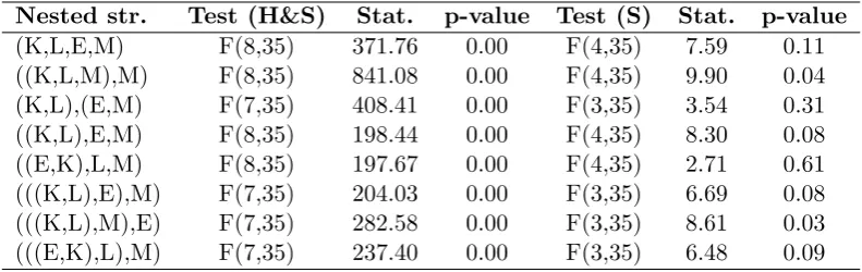
As separability restrictions are different for alternative nested structures, a Wald test on approximate separability allows to discriminate between them. With four inputs, the number of possible nested structures is very large. Especially if we consider nested CES functions composed by three levels of production, e.g. (((K, L), E), M). In the following of this section we only present results for the structures that we consider sensible from an economic point of view, i.e. those structures that make economic sense.7

Table 9 presents the Wald test results for the joint homogeneity and ap-proximate separability assumptions (which we expect to reject) and a test on approximate separability alone. Results indicate that among the structures

7_{For example, we do not include the ((E, L),(K, M)) structure as it would suggest that}

EK EL KL EM KL KM Agric., Hunting, Forestry and Fish. 1.447 -0.444 -0.098 -1.191 -0.092 0.456 Mining and Quarrying 1.247 -0.036 -0.232 -1.319 -0.302 0.420 Food, Beverages and Tobacco 1.450 -0.482 -0.137 -1.268 -0.222 0.446 Textiles, Leather and Footwear 1.400 -0.578 -0.139 -1.333 -0.113 0.444 Wood and of Wood and Cork 1.391 -0.740 -0.261 -1.461 -0.425 0.422 Pulp, Paper, Printing and Publ. 1.324 -0.316 -0.139 -1.364 -0.404 0.465 Chemical, Rubber, Plastics and Fuel 1.288 -0.047 -0.019 -1.334 -0.310 0.542 Other Non-Metallic Mineral 1.269 -0.468 -0.184 -1.415 -0.343 0.468 Basic Metals and Fabricated Metal 1.302 -0.367 -0.125 -1.418 -0.287 0.497 Machinery, Nec 1.407 -0.312 -0.105 -1.411 -0.240 0.436 Electrical and Optical Equipment 1.485 0.252 -0.032 -1.309 -0.115 0.515 Transport Equipment 1.265 0.129 -0.100 -1.189 0.106 0.456 Manufacturing Nec, Recycling 1.497 -0.599 -0.212 -1.370 -0.244 0.422 Electricity, Gas and Water Supply 1.476 -0.832 -0.226 -1.199 -0.247 0.370 Construction 1.376 -0.444 -0.171 -1.427 -0.408 0.496 Wholesale and Retail Trade 1.367 -0.429 -0.166 -1.312 -0.343 0.418 Hotels and Restaurants 1.293 -0.174 -0.071 -1.346 -0.375 0.448 Transport and Storage 1.338 -0.110 -0.043 -1.423 -0.372 0.535 Post and Telecommunications 1.356 -0.124 -0.040 -1.203 -0.318 0.401 Public Adm. and Defence 1.431 -0.578 -0.139 -1.030 -0.098 0.402 Education 1.397 -0.776 -0.200 -1.279 -0.313 0.396 Health and Social Work 1.384 -0.726 -0.212 -1.121 -0.307 0.390 Other Community Services 1.361 -0.681 -0.240 -1.393 -0.375 0.339

Table 7: Mean estimated Morishima elasticities of substitution by sector

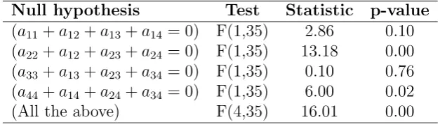
Null hypothesis Test Statistic p-value

(a11+a12+a13+a14= 0) F(1,35) 2.86 0.10 (a22+a12+a23+a24= 0) F(1,35) 13.18 0.00 (a33+a13+a23+a34= 0) F(1,35) 0.10 0.76 (a44+a14+a24+a34= 0) F(1,35) 6.00 0.02

(All the above) F(4,35) 16.01 0.00

Table 8: Wald tests on homogeneity for different nested structures

Nested str. Test (H&S) Stat. p-value Test (S) Stat. p-value (K,L,E,M) F(8,35) 371.76 0.00 F(4,35) 7.59 0.11 ((K,L,M),M) F(8,35) 841.08 0.00 F(4,35) 9.90 0.04 (K,L),(E,M) F(7,35) 408.41 0.00 F(3,35) 3.54 0.31 ((K,L),E,M) F(8,35) 198.44 0.00 F(4,35) 8.30 0.08 ((E,K),L,M) F(8,35) 197.67 0.00 F(4,35) 2.71 0.61 (((K,L),E),M) F(7,35) 204.03 0.00 F(3,35) 6.69 0.08 (((K,L),M),E) F(7,35) 282.58 0.00 F(3,35) 8.61 0.03 (((E,K),L),M) F(7,35) 237.40 0.00 F(3,35) 6.48 0.09

Table 9: Wald tests on homogeneity and separability (H&S) and separability alone (S) for different nested structures

6.2

Graphical analysis

Graphical analysis of Translog point elasticities could also provide an indica-tion on how far elasticities are from being constant. This analysis is based on the distribution of the Translog estimated substitution elasticities and on the prediction intervals constructed around each of them. They show the range inside which an estimated elasticities obtained from new values of inputs and output quantities for a certain sector will fall 95% of times.

An important evidence in favour of the CES functional form can be ob-tained looking at the distribution of the estimated elasticities. If the dis-tribution peaks around few values and is not uniformly distributed, i.e. the elasticity values remain quite stable across the sample, a constant elasticity is supported by the data and, hence, a CES specification. Also, the size of the prediction intervals helps to gauge how much the elasticities vary: if the interval is narrow, a new point elasticity is predicted to fall in that particular precise range.

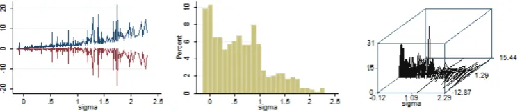
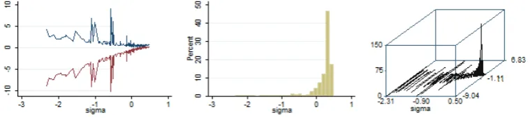
In the following of this section, we show three graphs for each elasticity: the first graph represents the lower and upper bounds of the interval for each point elasticity, the second shows the elasticities distributions and the third combines the two previous graphs in a surface graph. In this analysis we consider only the HES as they are the ones that are constant in a nested CES function. We control for outliers excluding the highest and lowest 10% of the estimated elasticities.

elas-ticities vary from approximately 1.08 and 1.5 but from Figure 1 we can see that most of the values lie between 1.08 and 1.3. Moreover, the prediction intervals around those values are quite narrow (the value of the lower and upper bounds of the interval in the interval 1.08 and 1.15 are approximately 0 and 2 respectively) indicating that the point elasticity variation is limited. The surface graph confirms this intuition showing a narrow peak around 1.1. The remaining elasticities show larger variation in the point elasticities distribution. Prediction intervals are in general quite narrow though, indi-cating that each point elasticities is well predicted. We can conclude that the graphical analysis is in line with the recommendation obtained from the formal nesting tests, i.e. the E-K elasticity is the “most constant”.

Figure 1: Translog estimated E-K Hicks elasticities graphical analysis

Figure 2: Translog estimated E-L Hicks elasticities graphical analysis

7

CES estimation

Figure 3: Translog estimated K-L Hicks elasticities graphical analysis

Figure 4: Translog estimated E-M Hicks elasticity graphical analysis

Figure 5: Translog estimated K-M Hicks elasticity graphical analysis

Figure 6: Translog estimated L-M Hicks elasticity graphical analysis

CES (Hoff, 2014) and the third on the estimation of the FOCs derived from a stepwise optimization procedure where a cost function based on the first the inner CES and then the one based complete nested CES are minimised (Chang, 1994;Prywes, 1986; van der Werf,2008; Baccianti,2013).

We use a direct estimation method and estimate the nested CES with a Maximum Likelihood estimator. We are aware that this is not the most efficient estimator given the econometric issues underlined by the diagnostic tests; however the obtained coefficients will be unbiased and consistent. The nested CES can be expressed with the following notation:8

lnQit=lnλ+γt+

σ σ−1ln

δX

σ−1

σ

it +δzL

σ−1

σ

it + (1−δ−δz)M

σ−1

σ

it

(3)

with

Xit=ln

δxE

σx−1

σx

it + (1−δx)K

σx−1

σx

it

_σxσx₋₁

(4)

whereλ∈[0,+∞) is the efficiency parameters, γ is a measure of techno-logical progress, δ ∈ (0,1), δx ∈ (0,1) and δz ∈ (0,1) are share parameters

and σ and σx are substitution elasticities. We assume that the nested CES

is characterised by constant returns to scale.

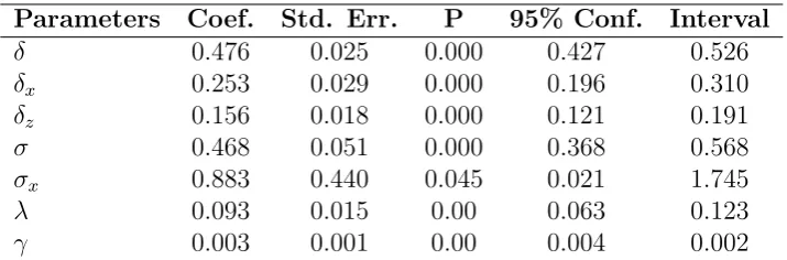
In Table 10we report the results of the Maximum Likelihood estimation regression. We can see that all regressors are significant at a 5% level and that they lie in the ranges predicted by the economic theory. The elasticity of substitution between energy and capital is equal to 0.883. This is in line with our previous findings as it falls in the estimated prediction interval. The elasticity of substitution between the energy and capital composite input and the remaining inputs is equal to 0.468.

8

Conclusions

In this paper, we contribute to the applied econometric literature on the sub-stitution relationships between inputs of production by estimating the elas-ticities of substitution between energy and other inputs. Our data are drawn from the EU-KLEMS database and include 23 UK industrial sectors for the period 19702005. In line with the cited literature, we employ a Translog

Parameters Coef. Std. Err. P 95% Conf. Interval

δ 0.476 0.025 0.000 0.427 0.526

δx 0.253 0.029 0.000 0.196 0.310

δz 0.156 0.018 0.000 0.121 0.191

σ 0.468 0.051 0.000 0.368 0.568

σx 0.883 0.440 0.045 0.021 1.745

λ 0.093 0.015 0.00 0.063 0.123

γ 0.003 0.001 0.00 0.004 0.002

Table 10: Maximum Likelihood estimation of the nested CES production function

functional form to describe our production function. Furthermore, we com-pute three different types of elasticities: the Hicks, Allen and Morishima elasticities. Our results suggest that energy and capital are substitutes in production.

We also contribute to the CGE literature by providing both an indication of the appropriate nested structure and the relative constant elasticities for UK production. In the paper, we check whether data support a nested CES representation of the production function. We use both empirical and graph-ical tests and we conclude that a nested structure of the form ((E,K),L,M) is the most appropriate to describe a CES production technology for the dataset under analysis. From the estimation of this nested CES, we obtain the constant elasticities of substitution which are equal to 0.88 and 0.47 for the inner and the outer nest respectively.

References

Allan, G., N. Hanley, P. McGregor, K. Swales, and K. Turner.

2007. “The impact of increased efficiency in the industrial use of energy: A computable general equilibrium analysis for the United Kingdom.”Energy Economics, 29(4): 779–798.

Apostolakis, B. E. 1990. “Energy-capital

substitutabil-ity/complementarity.”Energy Economics, 12(1): 48–58.

Baccianti, C.2013. “Estimation of sectoral elasticities of substitution along the international technology frontier.” ZEW Discussion Papers 13-092, ZEW - Zentrum fr Europische Wirtschaftsforschung/ Center for European Economic Research.

Baum, C. F. 2000a. “XTTEST2: Stata module to perform Breusch-Pagan

LM test for cross-sectional correlation in fixed effects model.” Statistical Software Components, Boston College Department of Economics, Decem-ber.

Baum, C. F. 2000b. “XTTEST3: Stata module to compute Modified Wald

statistic for groupwise heteroskedasticity.” Statistical Software Compo-nents, Boston College Department of Economics, October.

Baum, C. F., M. E. Schaffer, and S. Stillman. 2002. “IVREG2:

Stata module for extended instrumental variables/2SLS and GMM esti-mation.” Statistical Software Components, Boston College Department of Economics, April.

Berndt, E. R., and D. Wood. 1975. “Technology, prices and the derived

demand for energy.” The Review of Economics and Statistics, 57(3): 259– 268.

Blackorby, C., and R. Russell.1989. “Will the real elasticity of

substitu-tion please stand up? (a comparison of the Allen/Uzawa and Morishima elasticities).”The American Economic Review, 79(4): 882–888.

Burki, A., and M. U. H. Khan.2004. “Effects of allocative inefficiency on

resource allocation and energy substitution in Pakistan’s manufacturing.”

Chang, K.1994. “Capital-energy substitution and the multi-level CES pro-duction function.” Energy Economics, 16(1): 22–26.

Choi, I. 2001. “Unit root tests for panel data.” Journal of International

Money and Finance, 20(2): 249–272.

Christopoulos, D. K. 2000. “The demand for energy in Greek

manufac-turing.” Energy Economics, 22(5): 569–586.

Chung, J. W.1987. “On the estimation of factor substitution in the translog model.” The Review of Economics and Statistics, 69(3): 409–417.

Dargay, J. M. 1983. “The demand for energy industries manufacturing.”

The Review of Economics and Statistics, 85(1): 37–51.

Despotakis, K. A., and A. C. Fisher. 1988. “Energy in a regional

econ-omy: A computable general equilibrium model for California.” Journal of Environmental Economics and Management, 15(3): 313–330.

Driscoll, J., and A. Kraay. 1998. “Consistent covariance matrix

esti-mation with spatially dependent panel data.” Review of Economics and Statistics, 80: 549–560.

Field, B. C., and C. Grebenstein. 1980. “Capital-energy substitution

in U.S. manufacturing.” The Review of Economics and Statistics, 62(2): 207–212.

Fuss, M. A. 1977. “The demand for energy in Canadian manufacturing.”

Journal of Econometrics, 5(1): 89–116.

Garofalo, G. A., and D. Malhotra. 1988. “Aggregation of capital and

its substitution with energy.”Eastern Economic Journal, 14(3): 251–262.

Greene, W. H.2008.Econometric Analysis. Upper Saddle River, NJ:

Pren-tice Hall.

Griffin, J. M., and P. R. Gregory. 1976. “Intercountry translog model

Haller, S., and M. Hyland.2014. “Capital-energy substitution: Evidence from a panel of Irish manufacturing firms.”Energy Economics, 45(C): 501– 510.

Hertel, T. W., and T. D. Mount.1985. “The pricing of natural resources

in a regional economy.” Land Economics, 61(3): 229–243.

Hesse, D. M., and H. Tarkka. 1986. “The demand for capital, labor and

energy in European industry manufacturing before and after the oil price shocks.” The Scandinavian Journal of Economics, 88(3): 529–546.

Hisnanick, J. J., and B. L. Kyer. 1995. “Assessing a disaggregated

en-ergy input using confidence intervals around translog elasticity estimates.”

Energy Economics, 17(2): 125–132.

Hoechle, D. 2006. “XTSCC: Stata module to calculate robust standard

er-rors for panels with cross-sectional dependence.” Statistical Software Com-ponents, Boston College Department of Economics, November.

Hoechle, D.2007a. “Robust standard errors for panel regressions with cross-sectional dependence.” Stata Journal, 7(3): 281–32.

Hoechle, D. 2007b. “Robust standard errors for panel regressions with

cross-sectional dependence.” Stata Journal, 7(3): 281–312.

Hoff, A. 2014. “The linear approximation of the CES function with n input

variables.”Marine Resource Economics, 19(3): 295–306.

Hoyos, R. E. D., and V. Sarafidis.2006b. “XTCSD: Stata module to test

for cross-sectional dependence in panel data models.” Statistical Software Components, Boston College Department of Economics, June.

Hoyos, R. E. D., and V. Sarafidis. 2006a. “Testing for cross-sectional

dependence in panel-data models.” Stata Journal, 6(4): 482–496.

Kemfert, C. 1998. “Estimated substitution elasticities of a nested CES

Khiabani, N., and K. Hasani. 2010. “Technical and allocative inefficien-cies and factor elasticities of substitution: An analysis of energy waste in Iran’s manufacturing.” Energy Economics, 32(5): 1182–1190.

Kim, J., and E. Heo. 2013. “Asymmetric substitutability between energy

and capital: Evidence from the manufacturing sectors in 10 OECD coun-tries.” Energy Economics, 40(C): 81–89.

Kleibergen, F., and M. E. Schaffer. 2007. “RANKTEST: Stata module

to test the rank of a matrix using the Kleibergen-Paap rk statistic.” Sta-tistical Software Components, Boston College Department of Economics, August.

Koesler, S., and M. Schymura. 2015. “Substitution elasticities in a

con-stant elasticity of substitution framework: Empirical estimates using Non-linear Least Squares.”Economic Systems Research, 27(1): 101–121.

Koetse, M. J., H. L. de Groot, and R. J. Florax. 2008.

“Capital-energy substitution and shifts in factor demand: A meta-analysis.”Energy Economics, 30(5): 2236–2251.

Lagomarsino, E. 2017. “Are substitution elasticities constant? An

empiri-cal procedure to help discriminate between functional forms.” Mimeo.

Lecca, P., K. Swales, and K. Turner. 2011. “An investigation of issues

relating to where energy should enter the production function.”Economic Modelling, 28(6): 2832–2841.

Li, P., and A. Rose. 1995. “Global warming policy and the Pennsylvania

economy: A computable general equilibrium analysis.” Economic Systems Research, 7(2): 151–171.

Maddala, G. S., and S. Wu.1999. “A comparative study of unit root tests

with panel data and a new simple test.”Oxford Bulletin of Economics and Statistics, 61(S1): 631–652.

Medina, J., and J. Vega-Cervera. 2001. “Energy and the non-energy

Moghimzadeh, M., and K. O. Kymn. 1986. “Cost shares, own, and cross-price elasticities in U.S. manufacturing with disaggregated energy inputs.”The Energy Journal, 7(4): 65–80.

Nguyen, S., and M. Streitwieser.1999. “Factor substitution in U.S.

man-ufacturing: Does plant size matter?” Small Business Economics, 12(1): 41–57.

Norsworthy, J., and D. H. Malmquist. 1983. “Input measurement and

productivity growth in Japanese and U.S. manufacturing.” The American Economic Review, 73(5): 947–967.

Okagawa, A., and K. Ban. 2008. “Estimation of substitution elasticities

for CGE models.” Discussion Papers in Economics and Business 08-16, Osaka University, Graduate School of Economics and Osaka School of In-ternational Public Policy (OSIPP).

Ozatalay, S., S. Grubaugh, and T. Veach Long II. 1979. “Energy

substitution and national energy policy.”The American Economic Review, 69(2): 369–371.

Pedroni, P.2000. “Fully modified OLS for heterogeneous cointegrated

pan-els.” Department of Economics Working Papers 2000-03, Department of Economics, Williams College.

Perroni, C., and T. F. Rutherford. 1995. “Regular flexibility of nested

CES functions.”European Economic Review, 39(2): 335–343.

Pindyck, R. S. 1979. “Interfuel substitution and the industrial demand

for energy: An international comparison.” The Review of Economics and Statistics, 61(2): 169–179.

Prywes, M.1986. “A nested CES approach to capital-energy substitution.”

Energy Economics, 8(1): 22–28.

Roy, J., A. H. Sanstad, J. a. Sathaye, and R. Khaddaria. 2006.

“Substitution and price elasticity estimates using inter-country pooled data in a translog cost model.”Energy Economics, 28(5-6): 706–719.

Saunders, H. D. 2000. “Does predicted rebound depend upon

Schaffer, M. E. 2005. “XTIVREG2: Stata module to perform extended IV/2SLS, GMM and AC/HAC, LIML and k-class regression for panel data models.” Statistical Software Components, Boston College Department of Economics, November.

Schaffer, M. E., and S. Stillman. 2006. “XTOVERID: Stata module to

calculate tests of overidentifying restrictions after xtreg, xtivreg, xtivreg2, xthtaylor.” Statistical Software Components, Boston College Department of Economics, October.

StataCorp. 2013. “Stata Statistical Software: Release 13.” College Station,

TX: StataCorp LP.

Thompson, P., and T. G. Taylor. 1995. “The capital-energy

substi-tutability debate: A new look.” The Review of Economics and Statistics, 77(3): 565–569.

Turner, K. 2009. “Negative rebound and disinvestment effects in response

to an improvement in energy efficiency in the UK economy.” Energy Eco-nomics, 31(5): 648–666.

Turnovsky, M., M. Folie, and A. Ulph. 1982. “Factor substitutability

in Australian manufacturing with emphasis on energy inputs.” Economic Record, 58(1): 61–72.

van der Werf, E.2008. “Production functions for climate policy modeling:

An empirical analysis.”Energy Economics, 30(6): 2964–2979.

Wooldridge, J. M.2002.Econometric Analysis of Cross Section and Panel

Data. Cambridge, Massachusetts: The MIT Press.

Zha, D., and N. Ding. 2014. “Elasticities of substitution between energy

and non-energy inputs in China power sector.”Economic Modelling, 38(C): 564–571.

Zha, D., and D. Zhou.2014. “The elasticity of substitution and the way of

Appendices

Code Sectors

AtB AGRICULTURE, HUNTING, FORESTRY AND FISHING

C MINING AND QUARRYING

15t16 FOOD , BEVERAGES AND TOBACCO

17t19 TEXTILES, TEXTILE , LEATHER AND FOOTWEAR

20 WOOD AND OF WOOD AND CORK

21t22 PULP, PAPER, PAPER , PRINTING AND PUBLISHING

23t25 CHEMICAL, RUBBER, PLASTICS AND FUEL

26 OTHER NON-METALLIC MINERAL

27t28 BASIC METALS AND FABRICATED METAL

29 MACHINERY, NEC

30t33 ELECTRICAL AND OPTICAL EQUIPMENT

34t35 TRANSPORT EQUIPMENT

36t37 MANUFACTURING NEC; RECYCLING

E ELECTRICITY, GAS AND WATER SUPPLY

F CONSTRUCTION

G WHOLESALE AND RETAIL TRADE

H HOTELS AND RESTAURANTS

60t63 TRANSPORT AND STORAGE

64 POST AND TELECOMMUNICATIONS

L PUBLIC ADM. AND DEFENCE; COMPULSORY SOCIAL SECURITY

M EDUCATION

N HEALTH AND SOCIAL WORK

O OTHER COMMUNITY, SOCIAL AND PERSONAL SERVICES