arXiv:1609.08367v1 [cs.LO] 27 Sep 2016
HELLE HVID HANSEN, CLEMENS KUPKE, AND JAN RUTTEN Delft University of Technology and Centrum Wiskunde & Informatica, Amsterdam e-mail address: [email protected]
University of Strathclyde
e-mail address: [email protected]
Centrum Wiskunde & Informatica, Amsterdam, and Radboud University Nijmegen e-mail address: [email protected]
Abstract. Streams, or infinite sequences, are infinite objects of a very simple type, yet they have a rich theory partly due to their ubiquity in mathematics and computer science. Stream differential equations are a coinductive method for specifying streams and stream operations, and their theory has been developed in many papers over the past two decades. In this paper we present a survey of the many results in this area. Our focus is on the classification of different formats of stream differential equations, their solution methods, and the classes of streams they can define. Moreover, we describe in detail the connection between the so-called syntactic solution method and abstract GSOS.
1. Introduction
Streams, or infinite sequences, are infinite objects of a very simple type, yet they have a rich theory partly due to their ubiquity. Streams occur as numerical expansions, data sequences, formal power series, limit sequences, dynamic system behaviour, formal languages, ongoing computations, and much more.
Defining thestream derivative of a stream σ= (σ(0), σ(1), σ(2), . . .) by σ′ = (σ(1), σ(2), σ(3), . . .)
and theinitial value ofσbyσ(0), one can develop acalculus of streams in close analogy with classical calculus in mathematical analysis. Notably, using the notions of stream derivative and initial value, we can specify streams by means of stream differential equations.
For instance, the stream differential equation σ(0) = 1, σ′ = σ has the stream σ =
(1,1,1, . . .) as its unique solution, and σ(0) = 1, σ′ =σ+σ, where + is the elementwise
1998 ACM Subject Classification: F.1.1, F.3.2, F.4.3.
Key words and phrases: streams, behavioural differential equations, coinduction, coalgebra, linear sys-tems, context-free streams, automatic sequences, bialgebra.
Supported by NWO-Veni grant 639.021.231. Supported by EPSRC grant EP/N015843/1.
LOGICAL METHODS
IN COMPUTER SCIENCE DOI:10.2168/LMCS-???
c
Hansen, Kupke, and Rutten Creative Commons
addition of two streams, defines the stream (20,21,22, . . .) . Similarly, we can specify stream
functions. For example, f(σ)(0) = σ(0), f(σ)′ = f(σ′′) (this time using second-order derivatives) defines the function f(σ) = (σ(0), σ(2), σ(4), . . .). In these examples, it is easy to see that the stream differential equations have a unique solution. But how about τ(0) = 0, τ′ =f(τ)? A moment’s thought reveals that this equation has several solutions, e.g. τ = (0,0,0, . . .) and τ = (0,0,1,1,1, . . .). But what is the difference between this equation and the previous ones? How can we ensure the existence of unique solutions? Which classes of streams can be defined using a finite amount of information? These questions have been studied by several authors in many different contexts in recent years, and have led to notions such as rational streams, context-free streams, and new insights into automatic and regular sequences.
In this paper, we present an overview of the current state-of-the-art in formats and solu-tion methods for stream differential equasolu-tions. The theoretical basis for stream differential equations is given by coalgebra [56], but our aim is to give an elementary and self-contained overview. We consider our contribution to be a unified and uniform presentation of results which are collected from many different sources. As modest new insights, we mention the results on the expressiveness of non-standard formats in Section 7. Another contribution which can be considered new, is the detailed analysis of the connection between the syntac-tic method and abstract GSOS (in Section 9) This connection is rather obvious to readers familiar with abstract GSOS, but probably less so to the uninitiated reader.
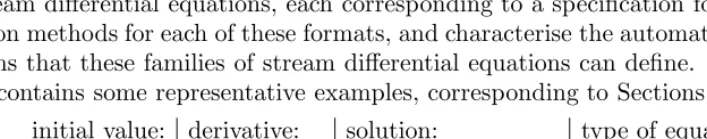
[image:2.612.89.443.428.497.2]Overview: We start by giving an informal introduction to stream differential equations in Section 2, and in Section 3 we provide some basic definitions regarding automata and stream calculus. Next, in Sections 4 through 7, we shall study in more detail various types of stream differential equations, each corresponding to a specification format. We describe solution methods for each of these formats, and characterise the automata and the classes of streams that these families of stream differential equations can define. The following little table contains some representative examples, corresponding to Sections 4 through 7:
initial value: derivative: solution: type of equation: σ(0) = 1 σ′=σ (1,1,1, . . .) simple
σ(0) = 1 σ′=σ+σ (20,21,22, . . .) linear
σ(0) = 1 σ′=σ×σ Catalan numbers context-free/algebraic
σ(0) = 1 dXd (σ) =σ 0!1,1!1,2!1,3!1,4!1, . . .
non-standard
(For the definition of the convolution product × see (2.6) in Section 2; the non-standard derivative dXd is defined in Example 7.1.)
In Section 8, we describe a concrete syntactic solution method for a large class of well-formed stream differential equations, including all those that we discussed in Sections 4-6. Finally, in Section 9, a more general, categorical perspective on the theory of stream differential equations is presented. In particular, this section places streams and automata in a more general context of algebras, coalgebras and so-called distributive laws. Note that this is the only section that requires some basic knowledge of category theory. In Section 10, we briefly discuss connections with other methods for representing streams, such as recurrence relations, generating functions and so on.
for examples and motivations. Section 9 can be skipped by readers who are mainly interested in concrete specification formats. Section 10 relies on Sections 2-7.
Related work: Here we mention the most important origins of the results in this paper. A more extensive discussion of related work is found in Section 10. Stream differential equations [60] came about as a special instance of behavioural differential equations, for formal power series, which were introduced in [58]. Motivation came from the coalgebraic perspective on infinite data structures, in which streams are a canonical example, but also from work on language dervatives in classical automata theory, notably [16] and [17]. The idea of developing a calculus of streams in close analogy to analysis was further inspired by the work on classical calculus in coinductive form in [52]. The classification of stream differential equations into the families of simple, linear and context-free systems stems from our joint work with Marcello Bonsangue and Joost Winter, in [13] and [69], on classifications of behavioural differential equations for streams, languages and formal power series. The results on non-standard stream calculus come from [40, 39], and the examples on automatic and regular sequences from [41] and [28], respectively.
Acknowledgements: It should be clear from the many references to the literature that our paper builds on the work of many others. We are, in particular, much indebted to Marcello Bonsangue and Joost Winter for many years of fruitful collaboration on stream differential equations. A large part of the work presented here was developed in joint work with them. We are also grateful to many other colleagues, with whom we have worked together in different ways on ideas relating to streams, including: Henning Basold, Filippo Bonchi, J¨org Endrullis, Herman Geuvers, Clemens Grabmayer, Dimitri Hendriks, Bart Jacobs, Bartek Klin, Jan-Willem Klop, Dorel Lucanu, Larry Moss, Milad Niqui, Grigore Rosu, Jurriaan Rot, Alexandra Silva, Hans Zantema.
Contents
1. Introduction 1
2. Stream Differential Equations 4
2.1. Basic definitions 4
2.2. Simple examples 5
2.3. Stream operations 5
2.4. Higher-order examples 6
3. Stream Automata and Stream Calculus 7
3.1. Stream Automata and coinduction 7
3.2. Stream Calculus 9
4. Simple Specifications 10
5. Linear Specifications 12
5.1. Linear equation systems 12
5.2. Linear stream automata 12
5.3. Matrix solution method 14
6. Context-free Specifications 19
6.1. Context-free equation systems 19
6.2. Solutions and characterisations 20
7. Non-standard Specifications 22
7.1. Stream representations 22
7.3. Stream specifications for automatic sequences 27
8. The Syntactic Method 29
8.1. Terms and algebras 30
8.2. Stream GSOS definitions 31
8.3. Causal stream operations 36
8.4. Causality and productivity 37
8.5. Simple/linear/context-free stream specifications revisited 37
9. A General Perspective 39
9.1. Coalgebras for a functor 40
9.2. Algebras for a monad 40
9.3. Bialgebras for a distributive law 41
9.4. The Syntactic Method via Abstract GSOS 42
9.5. Solving systems of equations 45
10. Discussion and Related Work 46
10.1. Other Specification Methods 46
10.2. Related Work 47
References 49
2. Stream Differential Equations
In this section, we present several examples ofstream differential equations (SDEs)and their solutions. For now the purpose is to get familiarised with the notation of SDEs. Detailed proofs and solution methods are presented later.
We start by introducing notation and basic definitions on streams.
2.1. Basic definitions. A stream over a given set A is a function σ: N → A from the natural numbers toA, which we will sometimes write as
σ= (σ(0), σ(1), σ(2), . . .) The set of all streams over Ais denoted by
Aω ={σ |σ:N→A}
Given a stream σ ∈ Aω, we define the initial value of σ as σ(0), and the derivative of σ as the stream σ′ = (σ(1), σ(2), σ(3), . . .). For a ∈ A and σ ∈ Aω, we define a:σ =
(a, σ(0), σ(1), σ(2), . . .). Higher order derivatives σ(n) are defined inductively for alln∈N
by:
σ(0) =σ σ(n+1) = (σ(n))′
2.2. Simple examples. Stream differential equations define a stream in terms of its initial value and its derivative(s). As a first elementary example, consider
σ(0) = 1, σ′ =σ. (2.1)
which has the stream ones= (1,1,1, . . .) as the unique solution.
For a slightly more interesting example consisting of two SDEs over two stream vari-ables, consider
σ(0) = 1, σ′ =τ
τ(0) = 0, τ′ =σ
(2.2)
whose solution is σ= (1,0,1,0, . . .) andτ = (0,1,0,1, . . .).
In the above SDEs, derivatives given by a stream variable. Such SDEs are called simple, and in Section 4, we will characterise the class of streams that can be specified by finite systems of simple equations. More generally, we will consider SDEs involving not only variables, but also operations on streams.
2.3. Stream operations. We illustrate how to define stream operations, and at the same time introduce a bit of stream calculus. Stream calculus is usually defined for streams over the real numbersR, but most definitions hold for more general data domains A.
Consider the set Aω of streams over a ring (A,+,−,·,0,1). The stream differential equation:
(σ+τ)(0) = σ(0) +τ(0), (σ+τ)′ = σ′+τ′ (2.3)
defines the element-wise addition of two streams, that is, for all σ, τ ∈Aω,
(σ+τ)(n) =σ(n) +τ(n) for all n∈N. (2.4) (Note that we use the same symbol to denote addition inA and addition of streams. The typing should be clear from the context.)
Similarly, one can define the element-wise multiplication with a scalar a∈A with the SDE:
(a·σ)(0) =a·σ(0), (a·σ)′ =a·σ′. (2.5) wherea·σ(0) denotes multiplication inA. It follows that, for allσ∈Aω,
(a·σ)(n) =a·σ(n) for all n∈N.
Clearly, any element-wise operation on streams can be defined in a similar manner. An ex-ample of a non-element-wise operation is theconvolution productof streams given explicitly by:
(σ×τ)(n) =
n X
k=0
σ(k)·τ(n−k) for all n∈N (2.6)
which is defined by the SDE
(σ×τ)(0) =σ(0)·τ(0), (σ×τ)′ = (σ′×τ) + ([σ(0)]×τ′) (2.7)
where fora∈A,
[a](0) =a, [a]′ = [0] (2.8)
Note that the stream [1] = (1,0,0,0, . . .) is the identity for the convolution product, that is,σ×[1] = [1]×σ =σ.
Using the convolution product, and takingA=Zwe can form the following SDE:
σ(0) = 1, σ′=σ×σ (2.9)
It defines the streamσ = (1,1,2,5,14,42,132,429,1430, . . .) of Catalan numbers, cf. [13]. WhenAis a field such as the reals R, some streamsσ have an inverseσ−1 with respect to convolution product, that is, σ×σ−1 =σ−1×σ = [1]. By taking initial value on both sides we find that the inverse should satisfy (σ×σ−1)(0) = 1 and hence by the definition of convolution product,σ−1(0) = 1/σ(0) which exists only if σ(0)6= 0 in A. Similarly, taking
derivatives on both sides and rearranging, we find the following SDE:
σ−1(0) = 1/σ(0), (σ−1)′ = [−1/σ(0)]×σ′×σ−1 (2.10)
2.4. Higher-order examples. Just as with classical differential equations, SDEs can also be higher-order. For instance, the second-order SDE
σ(0) = 0, σ′(0) = 1, σ′′=σ′+σ (2.11) (with + as defined above) defines the stream of Fibonacci numbersσ= (0,1,1,2,3,5,8, . . .). Annth order SDE can always be represented as a system ofnfirst-order SDEs. For example, the Fibonacci stream is equivalently defined as the solution for σ in
σ(0) = 0, σ′=τ
τ(0) = 1, τ′=τ+σ (2.12)
A similar example is given by
σ(0) = 1, σ′ = σ
τ(0) = 0, τ′ = τ+σ (2.13)
We know already thatonesis a solution forσ (cf. equation (2.1)). Hence (2.13) is equivalent to
τ(0) = 0, τ′ =τ +ones (2.14)
which hasτ = (0,1,2,3,4, . . .) as its unique solution.
A slightly more involved example is given by the stream γ of Hamming numbers (or regular numbers) which consists of natural numbers of the form 2i3j5k fori, j, k ≥0 in
in-creasing order (cf. [18, 71]). The first part ofγlooks like (1,2,3,4,5,6,8,9,10,12,15,16, . . .). The streamγ can be defined by the following SDE:
γ(0) = 1, γ′ = (2·γ)k((3·γ)k(5·γ)) (2.15) wheren·γ,n∈N, is the scalar multiplication defined as in (2.5) andkis themerge operator defined by
(σkτ)(0) =
σ(0) if σ(0)< τ(0)
τ(0) if σ(0)≥τ(0) (σkτ)′ =
σ′kτ if σ(0)< τ(0)
σ′kτ′ if σ(0) =τ(0) σkτ′ if σ(0)> τ(0)
(2.16)
That is,k merges two streams into one by taking smallest initial values first, and removing duplicates.
3. Stream Automata and Stream Calculus
We will show how one can prove the existence of unique solutions to SDEs by using the notions of stream automata and coinduction.
3.1. Stream Automata and coinduction. Streams can be represented by so-called stream automata. Astream automaton (with output in A) is a pairhX, si whereX is a set (called the state space, or the carrier) and s = ho, di:X → A×X is a function that maps each x ∈X to a pair consisting of an output value o(x) ∈A and a unique next state d(x) ∈X (corresponding to the derivative). We will write x−→a y when o(x) =a and d(x) = y. A small example of a stream automaton is given in Figure 1. (In categorical terms, a stream
x0 0 //x1 1
)
)x
2 0
i
i x3
0
Figure 1: Stream automaton withX={x0, x1, x2, x3} and A={0,1}.
automaton is a coalgebra for the functorF onSet defined byF X =A×X, cf. Section 9.) Intuitively, a statexin a stream automatonhX,ho, diirepresents the stream of outputs that can be observed by following the transitions starting inx:
(o(x), o(d(x)), o(d(d(x)), o(d(d(d(x)))), . . .)
This stream is called the (observable) behaviour of x. For example, the behaviour of the state x0 in Figure 1 is the stream (0,1,0,1, . . .). We will now characterise behaviour using
the notion of homomorphism and finality.
A homomorphism of stream automata is a function between state spaces that pre-serves outputs and transitions. Formally, a functionf:X1 →X2 is a homomorphism from
hX1,ho1, d1iito hX2,ho2, d2iiif and only if, for all x∈X1,
o1(x) =o2(f(x)) andf(d1(x)) =d2(f(x)),
or equivalently, if and only if, the following diagram commutes:
X1 ho1,d1i
f
/
/X2 ho2,d2i
A×X1 idA×f
/
/A×X2
where idA denotes the identity map on A.
The set of streams Aω is itself a stream automaton under the map ζ:σ 7→ hσ(0), σ′i, and it is moreover final which means that for any stream automaton ho, di:X → A×X there is a unique stream homomorphism [[−]] :X→Aω (called the final map) into hAω, ζi:
X
∀ho,di
∃![[−]]
/
/Aω
ζ
By the commutativity of the above diagram, we find that
[[x]] = (o(x), o(d(x)), o(d(d(x)), o(d(d(d(x)))), . . .)
is indeed the observable behaviour ofx∈X. The final map [[−]] is therefore often referred to as thebehaviour map. Note that by uniqueness, the final map fromhAω, ζi to itself must be the identity homomorphism, that is, for allσ ∈Aω:
[[σ]] =σ. (3.1)
It can now easily be verified that for the stream automaton in Figure 1, the behaviour map is:
[[x0]] = [[x2]] = (0,1,0,1, . . .)
[[x1]] = (1,0,1,0, . . .)
[[x3]] = (0,0,0,0, . . .)
The universal property of the final stream automaton yields a coinductive definition principle and a coinductive proof principle, both are often referred to as coinduction. In this paper we will make extensive use of both.
A mapf:X →Aω is said to bedefined by coinduction, if it is obtained as the unique homomorphism into the final stream automaton. In practice, such an f is obtained by equippingX with a suitable stream automaton structure and using the finality of hAω, ζi.
A proof by coinduction is based on the notion of bisimulation. Let hX1,ho1, d1ii and
hX2,ho2, d2iibe stream automata. A relation R⊆X1×X2 is astream bisimulation if for
all hx1, x2i ∈R:
o1(x1) =o2(x2) and hd1(x1), d2(x2)i ∈ R. (3.2)
Two statesx1 and x2 are said to bebisimilar, written x1∼x2, if they are related by some
stream bisimulation. We list a few well known facts about stream bisimulations, cf. [58]. Lemma 3.1. Let hX1, s1i and hX2, s2i be stream automata.
(1) If Ri ⊆X1×X2, i∈I, are stream bisimulations then Si∈IRi is a bisimulation. (2) The bisimilarity relation ∼ ⊆X1×X2 is the largest bisimulation between hX1, s1i
tohX2, s2i.
(3) Iff:X1→X2 is a stream homomorphism, then its graph R={hx, f(x)i |x∈X1} is a stream bisimulation.
The main result regarding bisimilarity is stated in the following theorem. Theorem 3.2. For all stream automatahXi, sii and all xi ∈Xi, i= 1,2,
x1 ∼x2 ⇐⇒ [[x1]] = [[x2]] Consequently, by (3.1), for all streams σ, τ ∈Aω,
σ ∼τ ⇐⇒ σ=τ
From Theorem 3.2 we get the coinductive proof principle: to prove that two streams are equal it suffices to show that they are related by a bisimulation relation.
Finally, we also need the notions of subautomaton and minimal automaton. A stream automaton hY, ti is asubautomaton of hX, si if Y ⊆X and the inclusion map ι:Y →X is a stream homomorphism, which means thatt=s↾Y. Given a stream automatonhX, si, the subautomaton generated byY0 ⊆Xis the subautomatonhY, tiobtained by closingY0 under
injective. Note that due to Theorem 3.2, every subautomaton of the final stream automaton is minimal.
Referring to the automaton in Figure 1, an example of a stream bisimulation is given by {(x0, x2),(x1, x1),(x2, x2)}. It follows from Theorem 3.2 that [[x0]] = [[x2]].
3.2. Stream Calculus. In this short section, we introduce some further preliminaries on stream calculus that we will be using in the remainder of the paper. As we have seen in Section 2.3, any operation onA can be lifted element-wise to an operation on Aω. In fact,
any algebraic structure on A lifts element-wise to Aω. (We show this in a more abstract setting in Section 9.5.2.) But we are not only interested in element-wise operations. We will use that if Ais a commutative ring, then also
(Aω,+,−,×,[0],[1])
is a commutative ring, cf. [58, Thm.4.1]. Similarly, ifA is a field, thenAω is a vector space over A with the operations of scalar multiplication and addition.
Table 1 summarises the SDEs defining the stream calculus operations on Aω most of which were already introduced in Section 2.3. The fact that these SDEs have unique solutions will follow from the results in Section 8.
derivative: initial value: name:
[a]′ = [0] [a](0) =a constant [a], a∈A
(σ+τ)′ =σ′+τ′ (σ+τ)(0) =σ(0) +τ(0) sum
(a·σ)′ =a·(σ′) (a·σ)(0) =a·σ(0) scalar multiplication
(−σ)′ =−(σ′) (−σ)(0) =−σ(0) minus
(σ×τ)′ = (σ′×τ) + ([σ(0)]×τ′) (σ×τ)(0) =σ(0)·τ(0) convolution product (σ−1)′ =−[σ(0)−1]×σ′×σ−1 (σ−1)(0) =σ(0)−1 convolution inverse
Table 1: Operations of stream calculus. Recall (from Section 2.3) that convolution inverse is defined only if σ(0) is an invertible element ofA. In the case A is a field this is equivalent withσ(0)6= 0, and as usual, we will often write στ forσ×τ−1.
We further add to our stream calculus the constant stream
X= (0,1,0,0,0, . . .) defined by X(0) = 0, X′ = [1].
Multiplication byX acts as “stream integration” (seen as an inverse to stream derivative) since
(X×σ)′ =σ This follows from the fact that, for all σ∈Aω,
X×σ = σ×X = (0, σ(0), σ(1), σ(2), . . .)
This leads to the very usefulfundamental theorem of stream calculus [58, Thm. 5.1]. Theorem 3.3. For everyσ ∈Aω, σ = [σ(0)] + (X×σ′).
Proof. For all σ, we have: σ = (σ(0), σ(1), σ(2), . . .)
We conclude this section by an enhancement of the bisimulation proof method. The general result behind the soundness of this method is described in Section 9.3.
Definition 3.4 (bisimulation-up-to). Let Σ denote a collection of stream operations. A relation R⊆Aω×Aω is a(stream) bisimulation-up-to-Σ if for all (σ, τ)∈R:
σ(0) =τ(0) and (σ′, τ′)∈R,¯ where ¯R⊆Aω×Aω is the smallest relation such that
(1) R⊆R¯
(2) { hσ, σi |σ∈Aω} ⊆R¯
(3) ¯R is closed under the (element-wise application of) operations in Σ. (For instance, if Σ contains addition andhα, βi,hγ, δi ∈R¯ then hα+γ, β+δi ∈R.)¯
We writeσ ∼Σ τ if there exists a bisimulation-up-to-Σ containing hσ, τi.
[image:10.612.220.311.553.607.2]Theorem 3.5(coinduction-up-to). Let Σbe a subset of the stream calculus operations from Table 1. We have:
σ∼Σ τ ⇒ σ =τ (3.3)
Proof. IfR is a bisimulation-up-to-Σ, then ¯R can be shown to be a bisimulation relation by structural induction on its definition. The theorem then follows by Theorem 3.2.
4. Simple Specifications
In Sections 4-6, we will characterise the classes of streams, i.e. subsets of Aω, that arise as
the solutions to finite systems of SDEs over varying algebraic structures/signatures. We start by defining the most simple type of systems of SDEs. LetA be an arbitrary set. A simple equation system over a set (of variables) X ={xi |i∈ I} is a collection of
SDEs, one for each xi ∈X, of the form
xi(0) = ai, x′i = yi;
where ai ∈A and yi ∈ X for alli ∈I. We call a simple equation system over X finite, if
X is finite. The SDEs in equations (2.1) and (2.2) are examples of finite simple equation systems. Note that any streamσ is the solution of theinfinite simple equation system over X={xn|n∈N} defined by: xn(0) =σ(n) andx′n=xn+1, for all n∈N.
A simple equation system corresponds to a map e:X → A×X, i.e., to a stream automaton with state space X. Asolution of e:X→A×X is an assignmenth:X →Aω of variables to streams that preserves the equations: h(xi) = ai and h(xi)′ = h(yi) for all
i∈I. This holds exactly when the following diagram commutes:
X
e
h
/
/Aω
ζ
A×XidA×h//A×Aω
In other words, solutions are stream homorphisms fromhX, eito the final stream automaton. By coinduction, solutions to simple equation systems exist and are unique. We will also say that a stream σ∈Aω is a solution of eif σ=h(x) for some x∈X, in which case we calle a specification ofσ.
We state the result explicitly to make clear the analogue with the results on linear and context-free specifications that will be discussed in Sections 5 and 6.
Proposition 4.1. The following are equivalent for all streams σ ∈Aω. (1) σ is the solution of a finite simple equation system.
(2) σ generates a finite subautomaton of the final stream automaton. (3) σ is eventually periodic, i.e., σ(k)=σ(n) for some k, n∈N with k < n.
Proof. 1⇒2: Let h:X → Aω be a solution of the finite e:X →A×X and σ=h(x) for some x ∈X. The subautomaton generated by σ is contained in the image h(X) which is finite, sinceX is finite.
2⇒ 3: The subautomaton generated by σ has as its state set {σ(k) |k ∈N} which is
finite by assumption. Consequently, there arek, n∈N such thatσ(k)=σ(n) and k < n. 3 ⇒ 1: Assume that σ(k) = σ(n) for k < n ∈ N. Let X = {x
0, . . . , xn−1} and define
e:X →A×X, for all i= 0, . . . , n−2, by
e(xi) =hσ(i), xi+1i
and by e(xn−1) =hσ(n−1), xki. Now σ=h(x0) where h is the unique solution ofe.
Eventually periodic streams constitute some of the simplest infinite objects that have a finite representation. Such finite representations make it possible to compute with and reason about infinite objects. We provide a couple of examples.
Example 4.2 (Rational numbers in binary). Let 2 ={0,1}denote the set of bits. Rational numbers with odd denominator, that is, elements of Qodd = {q = 2mn+1 | n, m ∈ Z}, can be represented as eventually periodic bitstreams. The representation B: Qodd → 2ω is obtained by coinduction via the following stream automaton structure on Qodd:
o(q) =nmod 2, d(q) = (q−o(q))/2
For example, the finitary representation of the number175 can be found by computing output and derivatives leading to the following stream automaton:
17 5
1
/
/ 6
5 0
/
/ 3
5 1
/
/ −1
5 1
/
/ −3
5 1
/
/ −4
5 0
/
/ −2
5
0
h
h
Hence,B(175) = 101(1100)ω. Such base 2 expansions allow for efficient implementations of arithmetic operations, cf. [31].
Example 4.3 (Regular languages over one-letter alphabet). A bitstream σ ∈ 2ω
corre-sponds to a language L⊆ P(A∗) over a one-letter alphabetA={a} via: an∈L ⇐⇒ σ(n) = 1, for alln∈N.
For example, the language L={an|n= 1 + 3k, k∈N}is represented by the state 0 in the
stream automaton:
0 0 //1 1 //2
0
d
5. Linear Specifications
Equations (2.12) and (2.13) in Section 2 are examples of linear equation systems: the righthand side of each SDE is a linear combination of the variables on the left. We will now study this type of systems in more detail.
Throughout this section we assume A is a field. The set Aω then becomes a vector space overA by defining scalar multiplication and vector addition pointwise, as in Table 1. We denote by V(X) the set of all formal linear combinations over X, i.e.,
V(X) ={a1x1+. . .+anxn|ai ∈A, xi ∈X, ∀i: 1≤i≤n}
or equivalently, V(X) is the set of all functions from X to A with finite support. In fact,
V(X) is itself a vector space over A by element-wise scalar multiplication and sum, and it is freely generated by X. That means X is a basis for V(X), and hence every linear map fromV(X) to a vector spaceW is determined by its action onX. More precisely, for every function f:X → W there is a unique linear map f♯:V(X) → W extending f, which is
defined by:
f♯(a1x1+. . .+anxn) =a1f(x1) +. . .+anf(xn).
We note that the linear extension id♯Aω:V(Aω) → Aω of the identity map id : Aω → Aω
gives the evaluation of formal linear combinations in the vector spaceAω.
5.1. Linear equation systems. A linear equation system over a setX={xi |i∈I}is a
collection of SDEs, one for eachxi∈X, of the form
xi(0) = ai, x′i = yi;
whereai ∈A andyi∈ V(X) for alli∈I. In other words, a linear equation system is a map
e=ho, di: X→A× V(X).
Again, we say thateis finite, ifXis finite. Asolution ofeis an assignmenth:X→Aωthat preserves the equations, that is, for allxi ∈X ={x1, . . . , xn}, if d(xi) =a1x1+. . .+anxn,
then
h(xi)(0) =o(xi) and h(xi)′ =a1·h(x1) +· · ·+an·h(xn)
In the remainder of this section, we give two ways of solving finite linear equation systems and characterise their solutions. The first uses coinduction for automata over vector spaces — here we will see that any linear equation system has a unique solution, and solutions to finite linear equation systems are exactly the streams that generate a finite-dimensional subspace. The second uses stream calculus and yields a matrix solution method which in turn shows that solutions to finite linear equation systems are exactly the rational streams.
To illustrate the construction, consider the two-dimensional linear equation system from (2.13), repeated here:
x1(0) = 1, x′1 = x1
x2(0) = 0, x′2 = x1+x2 (5.1)
It corresponds to the following weighted stream automaton (where a state is underlined if the output is 1, otherwise the output is 0):
x1
1 %% oo 1 x2 1
h
h
Let us try to construct a stream automaton for the solution of x2 by inductively applying
(5.1) and the definition of + (cf. (2.3)):
x2 −→0 x1+x2 1
−→ x1+ (x1+x2) = 2·x1+x2
2
−→ x1+ (x1+ (x1+x2)) = 3·x1+x2 3
−→ . . .
We notice two things: First, the stream behaviour ofx2 indeed consists of the sequence of
natural numbersnats= (0,1,2,3,4,5, . . .). Second, the states of this stream automaton are not stream variables, but linear combinations of the stream variables x1 and x2.
Remark 5.1. The above example also shows that for streams over the field A=R, if the coefficients of the linear system are integers, then the solutions will be streams of integers, since all initial values will be computed using only multiplication and addition of integers.
The above example motivates the following definition.
Definition 5.2. Alinear stream automaton is a stream automaton over vector spaces, i.e., it is a pair of mapsho, di:V →A×V whereV is a vector space overA, ando:V →A and d:V →V are linear maps. Note that the pairingho, diis again linear. A homomorphism of linear stream automata is a map between the state vector spaces which is both linear and a homomorphism of stream automata.
Solutions to a linear equation system will now be obtained by coinduction, for linear stream automata, using the following lemma.
Lemma 5.3. We have:
(1) A linear equation systeme: X→A×V(X)corresponds to a linear stream automaton
e♯:V(X)→A× V(X)
(2) The final stream automaton is also a final linear stream automaton.
Proof. (1): SinceAis a vector space over itself, A× V(X) is a (product) vector space, and we obtain e♯:V(X) →A× V(X) as the linear extension of e. Note that e♯=ho♯, d♯i.
(2): The initial value and derivative maps are linear:
(a·σ+b·τ)(0) = a·σ(0) +b·τ(0) (a·σ+b·τ)′ = a·σ′+b·τ′
Hence hAω, ζi is a linear stream automaton. Moreover, for any linear stream automaton
linear, since for all v, w∈V,a, b∈A and n∈N, [[a·v+b·w]](n) = o(dn(a·v+b·w))
= a·o(dn(v)) +b·o(dn(w)) (by linearity ofoand d) = a·[[v]](n) +b·[[w]](n)
Hence [[−]] is also the unique homomorphism of linear stream automata intohAω, ζi. Proposition 5.4. Every linear equation system has a unique solution.
Proof. Applying Lemma 5.3 and the coinduction principle for linear stream automata, we obtain for each linear equation systemho, di: X→A× V(X) a unique linear stream homo-morphismg:V(X)→Aω, as shown in the following picture whereηX:X→ V(X) denotes
the inclusion of the basis vectors intoV(X):
X
ho,di
ηX
/
/V(X)
ho♯,d♯i
z
z
✉✉✉✉ ✉✉✉✉
✉✉✉
g
/
/Aω
ζ
A× V(X) idA×g //A×Aω
(5.2)
The composition g◦ηX =g↾X:X →Aω is a solution of ho, di by the linearity of g. To see
this, suppose thatd(xi) =a1x1+. . .+anxn forxi ∈X. We then have:
g↾X(xi)′ = g(d(xi)) =g(a1x1+. . .+anxn)
= a1g↾X(x1) +. . .+ang↾X(xn)
We note that for finiteX, the linear homomorphismg:V(X) →Aω can be represented by a finite dimensional matrix with rational streams as entries, similar to the one in (5.4) of the next subsection; see [63] or [11] for details.
We can now state the first characterisation of the solutions to finite linear equation systems.
Proposition 5.5. The following are equivalent for all streams σ ∈Aω: (1) σ is the solution of a finite linear equation system.
(2) σgenerates a finite-dimensional subautomaton of the final linear stream automaton. Proof. For the direction 1 ⇒ 2: Let σ be a solution to a finite e:X → A× V(X). Let
hZσ, ζσi be the linear subautomaton generated byσ in the final linear automaton, i.e., the
state space Zσ is the subspace generated by the derivatives of σ. Since V(X) is
finite-dimensional, so is its final image g(V(X)), and since Zσ is a subspace of g(V(X)), alsoZσ
is finite-dimensional.
The direction 2 ⇒ 1 follows by constructing a linear equation system using a similar argument as the one given in the proof of Proposition 5.6 below. A detailed proof can be found in [63, section 5, Thm.5.4].
5.3. Matrix solution method. In this section we will provide an algebraic characteri-sation of solutions of finite linear equation systems. We will show that solutions of such systems are rational streams, and give a matrix-based method for computing these solutions. Recall (from [58]) that a stream σ∈Aω is rational if it is of the form
σ= a0+ (a1×X) + (a2×X
2) +· · ·+ (a
n×Xn)
forn, m ∈N and ai, bj ∈A and with b0 6= 0. (The operations of sum, product and inverse
were all defined in Section 3.2.)
First, we will identify the relevant algebraic structure in which we can do matrix ma-nipulations. As mentioned in Section 3.2, whenA is a commutative ring (so, in particular, when A is a field), the stream calculus operations turn Aω into a commutative ring. For any ring R, the set Mn(R) of n-by-n matrices over R is again a ring under matrix
ad-dition and matrix multiplication. When R is commutative then Mn(R) is an associative
R-algebra, which means that it also has a scalar multiplication (with elements from R) which is compatible with the ring structure, that is, for all r ∈ R and M, N ∈ Mn(R),
r·(M N) = (r·M)N =M(r·N). This scalar multiplication r·M is defined by multiplying each entry of M by r, that is, (r·M)i,j =r×Mi,j. We refer to [42] for further results on
matrix rings.
For a linear equation system with n variables, we will consider the associative Aω
-algebra Mn(Aω), and we will denote both matrix multiplication and scalar multiplication by ·. The context should make clear which operation is intended. The·notation is used to distinguish the operations from the multiplication in the underlying ring of stream calculus. In order to keep notation simple, we describe the matrix solution method for two variables, but it is straightforward to generalise it tonvariables.
A linear equation system with two variables
x′1=m11x1+m12x2 x1(0) =n1
x′2=m21x1+m22x2 x2(0) =n2
(5.3)
can be written in matrix form as
x1
x2
′
=M·
x1 x2 x1 x2
(0) =N
where derivative and initial value are taken element-wise, and whereM and N are matrices over Aω given by
M =
[m
11] [m12]
[m21] [m22]
N =
[n
1]
[n2]
By applying the fundamental theorem of stream calculus to both stream variables, we find that x1 x2 = x1 x2
(0) +X·
x1
x2
′
= N+X·M ·
x1
x2
(Note thatX= (0,1,0,0,0, . . .) is a scalar stream.) This is in Mn(Aω) equivalent to
(I−(X·M))·
x1
x2
=N
whereI is the identity matrix. The solution to (5.3) can now be obtained as:
x1
x2
= (I−(X·M))−1·N (5.4)
inverse inM2(Aω) if its determinant is a stream whose initial value is non-zero. The matrix
I−(X·M) looks as follows
I−(X·M) =
[1]−(X×[m11]) [0]−(X×[m12])
[0]−(X×[m21]) [1]−(X×[m22])
From the definitions of sum and convolution product it follows that the initial value of the determinant equals the determinant of the matrix of initial values:
det(I−(X·M))(0) = det
1
−(0·m11) 0−(0·m12)
0−(0·m21) 1−(0·m22)
= det
1 0 0 1
= 1.
Hence the determinant of I −(X·M) will always have initial value equal to 1, and con-sequently (I −(X·M))−1 exists and can be computed using the standard linear algebra technique by performing elementary row operations on the identity matrix. These row op-erations consist of multiplying or dividing by a rational stream, and adding rows, hence if an invertible matrix has rational streams as entries, then so does its inverse. (Alternatively, this also follows from Cramer’s rule.) It is easy to see that this argument carries over to higher dimensions. We have proved one direction of the second characterisation result. Proposition 5.6. The following are equivalent for all streams σ ∈Aω:
(1) σ is the solution of a finite linear equation system. (2) σ is rational.
Proof. Ifσ is a solution to a finite linear equation system, then by the argument above this proposition, we find thatσis a linear combination of rational streams, hence itself rational. For the converse direction, if σ ∈ Aω is rational, there exists a d ∈ N such that the d-th
derivative σ(d) is a linear combination ofσ(0), . . . , σ(d−1). (The value dis bounded in terms of the degree of ρ and τ where σ = ρ/τ.) Hence σ(d) = Pd−1
i=0ai ·σ(i) for some ai ∈ A,
i < d. It follows thatσ is the solution forx0 in the followingd-dimensional linear equation
system:
x′0 = x1 x0(0) = σ(0)
x′1 = x2 x1(0) = σ(1)
..
. ... ... ...
x′d−2 = xd−1 xd−2(0) = σ(d−2)
x′d−1 = a0x0+· · ·+ad−1xd−1 xd−1(0) = σ(d−1)
See also [63, Thm.5.3, Thm.5.4] for a more general proof using the vector space structure of Aω.
We illustrate the matrix solution method with an example. Example 5.7. The Fibonacci example from (2.11)
σ(0) = 0, σ′(0) = 1, σ′′=σ′+σ corresponds to the linear equation system (withx1=σ, x2 =σ′)
x1
x2
′
=
0 1 1 1
·
x1
x2
x1
x2
(0) =
0 1
whose solution is given by instantiating (5.4):
x1
x2
=
1 −X
−X 1−X
−1
·
0 1
=
1−X
1−X−X2
X
1−X−X2
X
1−X−X2 1−X1−X2
!
·
0 1
=
X
1−X−X2
1 1−X−X2
!
Hence the solution for σ(=x1) is the rational stream
σ= X
1−X−X2 (5.5)
By computing successive initial value and derivatives using the rational expression for σ, we find again the Fibonacci sequence:
σ = (0,1,1,2,3,5,8,13, . . .)
Here are some further examples of linear equation systems that define some more and some less familiar rational streams.
Example 5.8 (Naturals). TakeA=R. The solution for σ in the following linear equation system is the stream of natural numbers σ=nats= (1,2,3,4, . . .):
σ(0) = 1, σ′ = σ+τ
τ(0) = 1, τ′ = τ
Applying the matrix solution method, we find the rational expression
σ= 1
(1−X)2
Example 5.9 (Powers). Take A=R. For any a∈R, the linear equation σ(0) = 1, σ′ =a·σ
has as its solution σ= (1, a, a2, a3, a4, . . .) with rational expression
σ = 1
1−(a×X)
Example 5.10 (Alternating). The second-order stream differential equation σ(0) = 0, σ′(0) = 1, σ′′=−σ
can be written as a linear equation system
σ(0) = 0, σ′ = τ
τ(0) = 1, τ′ = −σ
The solution for σ isσ = (0,1,0,−1,0,1,0,−1, . . .) with rational expression
σ = X
1 +X2
Example 5.11 (nth powers). For n ∈N, consider the stream natshni = (1,2n,3n,4n, . . .)
of n-th powers of the naturals. Inspecting the derivatives, we find that (natshni)′ = ( (1 + 1)n,(1 + 2)n,(1 + 3)n, . . .)
= Pnk=0 nk
1k, Pn
k=0 nk
2k, Pn
k=0 nk
3k, . . .
= Pn
k=0 nk
natshki
This shows that natsh0i, . . . ,natshni can be defined by a linear equation system in n+ 1 variables. A rational expression fornatshnican be computed using the fundamental theorem (Theorem 3.3). We show here the expressions forn≤3:
natsh0i = 1 +X×natsh0i ⇒ natsh0i = 1
1−X =ones natsh1i = 1 +X×(natsh0i+natsh1i)
= 1 +X×(1−1X +natsh1i) ⇒ natsh1i = 1
(1−X)2 =nats
natsh2i = 1 +X×(natsh0i+ 2natsh1i+natsh2i)
= 1 +X×(1−1X +(1−2X)2 +natsh2i) ⇒ natsh2i=
1 +X (1−X)3
natsh3i = 1 +X×(natsh0i+ 3natsh1i+ 3natsh2i+natsh3i) = 1 +X×(1−1X +(1−3X)2 +
3(1+X)
(1−X)3 +natsh3i) ⇒ natsh3i=
1 + 4X+X2 (1−X)4
A recurrence relation for these rational expressions is given in section 6.2 of [51]. In section 6.3 of loc.cit., it is also noted that
natshni= An (1−X)n
whereAnis the nth Eulerian polynomial1.
Remark 5.12. In much of this section, we could have weakened our assumptions on A. As mentioned already, the matrix solution method only requires A to be a commutative ring. For the notion of linear automata, we only need A to be a semiring, see the next section for a definition. A linear automaton would then be an automaton whose state space is a semimodule over A, rather than a vector space. Lemma 5.3 and Proposition 5.4 would still hold, i.e., coinduction for automata over semimodules can be used as a solution method. An analogue of Proposition 5.5 does not hold for arbitrary semirings, but we would have the following version of 1⇒ 2: If A is a so-called Noetherian semiring (cf. [24, 14]) and σ
is a solution to a finite linear equation system, then the sub-semimodule generated by σ is finitely generated.
1Thenth Eulerian polynomial isA
n(x) =Pmk=0A(n, k)xk where theA(n, m) are the Eulerian numbers,
6. Context-free Specifications
We recall equation (2.9) (on page 6):
σ(0) = 1, σ′ =σ×σ
which defines the stream of Catalan numbers. It is neither simple nor linear, as the righthand side of the equation uses the convolution product. In the present section, we will study the class of context-free SDEs to which this example belongs.
In this section, we assume thatAis acommutative semiring. Asemiring is an algebraic structure (A,+,·,0,1) where (A,+,0) is a commutative monoid, (A,·,1) is a monoid, mul-tiplication distributes over addition, and 0 annihilates. A semiring (A,+,·,0,1) is commu-tative, if also (A,·,1) is a commutative monoid. The full axioms for commutative semirings are, for a, b, c∈A:
(a+b) +c=a+ (b+c) 0 +a=a a+b=b+a (a·b)·c=a·(b·c) 1·a=a a·b=b·a a·(b+c) =a·b+a·c (a+b)·c=a·c+b·c 0·a=a
(6.1)
Examples of commutative semirings include the natural numbers N with the usual operations, and more generally any commutative ring such as the integersZ. An important finite commutative semiring is the Boolean semiring (2,∨,∧,⊥,⊤). More exotic examples include the tropical (min-plus) semiring (R∪ {∞},min,+,∞,0) and the max-plus semiring (R∪ {−∞},max,+,−∞,0). The semiring of languages over an alphabetK (with language concatenation as product) (P(K∗),∪,·,∅,{ǫ}) is an example of a non-commutative semiring,
i.e., one in which the product is not commutative.
For any semiringA, we can define stream constants [a] fora∈A, elementwise addition + and convolution product×onAωusing the SDEs in Section 3.2. The algebraic structure (Aω,+,×,[0],[1]) is again a semiring (cf. [58, Thm.4.1]) and the inclusion a 7→ [a] is a
homomorphism of semirings. We will therefore simply write a to denote the stream [a]. Note that the convolution product is commutative if and only if the underlying semiring multiplication · is commutative. For notational convenience, we will write τ σ instead of τ ×σ for all τ, σ∈Aω.
6.1. Context-free equation systems. Let M(X∗) ={a0w0+· · ·+anwn |ai ∈ A, wi ∈
X∗}denote the set of formal linear combinations over the setX∗ of finite words over X, or equivalently, the set of polynomials over (non-commuting) variables inXwith coefficients in A. M(X∗) is again a semiring with the usual addition and multiplication of polynomials. If we take A to be the Boolean semiring then M(X∗) is the semiring of languages over
alphabet X. We also note that M(X∗) contains A as a subsemiring via the inclusion a7→ aǫ, where ǫ denotes the empty word. Since we assume A is commutative, M(X∗) is
a semiring generalisation of the notion of a unital associative algebra over a commutative ring.
A context-free equation system over set X = {xi | i∈ I} is a collection of SDEs, one
for each xi ∈X, of the form
xi(0) = ai, x′i = yi;
whereai∈Aand yi ∈ M(X∗) for all i∈I. In other words, a context-free equation system
As in the linear case, a solution of e is an assignment h: X → Aω that preserves the
equations, that is, for all x∈X, ifd(x) =a1w1+. . .+anwn, then
h(x)(0) =o(x) and h(x)′ =a1h∗(w1) +· · ·+anh∗(wn)
whereh∗(x1· · ·xn) =h(x1)×· · ·×h(xn). We call a streamσcontext-free ifσis the solution
of some finite context-free equation system.
The namecontext-freecomes from the fact that a finite context-free equation systeme=
ho, di:X →A× M(X∗) corresponds to an A-weighted context-free grammar in Greibach
normal form with non-terminals inX for a one-letter alphabetL={λ} as follows: equation system grammar rules
o(x) =a iff x→aǫ
d(x)(w) =a iff x→aλw, w∈X∗
wherex→aλwdenotes thatxcan produceλwwith weighta. By takingAto be the Boolean
semiring2 and allowing an arbitrary alphabetL, a context-free grammar in Greibach normal form is a system of type X→2 × M(X∗)L.
6.2. Solutions and characterisations.
Proposition 6.1. Every context-free equation system has a unique solution.
Proof. Similar to the linear case, we can construct from e: X → A× M(X∗) a stream automaton e♭:M(X∗) → A× M(X∗), and apply coinduction to obtain a solution X ηX
−→ M(X)−→g Aω as shown in this diagram:
X
e
ηX
/
/M(X∗)
e♭
x
x
rrrr rrrr
rrrr
g
/
/Aω
ζ
A× M(X∗) idA×g //A×Aω
(6.2)
where this time ηX:X → M(X∗) denotes the inclusion of variables as polynomials. We
refer to [13, 69] for details.
At present, there are no analogues of Propositions 5.5 and 5.6 for context-free streams, but it follows from [70, Theorem 23] that context-free streams over A are exactly the constructivelyA-algebraic power series over a one-letter alphabet, since streams overA can be viewed as formal power series over a one-letter alphabet with coefficients inA.
In Section 5.3, we saw that solutions to linear equation systems are definable in stream calculus as the rational streams. For context-free streams, no such closed form is known, in general.
We end this section with some more examples of context-free streams.
Example 6.2 (Catalan numbers). Let A = N be the semiring of natural numbers. The context-free SDE from equation (2.9)
γ(0) = 1, γ′=γ ×γ
defines the sequenceγ = (1,1,2,5,14,42,132,429,1430, . . .) ofCatalan numbers, cf. [13]. In [60, p. 117-118], it is shown that the Catalan numbers satisfy
γ = 2
where the square root of a streamσ is defined by the following SDE (cf. [60, section 7]):
√
σ(0) =p
σ(0) (√σ)′ = σ′
√
σ(0)+√σ (6.3)
Example 6.3 (Schr¨oder numbers). The stream differential equation σ(0) = 1, σ′ =σ+ (σ×σ)
has as its solution the sequence σ = (1,2,6,22,90,394,1806,8558,41586, . . .) of (large) Schr¨oder numbers (sequence A006318 in [1]), see also [69]. For n∈N,σ(n) is the number of paths in the n×ngrid from (0,0) to (n, n) that use only single steps going right, up or diagonally right-up, and which do not go above the diagonal. In contrast with the Catalan numbers, we do not know of any stream calculus expression that defines the stream of Schr¨oder numbers.
Example 6.4 (Thue-Morse). This example is a variation on a similar example in [13]. Let A = F2, the finite field {0,1} where 1 + 1 = 0. The following context-free system of equations
τ(0) = 0, τ′ = (µ×µ) + (X×σ×σ), σ(0) = 1, σ′ = (σ×σ) + (X×ν×ν), µ(0) = 1, µ′ = (τ ×τ) + (X×ν×ν), ν(0) = 0, ν′ = (ν×ν) + (X×σ×σ). defines the so-called Thue-Morse sequence
τ = (0,1,1,0,1,0,0,1, . . .)
which, in the world of automatic sequences [4], is typically defined by means of a finite (Moore) automaton. We return to automatic sequences in Section 7. Note that we could include the definition of Xin the system above by adding the equations:
X(0) = 0, X′ = [1]
[1](0) = 1, [1]′ = [0] [0](0) = 0, [0]′ = [0]
Example 6.5. The following example is taken from [59], and is not actually context-free since it uses the shuffle product⊗– rather than the convolution product – which is defined by the following SDE:
(σ⊗τ)(0) =σ(0)·τ(0), (σ⊗τ)′ = (σ′⊗τ) + (σ⊗τ′) (6.4) But observing that (Aω,+,⊗,[0],[1]) also forms a semiring, it can be viewed as context-free with respect to this structure. LetA=N, and consider the SDE
σ′ = 1 + (σ⊗σ), σ(0) = 1 Its solution is the stream
which is the sequence A000831 in [1]. The stream σ can be described in stream calculus by a so-called continued fraction (cf. [57, section 17]), as follows:
X
1− 1·2·X
2
1− 2·3·X
2
1−3·4·X
2
. ..
Again, we do not know of any closed stream calculus expression that defines this stream.
7. Non-standard Specifications
All stream definitions that we discussed so far make use of the same concrete, “canonical” representation of streams: a stream of elements ofAconsists of a first elementσ(0)∈A(the “head”) followed by another stream σ′ ∈Aω (the “tail”). There are, however, many other possible stream representations and each of these different, “non-standard” representations yield new ways of defining streams and stream functions. We are now going to discuss a few of these alternative stream representations and the resulting non-standard stream specifications.
7.1. Stream representations. Let us start by explaining what we mean by a stream representation: A representation for streams over some set A is a collection of functions that can be combined in order to turn the set Aω into a final stream automaton (possibly of a “non-standard” type; for example, we are going to encounter stream representations that require automata in which states have two instead of one successor). This intuition has been made more precise in [40] where the corresponding, slightly more general notion is called a complete set of cooperations. Here we confine ourselves to listing a few examples. Example 7.1.
(1) We can supply the set Aω of streams over a field A with the following structure. Forσ∈Aω we define
∆σ = (σ(1)−σ(0), σ(2)−σ(1), σ(3)−σ(2), . . .)
(cf. [64, 52, 60]). The ∆-operator plays a central role in the area of Finite Difference Calculus [15] and is often referred to as the forward difference operator. It can be seen as a discrete derivative operator for integer functions and provides a tool for finding recurrence relations in integer sequences (cf. e.g. [64, Section 2.5]). It is not difficult to see thatAω together with the map
h( )(0), ∆i:Aω→A×Aω σ 7→ hσ(0),∆σi
is a final stream automaton.
(2) Another structure onAω is obtained by defining
d
dXσ = (σ(1), 2·σ(2), 3·σ(3), . . .) forσ∈Aω. Again (Aω,h( )(0), d
dXi) is a final stream automaton. The operator dXd
(3) In a similar fashion lots of examples could be designed: Given a setAtogether with some operationo:A×A→A, we define
∆oσ= (o(σ(0), σ(1)), o(σ(1), σ(2)), o(σ(2), σ(3)), . . .)
and we can see thatAω together with the maph( )(0),∆oi:Aω→A×Aω is a final
stream automaton provided that for anya∈A the map λb.o(a, b) has an inverse. The fact that tail, ∆ and dXd all give rise to a final stream automaton structure implies that there are unique stream isomorphisms between these three structures. These isomor-phims can be viewed as transforms which leads to a fascinating coinductive approach to analytic calculus as first observed in [52]. More recently, the Newton transform between the ∆- and tail-structures has been studied in [9].
But non-standard stream representations are not limited to standard stream automata as the following two interesting examples show. In order to formulate them we need the notion of a 2-stream automaton which generates an infinite binary treerepresenting a stream
rather than a stream of symbols directly.
Definition 7.2. A 2-stream automaton is a set Q (of states) together with a function
ho, d0, d1i:Q→A×Q×Q. A morphism between two 2-stream automataho, d0, d1i:Q→
A×Q×Qandhp, e0, e1i:P →A×P×P is a function f :Q→P such thatp(f(q)) =o(q)
and ei(f(q)) =f(di(q)) for i= 0,1 and for all q∈Q.
The above definition has an obvious generalisation tok-stream automata. Note that in this sense a stream automaton is just a 1-stream automaton.
In Example 7.3 below, we describe two ways of representing the set of streams as a final 2-stream automaton. These representations use the stream operationseven:Aω→Aω and odd:Aω→Aω:
even(σ) := (σ(0), σ(2), σ(4), . . .) (7.1) odd(σ) := (σ(1), σ(3), σ(5), . . .) (7.2) Example 7.3. Here are two examples of non-standard stream representations, based on 2-stream automata.
(1) The 2-stream automaton with state setAω and structure map
σ7→ hσ(0),even(σ′),odd(σ′)i:Aω →A×Aω×Aω is final among all 2-stream automata (cf. [21, 28]).
(2) The set Aω together with the structure map
σ7→ hσ(0),even(σ),odd(σ)i:Aω→A×Aω×Aω
is not final among all 2-stream automata but among all zero-consistent 2-stream automata (cf. [41]), i.e., among all 2-stream automata (Q,ho, d0, d1i) such that for
allq∈Qwe haveo(d0(q)) =o(q). In Section 7.3, we will see that this slightly weaker
7.2. Simple non-standard specifications. Next we discuss stream specifications that use the above non-standard stream representations. The first thing to note is that for the representations in Example 7.1 we can easily define non-standard variations of the simple, linear and context-free specifications discussed earlier.
This can be done as follows: given any of the non-standard tail operations∂ ∈ {∆,dXd ,∆o}
and a simple, linear or context-free equation system over a setX ={xi |i∈I}of variables
with
xi(0) =ai and x′i=yi fori∈I,
we call the system of equations
xi(0) =ai and ∂(xi) =yi for i∈I,
obtained by replacing all derivatives x′i with the non-standard derivatives ∂(xi), a simple,
linear or context-free ∂-specification, respectively. As before, solutions for such systems of equations are functions h : X → Aω that preserve the equations. As in the standard case, existence of unique solutions is guaranteed by the fact that each non-standard stream representation induces a final coalgebra on the set of streams.
Example 7.4. Let A=Rbe the field of real numbers. The equations x(0) = 1, ∆(x) =x
are an example of a simple ∆-specification of the stream (1,2,4,8, . . .). Similarly, the equations
x(0) = 1, d
dX(x) =x are a simple dXd -specification of the stream
1 0!,
1 1!,
1 2!,
1 3!,
1 4!, . . .
.
The following proposition is folklore and provides a large class of examples of streams that can be defined using simple ∆-specifications.
Proposition 7.5. Let d ∈N. For all streams σ ∈Rω we have ∆d(σ) = (0,0,0,0, . . .) iff there exists a polynomial ϕ(x) over R of degree < dsuch that σ(n) =ϕ(n) for all n≥0. Proof. In order to simplify the notation in the proof, we write λn.(a0+a1n+· · ·+adnd)
to denote the stream σ defined, for all n≥0, by
σ(n) = a0+a1n+· · ·+adnd
Clearly, we haveλn.a= (a, a, . . .), i.e., if the expression in the scope ofλndoes not contain a reference to n, the stream is constant. Furthermore we use the easily verifiable fact that ∆(σ+τ) = ∆(σ) + ∆(τ) for all streams σ, τ ∈Rω.
Suppose first that there exists some polynomial
ϕ(x) =a0+a1x+· · ·+adxd, a0, . . . , ad∈R, ad6= 0
of degree dwith σ(n) =ϕ(n) for alln∈N, i.e., σ =λn.ϕ(n). The following claim suffices to obtain ∆d+1(σ) = 0 as required:
Claim∆d(σ) =λn.a
dd!
Case: d= 0. Thenσ =λn.a0 and ∆0(σ) =σ =λn.a00! as required.
Case: d=k+ 1. Then
∆k+1(σ) = ∆k+1(λn.(a0+a1n+· · ·+ak+1nk+1))
= ∆k+1(λn.(a0+a1n+· · ·+aknk)) + ∆k+1(λn.(ak+1nk+1)) I.H.
= 0 + ∆k(λn.(ak+1(n+ 1)k+1−ak+1nk+1))
= ∆k(λn.(ak+1nk+1+ak+1
k+ 1 k
nk+r(n)−ak+1nk+1))
where r(n) is a poly of degree < k = ∆k(λn.(ak+1(k+ 1)nk+r(n)))
where r(n) is a poly of degree < k
I.H.
= λn.ak+1(k+ 1)k! + 0 =λn.ak+1(k+ 1)!
Conversely, consider a streamσ such that ∆d(σ) = (0,0,0, . . .) and suppose thatd∈N
is the minimal such d. In case d = 0 there is nothing to prove. If d > 0 we have that ∆d−1(σ) = (r, r, . . .) for somer 6= 0. Define a:= (d−r1)!. Then we putτ :=σ−λn.(and−1) such thatσ =τ +λn.(and−1). By the claim that we proved above this implies
∆d−1(σ) = ∆d−1(τ +λn.(and−1)) = ∆d−1(τ) + [a(d−1)!] = ∆d−1(τ) + [r].
This clearly implies ∆d−1(τ) = (0,0,0,0, . . .) and hence we can apply the I.H. toτ in order to obtain a polynomialϕ(x) =a0+a1x+· · ·+ad−2xd−2such that τ =λn.(a0+a1n+· · ·+
ad−2nd−2). This impliesσ=λn.(a0+a1n+· · ·+ad−2nd−2+and−1), i.e., for alln∈Nwe
have σ(n) =ψ(n) for some polynomial ψ(x) of degree< d.
We are now going to compare finite simple/linear/context-free ∆- anddXd -specifications to the corresponding tail-specifications of real-valued streamsσ∈Rω. It is not too difficult to see that the set of streams that have a finite simple ∆-specification and the set of streams that have a finite simple tail-specification are incomparable. This is demonstrated by the following examples:
Example 7.6.
(1) Recall that a streamσhas finite simple tail-specification iffσ is ultimately periodic. Therefore the stream
σ = (0,1,0,1,0,1, . . .)∈Zω
has a finite simple tail-specification. One can prove by induction thatσhas infinitely many distinct ∆-derivatives which implies that σ does not have a finite simple ∆-specification. However, when A =Z/nZ is a finite ring, σ is definable by a finite simple ∆-specification2.
(2) It follows from Proposition 7.5 that the stream σ = (0,1,22,32,42, . . .)
has a finite simple ∆-specification, but obviously no finite simple tail-specification.
Finite linear ∆-specifications define the same class of streams as their standard linear coun-terparts. This follows from the fact that
∆(σ) =σ′−σ and σ′ = ∆(σ) +σ.
Therefore any linear specification can be replaced by the equivalent ∆-specification: xi(0) =ai
x′i=t
⇒
xi(0) =ai
∆(xi) =t−xi
Vice versa, any linear ∆-specification can be easily transformed into an equivalent standard one. Analogously, context-free ∆-specifications and standard context-free specifi-cations define precisely the same class of streams. We summarise our observations in the following proposition.
Proposition 7.7. The set of streams σ ∈Rω definable with finite simpletail-specifications and the set of streams definable with finite simple ∆-specifications are incomparable. Fur-thermore we have the following equivalences:
• Any streamσ∈Rω is definable with a finite lineartail-specification iffσ is definable with a finite linear ∆-specification.
• Any stream σ ∈ Rω is definable with a finite context-free tail-specification iff σ is definable with a finite context-free ∆-specification.
When comparing dXd -specifications with tail-specifications, the following identities for arbi-trary streams σ∈Rω are useful:
d
dX(σ) = σ
′⊙nats (7.3)
σ′ = d
dX(σ)⊙nats
−1 (7.4)
where
nats = (1,2,3,4, . . .)
nats−1 = (1,1 2,
1 3,
1 4, . . .)
and where ⊙ denotes the so-called Hadamard-product (element-wise multiplication) given by
σ⊙τ = (σ(0)τ(0), σ(1)τ(1), σ(2)τ(2), . . .).
This means that any simple tail-specification can be replaced by a simple dXd -specification in which we are also allowed to employ ⊙and nats:
xi(0) =ai
x′
i=xj
⇒
xi(0) =ai d
dX(xi) =xj⊙nats
Similarly any simple dXd -specification can be replaced by a simple tail-specification in which we are allowed to use⊙and nats−1:
xi(0) =ai d
dX(xi) =xj
⇒
xi(0) =ai
x′i=xj⊙nats−1
Note that without the extension by ⊙, nats and nats−1 the simple tail- and dXd -specifications are incomparable, as the following example shows:
Example 7.8.
(1) The stream σ = (1,1,1,1, . . .) has a simple tail-specification but no simple dXd -specification. In order to see the second statement, we use (7.3) and (7.4) to com-pute:
d
dX(σ) = nats
d
dX(nats) = nats+nats⊙nats
and from here onwards it is easy to see that all the derivatives (dXd )n(σ) for n∈N
will be distinct and thus thatσ has no finite simple dXd -specification.
(2) The streamσ = (1,1,2!1,3!1, . . .) has a finite simple dXd -specification (cf. Ex. 7.4) but obviously no finite simple tail-specification.
7.3. Stream specifications for automatic sequences. We conclude this section by dis-cussing stream specifications that make use of the stream representation from Example 7.3.2. We refer to Remark 7.14 below for a discussion on how these results could be obtained for the representation from Example 7.3.1.
Definition 7.9. A simple even-odd-stream specification over a set X = {xi | i ∈ I} of
variables contains for everyxi∈X three equations:
xi(0) =a, even(xi) =y1i, odd(xi) =y2i
wherea∈A andyi1, yi2 ∈X and where the equations entail that
xi(0) = (even(xi))(0). (7.5)
The notion of entailment can be formalised using conditional equational logic as demon-strated in [40]. Solutions are again functions h:X→Aω preserving the equations.
Simpleeven-odd-stream specifications are calledzip-specifications in [21]. Note that an even-odd-stream specification is not a stream differential equation as the stream derivative is nowhere used. Nevertheless, as shown in [40, 21], an even-odd-stream specification is a syntactic representation of a type of stream automaton, namely, of a zero-consistent 2-stream automaton (cf. Example 7.3.2).
Lemma 7.10. There is a 1-1 correspondence between simpleeven-odd-stream specifications over a set X and zero-consistent 2-stream automata with state space X. Consequently, every simple even-odd-stream specifications has a unique solution.
Proof. An even-odd-stream specification over a set X defines a 2-stream automaton with set of states X in the obvious way:
γ :=h( )(0),even,oddi:X→A×X×X