City, University of London Institutional Repository
Citation:
Gámiz Pérez, M. L., Janys, L., Martinez-Miranda, M. D. and Nielsen, J. P.
(2013). Bandwidth selection in marker dependent kernel hazard estimation. Computational
Statistics and Data Analysis, 68, pp. 155-169. doi: 10.1016/j.csda.2013.06.010
This is the accepted version of the paper.
This version of the publication may differ from the final published
version.
Permanent repository link:
http://openaccess.city.ac.uk/4628/
Link to published version:
http://dx.doi.org/10.1016/j.csda.2013.06.010
Copyright and reuse: City Research Online aims to make research
outputs of City, University of London available to a wider audience.
Copyright and Moral Rights remain with the author(s) and/or copyright
holders. URLs from City Research Online may be freely distributed and
linked to.
City Research Online: http://openaccess.city.ac.uk/ [email protected]
Bandwidth selection in marker dependent kernel hazard estimation
IM. Luz G´amiz P´ereza, Lena Janysb, Mar´ıa Dolores Mart´ınez Mirandad, Jens Perch Nielsenc,1,∗
aUniversity of Granada, Spain bUniversity of Mannheim, Germany cCass Business School, City University London, U.K. dCass Business School, City University London, U.K.
Abstract
Practical estimation procedures for local linear estimation of an unrestricted failure rate when more informa-tion is available than just time are developed. This extra informainforma-tion could be a covariate and this covariate could be a time series. Time dependent covariates are sometimes called markers, and failure rates are some-times called hazards, intensities or mortalities. It is shown through simulations and a practical example that the fully local linear estimation procedure exhibits an excellent practical performance. Two different band-width selection procedures are developed. One is an adaptation of classical cross-validation, and the other one is indirect cross-validation. The simulation study concludes that classical cross-validation works well on continuous data while indirect cross-validation performs only marginally better. However, cross-validation breaks down in the practical data application to old-age mortality. Indirect cross-validation is thus shown to be superior when selecting a fully feasible estimation method for marker dependent hazard estimation.
Keywords: Local linear estimation, Bandwidth, Cross-validation, Indirect cross-validation, Aalen’s
multi-plicative model, Survival
1. Introduction
Marker dependent hazard estimation is omnipresent in the mathematical statistical literature. Applications exist in many fields, such as actuarial science, applied statistics, biostatistics, econometrics, engineering and finance. The semiparametric structure considered in Cox (1972) and Andersen and Gill (1982) is widely used in the literature and in practice. Additionally, an enormous amount of semi-parametric dynamic sur-vival models can be found in the literature (see for example Andersen et al. (1993), Fleming and Harrington (1991) and Martinussen and Scheike (2009)). We study the fully unspecified multivariate hazard estima-tion problem, which has received less attenestima-tion in the literature than semiparametric hazard models. We work with general filtered survival data, allowing for repeated left truncations and right censoring, as well
ISupplementary material can be found online
∗Corresponding author
1Cass Business School, City University London Faculty of Actuarial Science and Insurance 106 Bunhill Row, London EC1Y 8TZ
as fully general time dependent structures on our markers or covariates. Our starting point is the multi-variate local linear estimator of Nielsen (1998). It arises from a local linear minimisation principle around the observed counting process, mimicking the delta function approach developed earlier in one-dimensional density estimation by Jones (1993).It is perhaps surprising that a fully feasible estimation procedure has not yet been published for the multivariate local linear estimator (see Nielsen and Tanggaard (2001) and Bagkavos (2011) for bandwidth selectors in the one-dimensional situation). In this paper we develop the classical cross-validation procedure for the marker dependent hazard estimator and we show that it works well in our finite sample studies. However, cross-validation breaks down in our application based on ag-gregated data. Indirect cross-validation is known to have a better theoretical and practical performance than cross-validation, and it is known to be more robust when applied to discrete data (see Mart´ınez-Miranda et al. (2009), Savchuk et al. (2010), Mammen et al. (2011) and G´amiz et al. (2013) for the related density case. Consequently, in this paper we develop indirect cross-validation for the local linear estimator, which works well when applied to our aggregated data.
The remainder of the paper is organised as follows. In Section 2 we formulate the estimation problem and present the local linear principle following Nielsen (1998). The estimator is formulated in the general counting process formulation. Direct and indirect cross-validation methods are developed in Section 3. The asymptotic theory necessary to implement indirect cross-validation is provided in Appendix A. Simulation experiments are presented in Section 4 and a real data application to old-age mortality is presented in Sec-tion 5. These secSec-tions are supplemented by Appendix B, which contains discrete approximaSec-tions of the estimation strategy in order to work with occurrences and exposures. The explicit algorithms used in the simulation experiments are also described there. Some concluding remarks are given in Section 6.
2. The local linear principle for multivariate kernel hazard estimation
In this section we define the local linear marker dependent hazard estimator. We assume that the data follow Aalen’s multiplicative intensity model (see Aalen (1978) and Andersen et al. (1993)), which is defined as follows: LetZ(t) be ad-dimensional time dependent covariate or marker dependent process, and letλ(t) be the stochastic hazard for an individual with history {Z(s);s ≤ t}. We examine the following marker dependent hazard model:
λ(t)=α{t,Z(t)}Y(t),
whereY(t) is an indicator of survival at timet. Suppose we are observingn individuals and let Ni count
observed failures for theith individual in the time interval, which for simplicity is assumed to be (0,1), for
i=1, . . . ,n. LetN(n)=(N
1, . . . ,Nn) be an-dimensional counting process with respect to an increasing, right
continuous, complete filtrationFt,t ∈(0,1), i.e. one that obeysles conditions habituelles(see Andersen et al. (1993, pp.60)). The random intensity processλ(n) =(λ
1, . . . , λn) ofN(n) is then modelled as depending
on thed-dimensional marker dependent processesZ1(t), . . . ,Zn(t) by
λ(n)
with no restriction on the functional form ofα(·). HereYi is a predictable process taking values in{0,1},
indicating (by the value 1) when the ith individual is under risk, for i = 1, . . . ,n. The marker process
Zi =(Zi1, . . . ,Zid) is ad-dimensional, predictable,CADLAGcovariate. LetFs(z)=Pr (Zi(s)≤z|Yi(s)=1 )
be the conditional distribution function of the covariate process at time s. Furthermore, let fs(z) be the
corresponding density with respect to thed-dimensional Lebesgue measure. We assume that the marker process is supported on the unit cube and thatE{Yi(s)}=y(s), wherey(·) is continuous. The markerZi(s) is
only observed for thoseswhereYi(s)=1. Let
Zi∗(s)=
Zi(s) when Yi(s)=1
−∞ when Yi(s)=0
and assume that the stochastic processes (N1,Z1∗,Y1), . . . ,(Nn,Zn∗,Yn) are i.i.d. fornindividuals and Ft =
σ(N(n)(s),Z(s),Y(s);s≤t), whereY=(Y
1, . . . ,Yn) andZ=(Z1, . . . ,Zn). Hereafter we simplify the notation
by writingx=(t,z) andWi(s)={s,Zi(s)}, both being vectors with dimensiond+1 and elements enumerated
from 0 tod. LetKbe ad+1-dimensional kernel andb=(b0, . . . ,bd) ad+1-dimensional bandwidth vector.
LetKb(x−y) = |b|−1K {(x0−y0)/b0, . . . ,(xd −yd)/bd}, where x = (x0, . . . ,xd) andy = (y0, . . . ,yd) are
(d+1)-dimensional vectors and|b| =Qd
j=0bj. We restrict ourselves to the case of multiplicative kernels,
that is,K(u)=Qd
j=0Kj(uj), whereKjis a univariate kernel.
The local linear estimator of the hazard rateαis then defined as the solution of the following minimisation problem: b Θ0 b Θ1
=arg minΘ0,Θ1
n
X
i=1
Z ∆
Ni(s)−Θ0−
d
X
j=0
Θ1j(xj−Wi j(s))
2
Kb(x−Wi(s))Yi(s)ds. (2)
Here we have used the notationR g(s)∆Ni(s)ds ≡
R
g(s)dNi(s) for any functiong. By solving the above
problem inΘ0, the estimator can be written as an intuitive ratio of the smoothed occurrences and smoothed exposures given by:
bαK,b(x)=
n
X
i=1
Z 1
0
{1−utD(x)−1c1(x)}Kb(x−Wi(s))dNi(s)
n
X
i=1
Z 1
0
{1−utD(x)−1c1(x)}Kb(x−Wi(s))Yi(s)ds
:= O11(t,z)
E11(t,z)
, (3)
wherec1(x)=(c10(x),c11(x), . . . ,c1d(x))t(hereatdenotes the transpose of the vectora) with
c0(x)=
Xn
i=1
Z 1
0
Kb{x−Wi(s)}Yi(s)ds,
c1k(x)=
Xn
i=1
Z 1
0
Kb{x−Wi(s)}{xj−Wi j(s)}Yi(s)ds,
fork=0,1, . . . ,d. Moreover,D(x)=(djk(x))j,kis the (d+1)×(d+1) matrix with elements:
djk(x)=
Xn
i=1
Z 1
0
for j,k=0,1, . . . ,d.
While our model and the local linear hazard estimator are identical to those of Nielsen (1998), the above rep-resentation of the estimator as a simple fraction of local linear smoothed occurrences divided by local linear smoothed exposures is new. This representation will be quite useful when exploring the underlying hazards in real data applications. Sometimes areas of very low exposure mean that the estimator divides two num-bers close to zero. Spurious peaks often arise from pure randomness and these peaks will have a tendency to dominate the visual impression from the graph. In our application to an old-age mortality study based on Swedish data, this is exactly what happens. Simply splitting the hazard estimator into occurrences and exposures as we do above makes it possible to analyse them separately and restrict the visual representation of the hazard to the area of interest.
A generalisation of the recent estimators of Spierdijk (2008) and Kim et al. (2010) to our counting process framework are obtained by the above minimisation principle when it is adjusted to be local linear in the covariates only and local constant in the time direction. We call this estimator the local linear local constant estimator, or the LLLC estimator. In Sections 4 and 5 we study its practical performance and compare it with the fully local linear estimator in (3).
3. Choosing the amount of smoothing
Mammen et al. (2011) and G´amiz et al. (2013) point out that indirect cross-validation seems to be superior to classical cross-validation in practice. The next two subsections introduce classical cross-validation and indirect cross-validation, respectively. Cross-validation works for the local linear estimator as well as for the LLLC estimator, whereas indirect cross-validation only works for the local linear estimator.
3.1. The cross-validation method
In this section the local constant cross-validation method of Nielsen and Linton (1995) is adapted to both the local linear estimator and the LLLC estimator. LetbαK,bdenote any kernel estimator of the hazard rate that
depends on a vector of bandwidthsb=(b0,b1, . . . ,bd) and a multivariate kernelK. The bandwidth selection
problem is formulated as follows: Ideally, one would like to choose the smoothing parameter vector as the minimiser of
Q0(b)=n−1
n
X
i=1
Z 1
0
h
bαK,b{s,Zi(s)} −α{s,Zi(s)} i2
Yi(s)ds, (4)
which is equivalent to minimising
n−1
n
X
i=1
Z 1
0
h
bαK,b{s,Zi(s)} i2
Yi(s)ds−2 n
X
i=1
Z 1
0 b
αK,b{s,Zi(s)}α{s,Zi(s)}Yi(s)ds
.
Only the second of these terms depends on the unknown trueα. An estimate of the second term could be given by
n
X
i=1
Z 1
0 b
but this estimator is biased due to the correlation betweenbαK,b{s,Zi(s)}anddNi(s). This problem can be
solved by replacingbαK,b{s,Zi(s)}by the leave-one-out versionbα
[i]
K,b{s,Zi(s)}, which is the estimator arising
when the dataset is changed by setting the stochastic process Ni equal to 0 for all s ∈ (0,1). Then, the
cross-validation bandwidth estimate is defined as the minimiser of the following cross-validation score:
b
Q0(b)=n−1
n X
i=1
Z 1
0
h
b
αK,b{s,Zi(s)}
i2
Yi(s)ds−2 n
X
i=1
Z 1
0 b
α[i]
K,b{s,Zi(s)}dNi(s)
. (5)
Hereafter this bandwidth estimate will be denoted asbbCV.
3.2. Indirect cross-validation
Mammen et al. (2011) introduced do-validation for density estimation as the simple average of the left and right one-sided cross-validation bandwidth estimates of Mart´ınez-Miranda et al. (2009). The motivation for all of these forms of indirect cross-validation is that classical cross-validation tends to work better when the smoothing problem is difficult. Thus, the general indirect cross-validation method starts by formulating a more complex estimation problem to estimate the bandwidth. Then, the resulting bandwidth is rescaled to the original estimation problem (see Mart´ınez-Miranda et al. (2009) and Savchuk et al. (2010) for more details).
The extension of the do-validation method to dimensions higher than one complicates the problem. However, the problem can be simplified by assuming a multiplicative structure for the multidimensional kernel, i.e.
K=Qd
j=0Kj. Based on this assumption, a multivariate version of the do-validation method of Mammen et
al. (2011)), which works with the local linear multivariate hazard estimator given in (3), is formulated in the following:
For any symmetric one-dimensional kernelK, the left-sided kernel isKL(u)=2K(u)I(−∞,0) and the
right-sided kernel isKR(u) = 2K(u)I(0,∞). The multiplicative (d +1)-dimensional kernel can be defined by
choosing for each component, j=0, . . . ,d, any of the asymmetric versions,KL orKR. Therefore, we can
build an (asymmetric)d+1-dimensional one-sided kernel such thatQd
j=0Kj, where eachKjisKLorKR(for
j=0, . . . ,d). Let us denote such a kernel byKA. We now consider the local linear hazard estimatorbαKA,b
as in (3) but withKreplaced byKA. Accordingly, we define the one-sided cross-validation score as:
OS CV(b)=n−1
n X
i=1
Z 1
0
h
b
αKA,b{s,Zi(s)} i2
Yi(s)ds−2 n
X
i=1
Z 1
0 b
α[i]
KA,b{s,Zi(s)}dNi(s) .
LetbbAdenote the minimiser of the above score. Note that such a bandwidth vector is not a suitable bandwidth
estimate for the original estimatorbαK,b. However, such a suitable bandwidth can be derived by rescaling
bbA. The rescaling constant is defined as the ratio of the MISE-optimal bandwidth forbαK,band its one-sided
versionbαKA,b. Let this ratio be denoted byC. As we prove in Appendix A, this rescaling ensures that CbbA is a consistent estimate for the optimal bandwidth of the estimatorbαK,b. Accordingly, the one-sided
cross-validation bandwidth is defined as
In the one-dimensional setting, do-validation averages one-sided cross-validated bandwidths. In our mul-tivariate setting we have 2d+1 different one-sided versions of (6). The generalisation of the do-validated bandwidth to our setting is defined as the average of these 2d+1one-sided bandwidth estimates.
Finally, to ensure that we are defining a bandwidth estimator that is feasible in practice, the rescaling constant
Cshould be a known value. We can see that this requirement is satisfied when we consider the local linear estimator, which exhibits a suitable convergence rate. Using the asymptotic theory developed in Nielsen (1998) we can derive the following exact expression for this constant:
C=
κ2/κ21 ¯
κ2/κ¯21
1/(d+5)
,
whereκ1=
R
u2K(u)du,κ2 =
R
K(u)2duand ¯κ
1, ¯κ2are defined analogously but involving one-sided kernels (KLorKR). The details about this calculation are provided in Appendix A. From the above expression we
can confirm that the constantCcan be derived without any prior information, since it only depends on the chosen and known kernelK.
For example, the rescaling constant for the kernelK(u) =3003/2048(1−u2)6I(−1 < u <1) and a one-dimensional covariate (d=1) becomesC=0.5105. Similarly, for the Epanechnikov kernelK(u)=3/4(1− u2)I(−1<u<1) and againd=1 we have the valueC=0.5232.
4. Simulation experiments
The following finite sample study shows that the above defined cross-validation method and the particular case of indirect cross-validation (named as the do-validation method) work well when continuous data is available.
4.1. The objectives
The objectives we pursue through simulation experiments are twofold: (1) to compare the local linear (LL) estimator with the local linear and local constant (LLLC) estimator that generalises the estimator by Spierdijk (2008), and (2) to evaluate the performance of the two bandwidth selectors described in Section 3, namely the cross-validation bandwidthbbCVand the do-validation bandwidthbbDO.
To achieve the first objective we provide a numerical comparison in two scenarios. The first scenario is the ideal one, where we work in the best possible situation for the estimators.
This amounts to finding the best possible bandwidth,eb0, for each simulated set of data, in the sense of having
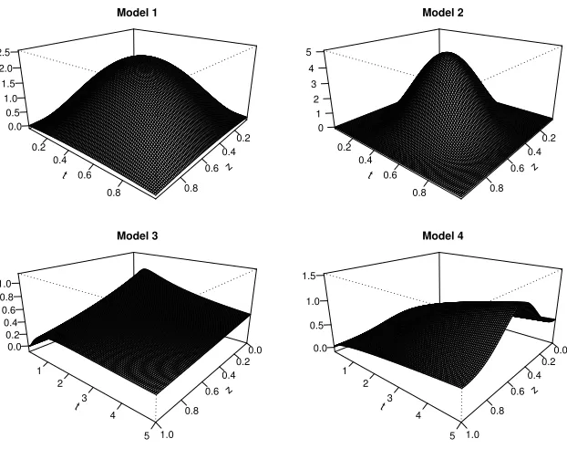
z 0.2 0.4 0.6 0.8 t 0.2 0.4 0.6 0.8 0.0 0.5 1.0 1.5 2.0 2.5 Model 1 z 0.2 0.4 0.6 0.8 t 0.2 0.4 0.6 0.8 0 1 2 3 4 5 Model 2 z 0.0 0.2 0.4 0.6 0.8 1.0 t 1 2 3 4 5 0.0 0.2 0.4 0.6 0.8 1.0 Model 3 z 0.0 0.2 0.4 0.6 0.8 1.0 t 1 2 3 4 5 0.0 0.5 1.0 1.5 Model 4
Figure 1: The true two-dimensional hazards in the simulation study.
The second objective is addressed by comparing the two proposed bandwidth estimates for the local linear estimator with the infeasible bandwidth selectors considered as benchmarks. Such a comparison will give some guidance as to how well the feasible bandwidth selectors are doing.
4.2. Simulation settings
We consider a model with a one-dimensional constant markerZthat takes values in the interval [0, τ]. We consider four two-dimensional hazards. The first two were also considered in Nielsen (1998) and the other two were also considered in Spierdijk (2008). The assumed true hazard rates are:
α1(t,z) = B(t,2,2)×B(z,2,2), t,z∈[0,1]
α2(t,z) = B(t,4,4)×B(z,4,4), t,z∈[0,1]
α3(t,z) = 1
t
ψ(log(t)−z)
Φ(z−log(t)), t∈(0,5],z∈[0,1]
α4(t,z) = 32t1/2exp
−1
2cos(2πz)− 3 2
, t∈(0,5],z∈[0,1]
(7)
whereB(·,a,a) denotes the density of a Beta with shape and scale parameters equal toa, andψ(·) andΦ(·) denote the density and the cumulative distribution function of a Standard Normal, respectively. These four true hazards are shown in Figure 1.
samples of sizen=100,500,1000 and 5000. The explicit algorithms to simulate both types of samples are provided in Appendix B, specifically in subsections Appendix B.2 and Appendix B.3. From these algorithms the data are recorded in a discrete way so that the estimators (local linear and LLLC) can be calculated from the discrete versions provided in subsection Appendix B.1. This simulation strategy is similar to the one considered in Nielsen (1998) and Nielsen and Tanggaard (2001). We discretise the simulated data in a two-dimensional grid into [0, τ]×[0,1] with sizeM×M0andτ =1 for models 1 and 2 andτ =5 for models 3 and 4. To ensure the stability of the results and therefore the validity of the approximation we choose the valuesM=M0=100. Bigger grid sizes do not appear to alter our conclusions.
Finally, the kernel estimators are always calculated using the kernelK(x)=3003/2048(1−x2)6I(−1<x< 1). The bandwidth selectors are calculated as minimisers of the corresponding scores into an equally spaced grid of bandwidths. We define a two-dimensional grid of 100 bandwidths,b=(b0,b1), withb0∈[τ/n, τ/2] andb1 ∈[1/n,0.5] for each model.
The comparison among hazard estimators is made by evaluating the following performance measure:
err(bαK,b)=n−1 M
X
r=1
M0 X
r0=1
bαK,b(xr,r0)−α(xr,r0)
2E
r,r0, (8)
for any estimatorbαK,b with bandwidthb = (b0,b1) and kernelK. This is just the discrete version of the global measure of the estimation error in (4). From each simulated sample, each estimator provides a value of the error (8), and the comparisons are made from the averaged errors over the S simulated samples in each scenario.
4.3. Simulation Results
In this section we go through the obtained results from the simulation experiments under the scenarios defined above and draw some conclusions about the two objectives we pursue.
Each true hazard is estimated using two types of estimators: the local linear (LL) and the LLLC. The comparison between these two estimators is done in two steps. Firstly, by considering the best possible situation, i.e. at their respective best optimal bandwidths (defined and denoted above byeb0andb0). Secondly,
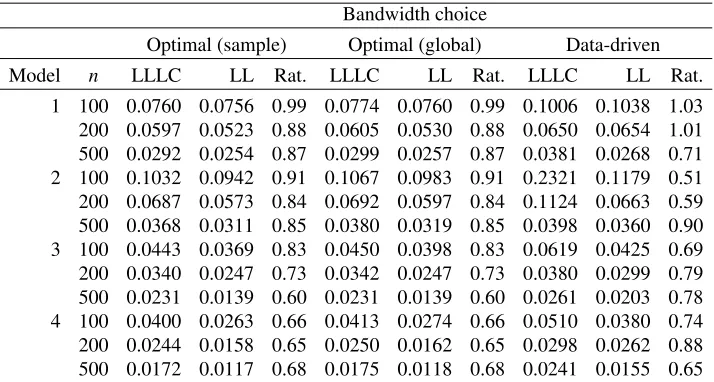
we compare the estimators using data-driven bandwidth selection, which would be the case in practice. The simulation results are shown in Table 1 and Table 2. The numbers in these tables correspond to the averaged (along the S simulated samples) values of the performance measure in (8). The last three columns in the tables correspond to the practical estimators, specifically the LLLC estimator with cross-validated bandwidth (bbCV) and the local linear estimator with do-validated bandwidth (bbDO).
Bandwidth choice
Optimal (sample) Optimal (global) Data-driven
Model n LLLC LL Rat. LLLC LL Rat. LLLC LL Rat.
[image:10.612.128.485.82.273.2]1 100 0.0760 0.0756 0.99 0.0774 0.0760 0.99 0.1006 0.1038 1.03 200 0.0597 0.0523 0.88 0.0605 0.0530 0.88 0.0650 0.0654 1.01 500 0.0292 0.0254 0.87 0.0299 0.0257 0.87 0.0381 0.0268 0.71 2 100 0.1032 0.0942 0.91 0.1067 0.0983 0.91 0.2321 0.1179 0.51 200 0.0687 0.0573 0.84 0.0692 0.0597 0.84 0.1124 0.0663 0.59 500 0.0368 0.0311 0.85 0.0380 0.0319 0.85 0.0398 0.0360 0.90 3 100 0.0443 0.0369 0.83 0.0450 0.0398 0.83 0.0619 0.0425 0.69 200 0.0340 0.0247 0.73 0.0342 0.0247 0.73 0.0380 0.0299 0.79 500 0.0231 0.0139 0.60 0.0231 0.0139 0.60 0.0261 0.0203 0.78 4 100 0.0400 0.0263 0.66 0.0413 0.0274 0.66 0.0510 0.0380 0.74 200 0.0244 0.0158 0.65 0.0250 0.0162 0.65 0.0298 0.0262 0.88 500 0.0172 0.0117 0.68 0.0175 0.0118 0.68 0.0241 0.0155 0.65
Table 1: Comparison between the local linear local constant (LLLC) estimator and the local linear (LL) estimator -case of complete samples. The numbers in the table show the average (along the simulated samples) of the performance measure in (8). Columns 5, 8 and 11 show the ratio between the LL and LLLC errors. Columns 3–5 correspond to the estimators calculated at their best optimal bandwidth at each sample (eb0). Columns 6–8 correspond to the best global optimal bandwidths (b0). Columns 9–11 correspond to the
data-driven bandwidth choice, which is cross-validation for LLLC and do-validation for LL.
Bandwidth choice
Optimal (sample) Optimal (global) Data-driven
Model n LLLC LL Rat. LLLC LL Rat. LLLC LL Rat.
[image:10.612.128.484.372.574.2]1 100 0.0947 0.0870 0.92 0.0965 0.0902 0.92 0.1641 0.0980 0.60 200 0.0569 0.0499 0.88 0.0599 0.0534 0.88 0.0830 0.0578 0.70 500 0.0262 0.0212 0.81 0.0267 0.0216 0.81 0.0478 0.0229 0.48 2 100 0.1280 0.1151 0.90 0.1326 0.1233 0.90 0.2026 0.1530 0.75 200 0.1007 0.0961 0.95 0.1022 0.0997 0.95 0.1262 0.1047 0.83 500 0.0521 0.0488 0.94 0.0530 0.0497 0.94 0.1016 0.0523 0.52 3 100 0.0441 0.0362 0.82 0.0456 0.0374 0.82 0.0538 0.0406 0.75 200 0.0288 0.0193 0.67 0.0289 0.0200 0.67 0.0377 0.0239 0.63 500 0.0181 0.0102 0.56 0.0181 0.0103 0.56 0.0198 0.0147 0.74 4 100 0.0365 0.0311 0.85 0.0380 0.0330 0.85 0.0443 0.0372 0.84 200 0.0304 0.0237 0.78 0.0308 0.0254 0.78 0.0357 0.0283 0.79 500 0.0176 0.0137 0.78 0.0180 0.0138 0.78 0.0245 0.0178 0.73
z 0.2
0.4
0.6
0.8 t
0.2 0.4
0.6
0.8 0
1 2 3 4 5
LLLC / LL (model 1)
z 0.2
0.4
0.6
0.8 t
0.2 0.4
0.6
0.8 0
2 4 6 8 10
LLLC / LL (model 2)
z 0.0 0.2
0.4
0.6
0.8
1.0 t
1 2
3
4
5 1
2 3 4 5
LLLC / LL (model 3)
z 0.0 0.2
0.4
0.6
0.8
1.0 t
1 2
3
4
5 1.0
1.5 2.0
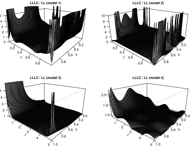
[image:11.612.149.461.64.311.2]LLLC / LL (model 4)
Figure 2: Ratio between the LLLC estimator and the local linear estimator from the 5% best sample for the LLLC estimator (sample sizen=500 and no filtration). The estimators are calculated with their respective best optimal bandwidths.
estimators from one simulated sample (the estimators were calculated using their best possible bandwidths with this sample). The sample we choose for the plots is one of the best for the LLLC estimator. Specifically, we choose the sample corresponding to the 5% quantile of the performance measure, which is calculated by ordering the samples according to the reported error by the estimator, and then choosing the sample that gives the highest error of the 5% simulated samples with the best performance.
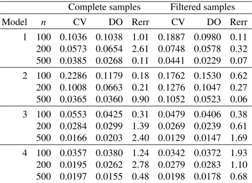
As a next step we asses the performance of the bandwidth selectors considered for the local linear estimator (our second objective). Table 3 shows the results of the performance measure in (8) for each method in each simulated scenario. To gain a clearer insight into the performance of the different methods, we calculate the relative error with respect to the infeasible best possible bandwidth at each sample (eb0). This measure is
defined as
Rerr=averrDO−averr0 averrCV−averr0
, (9)
whereaverr• is the average of the error measure in (8) along the S simulated samples and considering a
specific criterion for the bandwidth selection (CV, DO oreb0). The resulting values for each model and the
Table 3: Comparison between cross-validation and do-validation for the local linear estimator. The numbers in the table consist of the average (along the simulated samples) of the performance measure in (8). Columns 5 and 8 show the relative error defined in (9).
Complete samples Filtered samples
Model n CV DO Rerr CV DO Rerr
1 100 0.1036 0.1038 1.01 0.1887 0.0980 0.11 200 0.0573 0.0654 2.61 0.0748 0.0578 0.32 500 0.0385 0.0268 0.11 0.0441 0.0229 0.07 2 100 0.2286 0.1179 0.18 0.1762 0.1530 0.62 200 0.1008 0.0663 0.21 0.1276 0.1047 0.27 500 0.0365 0.0360 0.90 0.1052 0.0523 0.06 3 100 0.0553 0.0425 0.31 0.0479 0.0406 0.38 200 0.0284 0.0299 1.39 0.0269 0.0239 0.61 500 0.0166 0.0203 2.40 0.0129 0.0147 1.69 4 100 0.0357 0.0380 1.24 0.0342 0.0372 1.93 200 0.0195 0.0262 2.78 0.0279 0.0283 1.10 500 0.0197 0.0155 0.48 0.0198 0.0178 0.68
reported in Table 3 is that do-validation outperforms cross-validation most of the time for both complete and filtered samples.
5. An application to old-age mortality
In this section we provide an illustration of the methods described in this paper to the dataset used by Fledelius et al. (2004), which consists of old-age mortality data of Swedish women. Fledelius et al. (2004) argue that local linear estimation is particularly important in studies of old age mortality because of its su-perior bias properties (compared to local constant estimation). The dataset covers the calendar years 1988 to 1997 and the ages 90 and above. The aim is to estimate the two-dimensional hazard or force of mortal-ity,α(t,z). In our formulation of the hazard function, age is time and calendar year is a one-dimensional covariate. In the study by Fledelius et al. (2004), the estimation was calculated using the same local lin-ear estimator we defined in (3), but with a subjective bandwidth choice. Based on experience, the authors considered a bandwidth parameter for the time dimension ofb0 = 7 andb1 = 4 for the covariate. Here we consider two practical data-driven bandwidth choices, namely the cross-validated and the do-validated bandwidths, which were defined in Section 3. To calculate the estimators, we use the Epanechnikov kernel as the symmetric kernelK, which was also used by Fledelius et al. (2004).
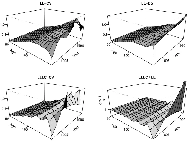
Figure 3 shows the resulting smooth two-dimensional hazard estimates of the force of mortality for ages 90 and above between 1988 and 1997. The top left panel shows the local linear estimator with cross-validated bandwidths, which in this case arebbCV = (5,2). The hazard estimate using the do-validated bandwidths
ofbbDO = (3.75,17.25) is shown in the top right panel. The LLLC estimator is shown below using the
provide surfaces which are increasing with respect to age. However, they exhibit different shapes and rates of increase. The ratio between the LLLC estimator and the LL estimator is plotted in the right bottom panel in Figure 3. As we would expect, the major differences between the estimators arise at the boundary points. We should also point out that cross-validation (for both the local linear and the LLLC estimators) does not work well in this case. The cross-validation score is minimised at unacceptable undersmoothing levels which lead to very noisy estimates.
In order to gain a better insight into the differences among our estimates, we have plotted in Figure 4 the estimated force of mortality for three different years, 1989, 1992, and 1996.
Each panel in Figure 4 shows the three practical estimates that we are comparing, namely the cross-validated and do-validated local linear estimator and the cross-validated LLLC estimator. We have also plotted the local linear estimator with the bandwidth vector used by Fledelius et al. (2004). The mortality curves in this figure, as well as the surfaces in Figure 3, show that there has been a slight decline in female mortality over the decade which is in line with the results of previous studies. However, the time trend exhibited by each estimate is quite different for the ages 105 and above. Clearly, the LLLC estimator fails dramatically in this age range, although the cross-validated local linear estimator in years 1989 and 1992 seems to perform equally bad.
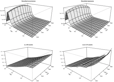
As discussed above, the fact that the estimator is a ratio (see equation 3) leads to problems in areas with very small exposures. The visualisation technique provided in Figure 5 makes it possible to understand when dramatic peaks might be due to the level of exposures approaching zero. In this figure, the top graphs show the smoothed local linear occurrences and exposures (given byO11(·,·) andE11(·,·) in equation (3)). From this we can see that the estimated mortality above 105 years of age is based on almost no information and the visual analysis becomes difficult. Therefore, the estimators should be compared in the area with more exposure, which we do in the lower graphs of Figure 5. This analysis confirms that the do-validated local linear estimator gives a better estimate of the mortality rates than the estimators based on cross-validated bandwidths. In fact, the do-validated LL estimator provides conclusions similar to the ones guided by expert opinion in Fledelius et al. (2004)).
6. Conclusion
Year
1990
1995 Age
90
100 0.5
1.0
LL−CV
Year
1990
1995 Age
90
100 0.5
1.0
LL−Do
Year
1990
1995 Age
90
100 0.5
1.0
LLLC−CV
Year
1990
1995 Age
90
100 Ratio
1 2 3
[image:14.612.148.457.188.424.2]LLLC / LL
Death rates for women in 1990
Age
Death intensity
90 95 100 105
0.2 0.4 0.6 0.8 1.0
1.2 LL−DO
LL−CV LLLC−CV FGNP−2004
Death rates for women in 1992
Age
Death intensity
90 95 100 105
0.2 0.4 0.6 0.8 1.0
1.2 LL−DO
LL−CV LLLC−CV FGNP−2004
Death rates for women in 1996
Age
Death intensity
90 95 100 105
0.2 0.4 0.6 0.8 1.0
1.2 LL−DO
[image:15.612.99.510.171.485.2]LL−CV LLLC−CV FGNP−2004
Year
1988
1990
1992
1994
1996 Age
90
95
100
105 0e+00
1e+10 2e+10 3e+10
Smoothed occurrences
Year 1988
1990
1992
1994
1996 Age
90
95
100
105 0e+00
5e+10 1e+11
Smoothed exposures
Year
1988
1990
1992
1994
1996 Age
90
95
100 0.2
0.4 0.6 0.8 1.0
LL−DO (zoom)
Year
1988
1990
1992
1994
1996 Age
90
95
100 0.2
0.4 0.6 0.8 1.0
[image:16.612.109.498.175.457.2]LLLC−CV (zoom)
and Bagkavos and Patil (2008), transformation methods (see Spreeuw et al. (2013) or multiplicative bias correction methods (see Mammen and Nielsen (2007)) could be useful starting points for further research. It is perhaps surprising that so little focus has been given to provide plots of the fully unrestricted hazard estimator given the enormous popularity of structured hazard models. While structured models, like the popular Cox model, might summarise data in a convenient way, it is also true that important details of the overall hazard might be missed when imposing structure. Therefore, the unrestricted hazard considered in this paper should be recommended as an important part of the applied statisticians tool box when working with survival data.
Acknowledgements
The authors thank the Centro de Servicios de Inform´atica y Redes de Comunicaciones (CSIRC), Universidad de Granada, for providing the computing time (all the calculations have been done in R –R Development Core Team, 2011). We also thank Prof. Guill´en (University of Barcelona, Spain) for providing us with the mortality dataset. This work has been financially supported by the Spanish “Ministerio de Ciencia e Innovaci´on” by the grant MTM2008-03010,“Junta de Andaluc´ıa” grant TIC-06902 and the European Com-mission under the Marie Curie Intra-European Fellowship FP7-PEOPLE-2011-IEF Project number 302600. Finally the authors would like to thank the anonymous reviewers for their valuable comments and sugges-tions to improve the quality of the paper.
References
Aalen, O.O. (1978), Non-parametric inference for a family of counting processes.Annals of Statistics, 6, 701–726.
Andersen, P., Borgan, O., Gill, R. and Keiding, N. (1993),Statistical Models Based on Counting Processes. Springer, New York.
Andersen, P.K. and Gill, R.D. (1982), Cox’s Regression Model for Counting Processes: A Large Sample Study.Annals of Statistics, 10(4), 1100–1120.
Bagkavos, D. (2011), Local linear hazard rate estimation and bandwidth selection.Annals of the Institute of Statistical Mathematics, 63, 1019–1046.
Bagkavos, D. and Patil, P.N. (2008), Local polynomial fitting in failure rate estimation.IEEE Transactions on Reliability, 57 (1),41–52.
Buch-Kromann, T. and Nielsen, J.P. (2012), Multivariate density estimation using dimension reducing in-formation and tail flattening transin-formations for truncated or censored data.Annals of the Institute of Statistical Mathematics, 64(1), 167–192.
Fledelius, P., Guill´en, M., Nielsen, J.P. and Petersen, K.S. (2004), A Comparative Study of Parametric and Nonparametric Estimators of Old-Age Mortality in Sweden.Journal of Actuarial Practice2004(1), 101– 126.
Fleming, T.R. and Harrington, D.P. (1991),Counting Processes and Survival Analysis. Wiley, New York.
G´amiz, M.L., Mart´ınez-Miranda, M.D. and Nielsen, J.P. (2013), Smoothing survival densities in practice.
Computational Statistics and Data Analysis, 58, 368–382.
Jones, C. (1993) Simple boundary correction for kernel density estimation.Statistics and Computing, 3, 135–146.
Kim, C., Oh, M., Yang, S.J. and Choi, H. (2010), A local linear estimation of conditional hazard function in censored data.Journal of the Korean Statistical Society, 39, 347–355.
Mammen, E., Mart´ınez-Miranda, M.D., Nielsen, J.P. and Sperlich, S. (2011), Do-validation for kernel den-sity estimation.Journal of the American Statistical Association, 106, 651–660.
Mammen, E. and Nielsen, J.P. (2007), A general approach to the predictability issue in survival analysis with applications,Biometrika, 94(4), 873–892.
Mart´ınez-Miranda, M.D., Nielsen, J.P. and Sperlich, S. (2009), One sided cross-validation for density esti-mation with an application to operational risk. In: G.N. Gregoriou (eds.)Operational Risk Towards Basel III: Best Practices and Issues in Modelling. Management and Regulation, 177–195. John Wiley and Sons, New Jersey.
Martinussen, T. and Scheike, T.H. (2009), The additive hazards model with high-dimensional regressors.
Lifetime Data Analysis, 15, 330–342.
Nielsen, J.P. (2003), Variable bandwidth kernel hazard estimators,Journal of Nonparametric Statistics3, 355–376.
Nielsen, J.P. and Linton, O.(1995), Kernel estimation in a non-parametric marker dependent hazard model.
Annals of Statistics, 23, 1735–1748.
Nielsen, J.P. (1998), Marker dependent kernel estimation from local linear estimation.Scandinavian Actu-arial Journal, 2, 113–224.
Nielsen, J.P. and Tanggaard, C. (2001), Boundary and bias correction in kernel hazard estimation. Scandi-navian Journal of Statistics, 28, 675–698.
S´anchez-Sellero, C., Gonz´alez-Manteiga, W. and Cao, R. (1999), Bandwidth selection for kernel density estimation with truncated and censored data.Annals of the Institute of Statistical Mathematics, 51(1), 51–70.
Savchuk, O.Y., Hart, J.D. and Sheather, S. (2010), Indirect cross-validation for Density Estimation.Journal of the American Statistical Association, 105, 415–423.
Spierdijk, L. (2008), Nonparametric conditional hazard rate estimation: A local linear approach. Computa-tional Statistics and Data Analysis,52, 2419–2434.
Spreeuw, J., Nielsen, J.P. and Jarner, S.F. (2013) A visual test of mixed hazard models, SORT-Statistics and Operations Research Transactions, in press.
Appendix A. Asymptotic properties of the local linear hazard estimator
The asymptotic properties ofbαK,bare derived in Nielsen (1998) and are established as follows: Letϕ(x)=
ft(z)y(t) andϕ(x)>0, additionally we assume the following regularity conditions:
(i) The hazard function,αandϕare fourth and twice continuously differentiable atx, respectively. (ii) The kernelKhas bounded support, is symmetric around zero and is continuous.
(iii) Suppose thatn|b| → ∞andb→0, where|b|=Qd
j=0bj.
(iv) There exist a functionγ ∈C1([0, τ]) positive intwhich is the limit of the exposure function that is sups∈[0,τ]
Y
(n)(s)/n−γ(s)
P
−→0. Moreover sups∈[0,τ]
nE
n
I(Y(n)(s))/Y(n)(s)o−1− {γ(s)}−1
−→0.
Let the kernel moments be defined as:κ1j=
R
Rd+1υ
2
jK(υ)dυ, for j=0, . . . ,d, andκ2=
R
Rd+1K(υ)
2dυ.
Then the pointwise asymptotic distribution ofbαK,b(x) is analysed by splitting the errorbαK,b(x)−α(x) into
the variable part and a stable part, which leads to the following
(n|b|)1/2{bαK,b(x)−α(x)−Bx}
D
−→ N(0, σ2x)
where
Bx= d
X
j=0
κ1jb2j
1 2
∂2α(x)
∂x2
j +o d X
j=0
b2j
, and σ2
x=κ2
α(x)
ϕ(x)
The required symmetry for the kernelK in assumption (ii) is not essential in developing these asymptotics; however, it allows for simpler expressions. In fact, in the limit the stochastic local linear kernelKx,b(u) sim-ply becomes the deterministicK(u)/ϕ(x). For asymmetric kernels these asymptotic results hold in exactly the same way apart from the involved kernel constantsκ2 andκ1j, j =0,1, . . . ,d. Specifically, these
con-stants take on the values ¯κ2=
R
[K∗(u)]2duand ¯κ1j=
R
u2
jK
kernelK∗(u) which is rather more complicated. For the particular case thatd=1 this equivalent kernel can
be written as
K∗(u0,u1)= 1
ϕ(x)
µ2(K)+µ1(K)2−µ1(K)(u0+u1)
µ2(K)−µ1(K)2
K(u0)K(u1),
whereµ1(K)=
R
vK(v)dvandµ2(K)=
R
v2K(v)dv. For higherdthe expression of the equivalent kernel can also be derived, but this would require some more calculations.
The martingale nature of the problem transfers weak convergence intoL2–convergence (see Andersen et al. (1993)), when we assume that the second condition in assumption (iv) holds. Thus we get that
EhbαK,b(x)−α(x)
i2
=B2x+(n|b|)1/2Vx+o
d X
j=0
b4j+(n|b|)1/2
.
Applying Fubini’s Theorem therefore leads to the following asymptotic expansion of the Mean Integrated Square Errors (MISEs)
MIS EbαK,b(x)
= Pd
j=0κ1jb2j
R1
0
1 2
∂2α(x)
∂x2
j 2
dx
+(n|b|)−1κ 2
R1 0
α(x)
ϕ(x)dx+o
Pd
j=0b4j+(n|b|)
1/2,
(A.1)
involving the symmetric multiplicative kernelK, whereκ2andκ1j,j=0, . . . ,dare defined above. Similarly,
we can write the expression forMIS EbαKA,b(x)
for the case of asymmetric KA analogously to (A.1) by
replacingκ2andκ1jwith ¯κ2and ¯κ1jfor j=0, . . . ,d.
The above MISE calculations are required to develop the do-validation method of Mammen et al. (2011). The key is to find the correct rescaling constantCthat allows us to transform the MISE optimal bandwidth for the local linear estimator using asymmetric kernelsKAto be a MISE optimal bandwidth for the estimator using the kernel with symmetric componentsK. In the paper by Mammen et al. (2011) this constantCwas derived by first obtaining closed-form expressions for the MISE-optimal bandwidths for each local linear estimator. However, such closed-form expressions are not available for dimensionsd>1 unless we assume that the vector of bandwidths is determined by a single scalarb>0. Instead we start by assuming a simpler situation to get the MISE-optimal bandwidths and calculateCand later we prove that in the general case of
b=(b0, . . . ,bd) thisCremains exactly the same. Forb =b×(1, . . . ,1) withb>0, the MISE-optimalbis
given by:
bMIS E=
κ2 κ2 1 R
α(x){ϕ(x)}−1dx
Pd
j=0
R
(∂2∂α(x)
x2
j
)2dx
1/(d+5)
n−1/(d+5), (A.2)
where we assume a symmetric multiplicative kernel with equal componentsKj = Kfor all j = 0, . . . ,d.
Similarly, the MISE-optimal bandwidth for the estimatorbαKA, involving the asymmetric kernelKA, is given
by:
bAMIS E=
¯ κ2 ¯ κ2 1 R
α(x){ϕ(x)}−1dx
Pd
j=0
R
(∂2∂αx(2x)
j
)2dx
1/(d+5)
Therefore the rescaling constantCwhich is defined as the ratio between (A.2) and (A.3) becomes:
C=
κ2/κ12 ¯
κ2/κ¯12
1/(d+5)
. (A.4)
Now we assume the general case ofb=(b0, . . . ,bd) but with the restriction thatKj=Kfor all j=0, . . . ,d.
LetbAMIS Edenote the MISE-optimal bandwidth for the estimatorbαKA. Through some simple calculations we
can prove that the rescaledCbAMIS EwithC=
κ
2/κ21
¯
κ2/κ¯21
1/(d+5)
is optimal in the MISE sense for the estimatorbαK.
We can therefore conclude that for any consistent estimatorbb
A
of the optimalbAMIS E, the rescaled version
Cbb
A
will be a consistent estimator of the optimalbMIS Efor the preferred hazard estimatorbαK.
Appendix B. Simulation and approximation strategies
The purpose of this section is to derive the discrete version of the hazard estimator and the corresponding scores defined for bandwidth selection purposes in the the paper. These expressions are necessary to deal with data applications such as mortality studies, where the data are given as occurrences and exposures for discrete points. These occurrences and exposures are just discretised versions of the counting processes
NiandYi, defined in Subsection 2. Deriving an expression of the estimator from discretised variables is a
simple exercise that we will carry out in Subsection Appendix B.1.
Apart from being required to deal with data applications, the discrete versions are useful for computational purposes in simulation studies. Instead of simulating the continuous scenario formulated in the model di-rectly, it is much faster and more convenient to simulate the data on a lower level of aggregation and then to implement the methods using the discrete versions. Specific algorithms to simulate this kind of data are provided in Subsections Appendix B.2 and Appendix B.3. Note that this strategy in practice is justified as a numerical approximation of the integrals involved in the estimators. Thus, the level of aggregation should be low enough to provide stable approximations. In the simulation experiments described in Section 4 we used a grid of 100 two dimensional points, which was enough to guarantee the stability of the results.
Appendix B.1. Discrete approximations of the hazard estimators and the bandwidth selection strategies
In the continuous scenario we assume that we observenindividuals and have observations of type{(N1,Z1,Y1),
. . . ,(Nn,Zn,Yn)}which are independent and identically distributed. In a practical scenario such detailed data
may be provided in an aggregated way. To simplify the derivations presented here we assume that the marker
Zis unidimensional (d=1). Let us assume a practical situation where we only have observations atM <n
discrete time points,t1, . . . ,tM, and M0 < n discrete values of the covariate, Z1, . . . ,ZM0. Then for each
r0=1, . . . ,M0we have a sample path{(N
r0,1,Yr0,1, . . . ,(Nr0,n
r0,Yr0,n
r0)}of the counting process with intensity
processλk(t,Zr0)=α(t,Zr0)Yr0,l(t),l=1, . . . ,nr0andPM 0
at any estimation pointx=(t,z)tgiven in (3) can be approximated as follows:
bαK,b(x)=
M0 X
r0=1
nr0 X
l=1
M
X
r=1
Z tr
tr−1
[1−(x−xr,r0)tD(x)−1c1(x)]Kb
0(t−s)Kb1(z−Zr0)dNr0,l(s)
M0 X
r0=1
nr0 X
l=1
M
X
r=1
Z tr
tr−1
[1−(x−xr,r0)tD(x)−1c1(x)]Kb
0(t−s)Kb1(z−Zr0)Yr0,l(s)ds
≈
M0 X
r0=1
M
X
r=1
[1−(x−xr,r0)tD(x)−1c1(x)]Kb
0(t−t
∗
r)Kb1(z−Zr0)
nr0 X
l=1
Z tr
tr−1
dNr0,l(s)
M0 X
r0=1
M
X
r=1
[1−(x−xr,r0)tD(x)−1c1(x)]Kb
0(t−t
∗
r)Kb1(z−Zr0)
nr0 X
l=1
Z tr
tr−1
Yr0,l(s)ds
withxr,r0 = (tr,zr0) andt∗
r = (tr−1+tr)/2, for r = 1, . . . ,M andr0 = 1, . . . ,M0. Here the bandwidth is
b=(b0,b1)tand we assume the same kernelKfor both the marker and time. From the expression above we can identify the occurrences and the exposures as follows:
Or,r0=
nr0 X
j=1
Z tr
tr−1
dNr0,j(s),
and
Er,r0=
nr0 X
j=1
Z tr
tr−1
Yr0,j(s)ds,
for r = 1, . . . ,M andr0 = 1, . . . ,M0. Note thatO
r,r0 represents the observed occurrences of the
count-ing processes{Nr0,1, . . . ,Nr0,n
r0}, and Er,r0 represents the observed exposures from the counting processes {Yr0,1, . . . ,Yr0,n
r0}in the interval [tr−1,tr) (forr=1, . . . ,Mandr
0 =1, . . . ,M0). Thus, from a common
dis-crete dataset consisting of{(xr,r0 =(tr,zr0),Er,r0,Or,r0);r =1, . . . ,M,r0=1, . . . ,M0}, the local linear hazard
estimator can be calculated from the following discrete approximation:
e αK,b(x)=
M0 X
r0=1
M
X
r=1
{1−(x−xr,r0)tDe(x)−1
ec1(x)}Kb0(t−t
∗
r)Kb1(z−Zr0)Or,r0
M0 X
r0=1
M
X
r=1
{1−(x−xr,r0)tDe(x)−1
ec1(x)}Kb0(t−t
∗
r)Kb1(z−Zr0)Er,r0
whereec1(x)=(ec1,0(x),ec1,1(x))
tand
e
D(x)=(dej,k(x))j,k(j,k=0,1) are approximations of the momentsc1(x) andD(x) in (3), which are given by:
ec1,0(x) =
M
X
r=1
M0 X
r0=1
Kb0(t−t
∗
r)Kb1(z−zr0)(t−t
∗
r)Er,r0
ec1,1(x) =
M
X
r=1
M0 X
r0=1
Kb0(t−t
∗
r)Kb1(z−zr0)(z−zr0)Er,r0
e
d0,0(x) =
M
X
r=1
M0 X
r0=1
Kb0(t−t
∗
r)Kb1(z−zr0)(t−t
∗
r)
2E
r,r0
e
d0,1(x) =
M
X
r=1
M0 X
r0=1
Kb0(t−t
∗
r)Kb1(z−zr0)(t−t
∗
r)(z−zr0)Er,r0
e
d1,1(x) =
M
X
r=1
M0 X
r0=1
Kb0(t−t
∗
r)Kb1(z−zr0)(z−zr0)
2E
r,r0.
Using similar arguments one can define discrete versions of the performance measure in (4) and the cross-validation score as follows:
Q0(b)≈n−1
M
X
r=1
M0 X
r0=1 h
eαK,b(xr,r0)−α(xr,r0) i2
Er,r0, (B.2)
and
b
Q0(b)≈
M
X
r=1
M0 X
r0=1
e αK,b(xr,r0)
2
Er,r0−2
M
X
r=1
M0 X
r0=1 e α[r,r0]
K,b (xr,r0)Or,r0, (B.3)
whereeα[Kr,,rb0]is the (discrete) hazard estimator arising when the dataset is changed by settingOr,r0=Or,r0−1.
Appendix B.2. Simulating complete samples
Here we describe an algorithm to simulate complete samples from the models defined in (7). As we indi-cated above, the data are obtained in an aggregated way so that each simulated sample will be a set such that{(xr,r0=(tr,zr0),Er,r0,Or,r0);r=1, . . . ,M,r0=1, . . . ,M0}. The models are defined withZbeing a
unidi-mensional marker with range (0,1) and time is defined in [0,1] for models 1 and 2 and in (0,5] for the two last models. Let us now consider the time interval [0, τ]. The algorithm to simulate a complete (not filtered) sample can be described as follows:
Algorithm.
Step 1. Define the grid points{tr :r =1, . . . ,M}and{zr0 : r0 =1, . . . ,M0}as regular sequences between
[0, τ] and [0,1], respectively. LetδMbe the step length of the time sequence i.e.δM=t2−t1.
Step 3. For each marker value in the gridzr0,r0=1, . . . ,M0, the occurrences and the exposures,{Or,r0,Er,r0;r=
1, . . . ,m}, are derived as follows:
(i) Calculate the number of individuals at risk at the initial timet1by counting the number of simu-latedZifalling into [zr0−1,zr0). Letnr0denote the total number of observations for eachr0(clearly PM0
r0=1nr0 =n). Using the notation from subsection Appendix B.1 the discretised risk processes
satisfy:Y(nr0)
r0 (t1) :=Pnr
0
l=1Yr0,l(t1)=nr0.
(ii) Generate the number of failures or occurrences at the initial timet1, which is denoted byO1,r0.
This is done by simulating from a Binomial with sizeY(nr0)
r0 (t1) and probabilityα(t1,zr0)δM.
(iii) Calculate the size of the risk set,Y(nr0)
r0 (tr), and generate the occurrences,Or,r0, at the rest of the
time points in the gridtr(r=2, . . . ,M) by the following recursive expressions:
Y(nr0)
r0 (tr) = Y
(nr0)
r0 (tr−1)−Or−1,r0,
Or,r0 ,→ B
Y(nr0)
r0 (tr), α(tr,zr0)δM
.
(iv) Finally, the exposuresEr,r0is calculated asEr,r0=Y(nr 0)
r0 (tr)δM.
Step 4. Repeat Step 3 for eachr0=1, . . . ,M0to get the sample{(x
r,r0 =(tr,zr0),Er,r0,Or,r0);r=1, . . . ,M,r0=
1, . . . ,M0}.
Appendix B.3. Simulating left truncation and right censoring
We will now introduce truncation and censoring following a similar method as Buch-Kromann and Nielsen (2012). For the models 1 to 4 in (7), the number of censored observations was generated from a Binomial distribution with success probability pcens =0.01. This corresponds to an overall proportion of right
cen-soring of about 20% with a grid size ofM =100 time points. The proportion of left truncated observations in the sample was ptrun =0.25. The algorithm to simulate one sample with these levels of censoring and
truncation follows a similar structure to the algorithm in subsection Appendix B.2. The difference is just in Step 3, which now runs as follows:
Step 3. For each marker value in the gridzr0,r0=1, . . . ,M0the occurrences and exposures,{Or,r0,Er,r0;r=
1, . . . ,m}, are derived as follows:
(i) Calculate the number of simulatedZiwhich fall into [zr0−1,zr0) and let this number be denoted
by nr0 (PM 0
r0=1nr0 = n). Calculate the number of individuals at risk at the initial time t1 as:
Y(nr0)
r0 (t1)=nr0(1−ptrun) := enr0.
(ii) Generateenr0 random values{T1,r0, . . . ,T
e
nr0,r0}from a Uniform in [0, τ/2]. Calculate the number
of truncated observations that enter the sample at each timetr(r =1, . . . ,M) by counting the
number of simulatedT·,r0 (r=1, . . . ,M) which fall into [tr−1,tr). LetTr,r0 denote the resulting
counts and update the number of individuals at risk at the initial timet1by calculatingY (nr0)
r0 (t1)=
Y(nr0)
(iii) Generate the number of failures or occurrences at the initial timet1, which is denoted byO1,r0.
This is done by simulating from a binomial with sizeY(nr0)
r0 (t1) and probabilityα(t1,zr0)δM.
(iv) Generate the censoring level at timet1from a binomial with sizeY (nr0)
r0 (t1)−O1,r0and probability
pcens. Let the the generated value be denoted byC1,r0
(v) Calculate the size of the risk set (Y(nr0)
r0 (tr)) and generate the occurrences (Or,r0) and the censoring
levels (Cr,r0) at the rest of time points in the gridtr (r = 2, . . . ,M) by the following recursive
expressions:
Y(nr0)
r0 (tr) = Y(nr
0)
r0 (tr−1)−Or−1,r0+Cr−1,r0−Tr−1,r0,
Or,r0 ,→ B
Y(nr0)
r0 (tr), α(tr,zr0)δM
,
Cr,r0 ,→ B
Y(nr0)
r0 (tr−1)−Or−1,r0,pcens
.
(vi) Finally, the exposureEr,r0is calculated asEr,r0 =Y(nr0)