Numer. Math.
DOI 10.1007/s00211-016-0808-z
Numerische
Mathematik
Edge-based nonlinear diffusion for finite element
approximations of convection–diffusion equations
and its relation to algebraic flux-correction schemes
Gabriel R. Barrenechea1 · Erik Burman2 · Fotini Karakatsani3
Received: 23 September 2015 / Revised: 7 March 2016
© The Author(s) 2016. This article is published with open access at Springerlink.com
Abstract For the case of approximation of convection–diffusion equations using piecewise affine continuous finite elements a new edge-based nonlinear diffusion operator is proposed that makes the scheme satisfy a discrete maximum principle. The diffusion operator is shown to be Lipschitz continuous and linearity preserving. Using these properties we provide a full stability and error analysis, which, in the diffu-sion dominated regime, shows existence, uniqueness and optimal convergence. Then the algebraic flux correction method is recalled and we show that the present method can be interpreted as an algebraic flux correction method for a particular definition of the flux limiters. The performance of the method is illustrated on some numerical test cases in two space dimensions.
Mathematics Subject Classification 65N30·65N12
1 Introduction
For an open bounded polygonal (polyhedral) domain ⊆ Rd,d = 2,3, with
Lipschitz boundary, we consider in this work the steady-state convection–diffusion– reaction equation
B
Gabriel R. Barrenechea [email protected]1 Department of Mathematics and Statistics, University of Strathclyde, 26 Richmond Street, Glasgow G1 1XH, UK
2 Department of Mathematics, University College London, Gower Street, London WC1E 6BY, UK 3 Department of Mathematics, University of Chester, Thornton Science Park,
−ε u+b· ∇u+σ u = f in,
u =g on∂, (1.1)
whereε >0 is the diffusion coefficient,b∈L∞()2is a solenoidal convective field,
σ >0 is a real constant, and f ∈ L2(),g ∈ H12(∂), are given data. In this work
we adopt the standard notation for Sobolev spaces. In particular, for D ⊂ Rd we
denote(·,·)DtheL2(D)[orL2(D)d] inner product, and by · l,D(| · |l,D) the norm
(seminorm) inHl(D)[with the usual convention that H0(D)=L2(D)].
The weak form of problem (1.1) is: Findu ∈H1()such thatu=gon∂and
a(u, v)=(f, v) ∀v∈H01(), (1.2)
where the bilinear formais given by
a(u, v):=ε (∇u,∇v)+(b· ∇u, v)+σ(u, v).
The weak problem (1.2) has a unique solutionu∈ H1()and its solution satisfies
the following maximum principle (see [10]).
Definition 1 (Maximum principle) Assume that f ≥ 0,g ≥ 0 (resp.≤ 0) and the
solutionu of (1.2) is smooth enough. Then, ifσ =0 anduattains a strict minimum
(resp. maximum) at an interior pointx˜ ∈ , thenu is constant in. Ifσ >0, then
the same conclusion remains valid if we suppose in addition that u(˜x) < 0 [resp.
u(x˜) >0].
This work deals with the development of a method that satisfies the discrete analogue of the last definition. The quest for such a method has been a constant for the last couple of decades. Several methods have been proposed over the years, both in the
finite element and finite volume contexts (see [21] for a review). Overall, the common
point of all discretisations that satisfy a discrete maximum principle (DMP) is that they add some diffusion to the equations. This extra diffusion can lead to a linear method, but it is a well-known fact that such a method will provide very diffused numerical solutions, which will converge suboptimally. Due to the previous fact, several methods that add nonlinear diffusion have been proposed.
One approach has been to add a so-called shock-capturing term to the finite element formulation. This typically amounts to a nonlinear diffusion term where the diffusion coefficient depends nonlinearly on the finite element residual, making it large in the zones where the solution is underresolved, but vanish in smooth regions. An analy-sis showing that nonlinear shock capturing methods may lead to a DMP was first
proposed in [5], and then developed further for the Laplace operator in [6], and for
the convection–diffusion equation in [7]. For a review of shock capturing methods,
designed to reduce spurious oscillations, without necessarily satisfying a DMP, see
[14]. More recent nonlinear discretisations, these ones based on the idea of blending
in order to satisfy the DMP, are the works [1,9], where the emphasis has been given to
function). Because of this the analysis of such methods is incomplete even when linear model problems with constant coefficients are considered. In particular, in most cases uniqueness of solutions can not be proved, and the convergence theory is incomplete. On the other hand, driven initially by the design of explicit time stepping schemes for compressible flows, so called flux corrected transport (FCT) schemes and the
related algebraic flux correction (AFC) schemes were introduced [15,19,20]. These
schemes act on the algebraic level by first modifying the system matrix so that it has suitable properties to make the system monotonous, while perturbing the method as little as possible. In the most elementary case the system matrix is simply perturbed to make it an M-matrix, resulting in a linear method. This crude strategy, however, necessarily results in a first order scheme. Then, AFC schemes introduce a nonlinear switch, or flux limiter, thus making the low order monotone scheme active only in the zones where the DMP may be violated. These schemes have also resisted mathematical
analysis for a long time, but a number of results have been proved recently in [2,3].
Indeed, in these references, existence of solutions and positivity have been proved, and a first error analysis has been performed. Nevertheless, it was shown that the DMP, and even the convergence of the discrete solution to the continuous one, depend on the geometry of the mesh.
Another approach to combine monotone (low order) finite element methods with linear diffusion and high order FEM using flux-limiters was proposed very recently
in [13]. It then appears that a cross pollination between the idea of AFC and
shock-capturing could be fruitful.
The objective of the present paper is to further bridge the gap between the shock capturing approach and the algebraic flux correction. Indeed we will consider a
gen-eralisation of the shock-capturing term first introduced in [4] to several dimensions,
using an anisotropic diffusion operator along element edges similar to that introduced
in [7]. We show that the resulting scheme satisfies the DMP and give an analysis of the
method. In particular we show that the new shock capturing term is Lipschitz continu-ous, and, if the mesh is sufficiently regular, linearity preserving (see Sect.2.1), which
allows us to improve greatly on previous results. In Sect.2.2we prove existence of
solutions, the discrete maximum principle, and noticeably, uniqueness in the diffusion dominated regime. We then show error estimates, which, thanks to the combined use of linearity preservation and Lipschitz continuity, turn out to be optimal in the diffusion
dominated regime, for a special class of meshes (see Sect.3). In Sect.4, we revisit
the design principles of AFC and show that the proposed shock-capturing term can be interpreted as an AFC scheme using a special flux, allowing both for a DMP and
Lipschitz continuity. Some numerical results are finally shown in Sect.5.
1.1 Notations
We now introduce some notation that will be needed for the discrete setting. We consider a family{Th}h>0of shape-regular triangulations ofconsisting of disjoint
d-simplicesK. We definehK :=diam(K), andh=max{hK :K ∈Th}. We associate
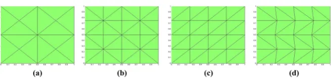
Fig. 1 In two dimensions, meshes (a–c) are examples of symmetric meshes. Mesh (d) is a non-symmetric, non-Delaunay mesh
Vh:= {χ ∈H1():χ|K ∈P1(K)∀K ∈Th}, and Vh0:=Vh∩H01(), (1.3)
whereP(D)is the space of polynomials of degree at mostonD.The nodes ofTh
are denoted by{xi}iN=1, and the usual associated basis functions ofVhare denoted by
{ψi}Ni=1.
We letEhbe the set of the interior edges ofTh. For every edgeE ∈Eh, we define
hE := |E|andωE := {K ∈Th: K∩E = ∅}, and fix one unit tangent vector, denoted
byt.
For an interior nodexi, we define the associated edgesEi := {E ∈ Eh: xi ∈ E}
and the subset ofRd defined by the union of all elements K sharing the nodexi,
i := {x∈ ¯: ∃K ∈Th:x ∈K andxi ∈K}, and the set
Si := {j ∈ {1, . . . ,N}\{i}: xj shares an internal edge withxi}. (1.4)
Finally, we will say that the triangulationThissymmetric with respect to its internal
nodesif for every internal nodexithe following holds: for allj ∈Sithere existsk∈Si
such thatxj−xi = −(xk−xi)(see Fig.1for examples in two space dimensions).
2 The nonlinear discretisation
The standard finite element method for the problem (1.2) takes the form: finduh∈Vh
such thatuh−ubh∈Vh0and
a(uh, vh)=(f, vh) ∀vh ∈Vh0. (2.1)
Here,ubh ∈ Vh is introduced to approximate the boundary conditiong. Then, we
propose the following stabilised method to discretise (1.2): finduh ∈ Vh such that
uh−ubh∈Vh0and
ah(uh;vh):=a(uh, vh)+dh(uh;uh, vh)=(f, vh) ∀vh∈Vh0. (2.2)
The stabilisation termdh(· ; ·, ·)is defined by
dh(wh;uh, vh)=
E∈Eh
[image:4.439.57.385.52.131.2]Here,γ0 > 0, andαE:Vh → [0,1]is defined as follows. First, forwh ∈ Vh, we
defineξwh as the unique element inV
0
hwhose nodal values are given by
ξwh(xi):=
⎧ ⎨ ⎩
j∈Siwh(xi)−wh(xj)
j∈Si|wh(xi)−wh(xj)|, if
j∈Si|wh(xi)−wh(xj)| =0,
0, otherwise.
(2.4)
Then, on eachE,αE is defined by
αE(wh):=max x∈E ξwh(x)
p
, p∈ [1,+∞). (2.5)
The value for pwill determine the rate of decay of the numerical diffusion with the
distance to the critical points. A value closer to 1 will add more diffusion in the far field, while a larger value will make the diffusion vanish faster, but on the other hand,
increasingpmay make the nonlinear system more difficult to solve. In principle, asp
goes to infinity the method will add the perturbations only in points with local extrema.
In our calculations we have tested several different values for p, and have presented
those forp=1,4,8, and 10. The higher values provide better numerical results, while
keeping the nonlinear solver converging within a reasonable number of iterations. In
Sect.5below we present a more detailed study of the behavior of the nonlinear solver
with respect to the value of p.We finally stress the fact that, for any value of p, the
functionαE(wh)is equal to 1 ifwhhas a local extremum in one of the end points of
the edgeE. This property is of fundamental importance for the proof of the discrete
maximum principle below.
2.1 Properties ofdh(·; ·,·)
We start noticing that
j∈Si
|wh(xi)−wh(xj)| =0⇒wh|i =c∈R.
This prevents the method from adding artificial diffusion to the equations in regions in which the solution is constant. Moreover, the method is as well linearity preserving
if the mesh is symmetric with respect to its interior nodes. In fact, if E ∈ Eh has
endpointsxi andxj, andvh∈P1(ωE), then
l∈Si
vh(xi)−vh(xl)=0 and
l∈Sj
vh(xj)−vh(xl)=0, (2.6)
which givesαE(vh)= 0. Then, the method does not add extra diffusion in smooth
regions, whenever the mesh is sufficiently structured. We now state this in a more
pre-cise way. Let us decompose the stabilisation termdhas the sum of edge contributions
dh(uh;vh,zh) =
E∈Eh
dE(uh;vh,zh)
withdE(uh;vh,zh):=γ0h
d
EαE(uh)(∂tvh, ∂tzh)E.
Then, if the mesh is symmetric with respect to its internal nodes andE∈Eh, whenever
vh ∈P1(ωE), the edge diffusion vanishes, this is
dE(vh;wh,zh)=0 ∀wh,zh∈Vh.
As a consequence, if, for a given nodexi, with associated basis functionψi, we denote
the extended macro element˜i := ∪E∈EiωE, then
dh(vh;wh, ψi)=0, ∀wh∈Vh and ∀vh:vh|˜i ∈P1(˜i).
The next step is to show thatdh(·; ·,·)is continuous. More precisely, it is Lipschitz
continuous, and the next result is the first step towards this.
Lemma 1 For anyvh, wh ∈Vh, and any given internal node xi, the following holds
|ξvh(xi)−ξwh(xi)| ≤4
E∈EihE|∂t(vh−wh)|
E∈Ei hE(|∂tvh| + |∂twh|).
(2.7)
Proof It is enough to suppose thatj∈Si|vh(xi)−vh(xj)|>0 and
j∈Si |wh(xi)− wh(xj)|>0, otherwise the claim is obvious. A quick calculation gives
|ξvh(xi)−ξwh(xi)|
=
j∈Sivh(xi)−vh(xj)
E∈EihE|∂tvh| −
j∈Siwh(xi)−wh(xj)
E∈EihE|∂twh| ≤
j∈Si vh(xi)−vh(xj)
−j∈Siwh(xi)−wh(xj)
E∈Ei hE|∂tvh|
+ j∈Si
wh(xi)−wh(xj) 1
E∈EihE|∂tvh|−
1
E∈EihE|∂twh|
≤
E∈EihE|∂t(vh−wh)|
E∈EihE|∂tvh|
+
j∈Siwh(xi)−wh(xj)
E∈EihE(|∂twh| − |∂tvh|)
E∈Ei hE|∂tvh|
E∈Ei hE|∂twh|
≤2
E∈EihE|∂t(vh−wh)|
The following estimate can be proved in an analogous way
|ξvh(xi)−ξwh(xi)| ≤2
E∈EihE|∂t(vh−wh)|
E∈EihE|∂twh| .
Then,
|ξvh(xi)−ξwh(xi)|
≤2 min
1
E∈Ei hE|∂tvh|,
1
E∈EihE|∂twh|
E∈Ei
hE|∂t(vh−wh)|, (2.8)
which gives the desired result upon applying the estimate min{a−1,b−1} ≤ a+2b, for
two positive numbersaandb.
The Lipschitz continuity ofdh(·; ·,·)appears then as a consequence of the previous
result.
Lemma 2 The nonlinear form dh(·; ·,·)is Lipschitz continuous. More precisely, there
exists Clip > 0, independent of h, such that, for allvh, wh,zh ∈ Vh, the following
holds
|dh(vh;vh,zh)−dh(wh;wh,zh)| ≤Clipγ0h|vh−wh|1,|zh|1,. (2.9)
Proof We have
dh(vh;vh,zh)−dh(wh;wh,zh)
=
E∈Eh
γ0hdEαE(vh)∂tvh−αE(wh)∂twh, ∂tzh
E
=
E∈Eh
γ0hdEαE(vh)(∂tvh−∂twh, ∂tzh)E
+γ0hdE(αE(vh)−αE(wh))(∂twh, ∂tzh)E. (2.10)
The first term in the above estimate is bounded using the fact that|αE(vh)| ≤1, the
Cauchy–Schwarz inequality, a local trace inequality, and the shape regularity of the mesh sequence, to give
E∈Eh
γ0hdEαE(vh)(∂tvh−∂twh, ∂tzh)E≤Cγ0h|vh−wh|1,|zh|1,. (2.11)
The second term is bounded next. For this, a general edgeE ∈Ehwill be considered as
havingxiandxjas endpoints, wherexiis chosen to be the vertex such thatαE(vh)=
ξp
vh(xi). We then divideEh =E1∪E2, where
E2:= {E ∈Eh:αE(vh)=ξvph(xi), αE(wh)=ξwph(xj)},
and the second term in (2.10) reduces to
E∈E1
γ0hdE(ξvph(xi)−ξwph(xi))∂twh, ∂tzh
E
+
E∈E2
γ0h
d E
(ξp
vh(xi)−ξ
p
wh(xj))∂twh, ∂tzh
E.
We now remark that for two numbersa,b∈ [0,1]we have
|ap−bp| = |a−b|
p−1
l=0
albp−1−l ≤ p|a−b|,
and the term inE1is bounded using Lemma1. In fact, from the shape regularity of the
mesh sequence there existsC>0, independent ofh, such that for allE,F ∈Ei,hF ≤
C hE. Moreover, the number of edges inEiis uniformly bounded, independently ofh.
Then, using Cauchy–Schwarz’s inequality and a local trace inequality we arrive at
E∈E1
γ0hdE
(ξp
vh(xi)−ξ
p
wh(xi))∂twh, ∂tzh
E
≤ p
E∈E1
γ0hdE|ξvh(xi)−ξwh(xi)|∂twh, ∂tzh
E
≤ p
E∈E1
γ0hdE
4
F∈EihF|∂t(vh−wh)|F|
F∈EihF(|∂tvh|F| + |∂twh|F|)|∂twh|,|∂t
zh|
E
≤4pγ0
E∈E1
hdE
⎛
⎝
F∈Ei
∂t(vh−wh)|F,|∂tzh| ⎞ ⎠
E
≤Cγ0h|vh−wh|1,|zh|1,. (2.12)
The sum overE2is bounded next. First, using (2.12) we get
E∈E2
γ0h
d E
(ξp
vh(xi)−ξ
p
wh(xj))∂twh, ∂tzh
E
=
E∈E2
γ0hdE
(ξp
vh(xi)−ξ
p
wh(xi))∂twh, ∂tzh
E
+
E∈E2
γ0h
d E
(ξp
wh(xi)−ξ
p
wh(xj))∂twh, ∂tzh
E
≤Cγ0h|vh−wh|1,|zh|1,+
E∈E2
γ0hdE(ξwph(xi)−ξwph(xj))∂twh, ∂tzh
In an analogous way we obtain
E∈E2
γ0h
d E
(ξp
vh(xi)−ξ
p
wh(xj))∂twh, ∂tzh
E ≤Cγ0h|vh−wh|1,|zh|1,
+
E∈E2
γ0hdE(ξvph(xi)−ξvph(xj))∂twh, ∂tzh
E.
Hence
E∈E2
γ0h
d E((ξ
p
vh(xi)−ξ
p
wh(xj))∂twh, ∂tzh)E
≤Cγ0h|vh−wh|1,|zh|1,
+
E∈E2
γ0hdEmin{(ξvph(xi)−ξvph(xj))(∂twh, ∂tzh)E,
(ξp
wh(xi)−ξ
p
wh(xj))(∂twh, ∂tzh)E}
≤Cγ0h|vh−wh|1,|zh|1,, (2.13)
since the last term in the middle inequality is always non-positive, since by construc-tion, for E ∈ E2,ξvph(xi)−ξ
p
vh(xj)≥0 andξ
p
wh(xi)−ξ
p
wh(xj)≤0. The result then
follows collecting (2.10)–(2.13).
Remark 1 It is worth remarking that a modification of the method can be introduced
in such a way that the method becomes linearity preserving on general meshes. This modification is based on the introduction of appropriate weights in the definition ofξw
h.
More precisely, instead of its original definition (2.4), we can introduce the following
modified one: forwh∈Vhand any internal nodexi
ξwh(xi):=
⎧ ⎨ ⎩
j∈Siβi j(wh(xj)−wh(xi))
j∈Siβi j|wh(xi)−wh(xj)| if
j∈Siβi j|wh(xj)−wh(xi)| =0,
0 otherwise.
The coefficientsβi j are designed in such a way that they satisfy the linearirty
preser-vation property. Denotingτi j =xj −xi, this condition reads
∀v∈P1(i)
j∈Si βi j
v(xj)−v(xi)
=
j∈Si
βi j∇v·τi j = ∇v· ⎛
⎝
j∈Si βi jτi j
⎞
⎠=0,
which is equivalent to imposing
j∈Si
The Eq. (2.14) is a first restriction that the coefficients have to satisfy. A further restriction onβi j is their strict positivity. Then, we impose
βi j ≥C0>0, (2.15)
where the value ofC0is of no great importance. Finally, in case the mesh is symetric
with respect to its interior nodes, thenβi j =1 for alli,jshould be an acceptable (and
preferred) solution. Then, we findβi jas the solution of the following problem: for all
internal nodexi, find
βi j
j∈Si =argmin ⎧ ⎨ ⎩
j∈Si
|δi j −1|
2: {δ
i j}satisfies the restrictions(2.14), (2.15) ⎫ ⎬
⎭.
(2.16)
The same results that are presented for the original definition ofξ in (2.4) can be
obtained for the present modification. For simplicity of the presentation, and also to avoid the computational complexity of solving the constrained optimisation problem (2.16), we have preferred to use in the rest of the paper the original definition (2.4).
2.2 Solvability of the discrete problem
This section is devoted to analyse the existence of solutions for (2.2). It is interesting to remark that, thanks to the Lipschitz continuity ofdh(·; ·,·), the solution can be proved
to be unique in the diffusion-dominated regime.
Lemma 3 Let Th:Vh0→ [Vh0]be the operator defined by
[Thzh, vh] = ah(zh+ubh;vh)−(f, vh), zh, vh∈Vh0, (2.17)
where[·,·]denotes the duality pairing betweenVh0and its dual. Then,
[Thzh,zh] ≥c1|zh|21,−c2(ubh21,+ f20,), (2.18)
where c1,c2are positive constants independent of zh,f , and g.
Proof For this proof only, we will consider constantsC>0 that may depend on the
physical coefficients. From the definition ofait follows that
a(zh,zh)= ε|zh|21,+(σzh,zh)≥ε|zh|21,. (2.19)
Moreover, the definition ofdh(·; ·,·)and the fact that 0≤αE(zh+ubh)give
dh(zh+ubh;zh,zh)=
E∈Eh
Then, the definition of the operatorThgives
[Thzh,zh] ≥ε|zh|21,+a(ubh,zh)+dh(zh+ubh;ubh,zh)−(f,zh). (2.21)
Next, the Cauchy–Schwarz and Poincaré inequalities lead to the following bound
a(ubh,zh)| = |ε(∇ubh,∇zh)+(b· ∇ubh,zh)+(σubh,zh)|
≤ε|ubh|1,|zh|1,+ b∞,ubh1,zh0,+Cσubh0,zh0,
≤Cubh1,|zh|1,. (2.22)
In addition, using the shape regularity of the mesh sequence,αE(·)≤1, and the local
trace inequality, we arrive at
|dh(zh+ubh;ubh,zh)| =
E∈Eh
γ0hdEαE(zh+ubh)(∂tubh, ∂tzh)E
≤
E∈Eh
γ0hdE∂tubh0,E∂tzh0,E
≤C h|ubh|1,|zh|1,. (2.23)
We can thus conclude that
[Thzh,zh] ≥ε|zh|21,−Cubh1,|zh|1,− f0,zh0,.
The claimed result arises by applying the Poincaré and Young inequalities to the last
relation.
The solvability of the nonlinear problem (2.2) appears as a consequence of the above
result and Brower’s fixed point theorem.
Theorem 1 The discrete problem (2.2) has at least one solution. Moreover, if Clipγ0h< ε, where Clipis the constant from Lemma2, then the solution is unique.
Proof First, since the bilinear forma(·,·)is continuous, anddh(·; ·,·)is Lipschitz
continuous, then the operatorThis Lipschitz continuous. Next, in view of (2.18), for
anyzh∈Vh0such that
|zh|21,=2
c2(ubh21,+ f20,)
c1 ,
Lemma3gives
[Thzh,zh] =c2(ubh20,+ f 2
0,) >0. (2.24)
Then, using a consequence of Brower’s fixed point Theorem (see [11, Corollary 1.1,
Ch. IV]), there existsv˜h ∈Vh0such thatTh(˜vh)=0. Hence,uh := ˜vh+ubhsolves
In order to prove uniqueness, letu1h,u2hbe two solutions of (2.2). Then, using (2.2) for both solutions, denotinge˜h := u1h−u2h, and using the Lipschitz continuity of dh(·; ·,·), we obtain
ε|˜eh|21,≤a(˜eh,e˜h)= −dh(u1h;u1h,e˜h)+dh(u2h;u2h,e˜h)≤Clipγ0h|˜eh|21,.
(2.25)
This leads to
(ε−Clipγ0h)|˜eh|21,≤0, (2.26)
which, using thate˜h∈ H01(), finishes the proof.
2.3 The discrete maximum principle
This section is devoted to prove that method (2.2) preserves positivity. For this, we
will impose the following geometric hypothesis on the mesh. This hypothesis can be
tracked back to [22], and in two space dimensions it reduces to impose that the mesh
is Delaunay.
Assumption 1 (Hypothesis of Xu and Zikatanov, cf. [22]) For every internal edge
E ∈Ehwith end pointsxi andxj the following inequality holds
1
d(d−1)
K∈ωE |ωK
i j|cot(θi jK)≥0, (2.27)
whereθi jK is the angle between the two facets inK opposite toxi andxj (denoted by
Fi,KandFj,K, respectively), andωi jKis the(d−2)-dimensional simplexFi,K∩Fj,K
opposite to the edgeE.
We now introduce the discrete analogue of the maximum principle. This definition is related to the one from [7], and it leads to results which are, essentially, identical to those from that reference.
Definition 2 (DMP) The semilinear formah(·; ·)is said to satisfy thestrong DMP
propertyif the following holds: for alluh ∈Vhand for all interior verticesxi, ifuh
is locally minimal (resp. maximal) on the vertexxi over the macro-elementi, then
there exist negative quantites(cE)E∈Ei such that
ah(uh;ψi)≤
E∈Ei
cE∂tuh|E, (2.28)
[resp.ah(uh;ψi)≥ −
E∈EicE∂tuh|E]. Furthermore, we will say that the
semi-linear form satisfies the weak DMP property, related to local minima, if (2.28) holds
A direct consequence of this definition is the following result analoguous to that of
[7, Proposition 2.5]. We reproduce the proof here for the reader’s convenience.
Lemma 4 Assume that the semilinear form ah(·; ·) satisfies the DMP property.
Assume that uh ∈ Vh solves(2.2) and that f ≥ 0. Then uh reaches its minimum
on the boundary∂and for the weak DMP-property, if g≥0, then uh≥0in.
Proof Assume that the DMP is satisfied anduh reaches its minimum in an interior
vertex xi. Since ah(·; ·)satisfies (2.28), uh is constant over i, implying that the
minimum is taken in all vertices xj ∈ i. Repeating the argument we eventually
deduce that the minimum is reached on the boundary.
The following result states the DMP for (2.2).
Theorem 2 Let us suppose that the mesh Th satisfies Assumption1, and that the
parameterγ0is large enough. Then, the semilinear form ah(·; ·)satisfies the weak
DMP property forσ >0and the strong DMP-property forσ =0.
Proof Let us suppose thatuh has a negative local minimum at an interior nodexi.
Then,αE(uh)=1 for allE∈Ei, which gives
ah(uh;ψi)=(σuh, ψi)+ε(∇uh,∇ψi)+(b· ∇uh, ψi)
+
E∈Ei
γ0hdE(∂tuh, ∂tψi)E. (2.29)
We will analyse the expression above term-by-term. First, ifuh≤0 in the support of
ψi, then(σuh, ψi)≤0. Let us suppose now thatuhchanges sign in the support of
ψi, and letK ∈i be an element in whichuh changes sign. Letxk be a node inK
such thatuh(xk)≥0, and letEi kbe the edge connecting these two nodes. Then, using
the Cauchy–Schwarz inequality, a Poincaré inequality inK, and the shape regularity
of the mesh sequence, we arrive at
(σuh, ψi)K ≤σuh0,Kψi0,K
≤Cσh
d
2
Kuh0,K
≤CσhdKhE
i k∂tuh|Ei k.
Then, adding up over allK ∈iand using the shape regularity of the mesh sequence
we obtain
(σuh, ψi)≤C0σ
E∈Ei
hdE+1|∂tuh|E|. (2.30)
Also, as in [7] (see also [21]), Assumption1on the mesh leads to
MoreoverNj=1ψj =1 givesj∈Si(b· ∇ψj, ψi)=0, and then (b· ∇uh, ψi)=
j∈Si
(b· ∇ψj, ψi)uh(xj)+(b· ∇ψi, ψi)uh(xi)
=
j∈Si
(b· ∇ψj, ψi)
uh(xj)−uh(xi)
=
E∈Ei
(b· ∇ψj, ψi)hE∂tuh|E, (2.32)
which, using the shape regularity of the mesh sequence gives
(b· ∇uh, ψi)≤
E∈Ei
C1b∞,EhEd|∂tuh|E|. (2.33)
Finally, sinceuh(xi)is a local minimum, then in everyE ∈Ei,∂tuh and∂tψi have
different signs (independently of the orientation of the tangential vector inE), which
gives
E∈Ei
γ0hdE(∂tuh, ∂tψi)E= −
E∈Ei
γ0hdE∂tuh|E. (2.34)
Hence, gathering all the above computations, we arrive at
ah(uh;ψi)≤ −
E∈Ei
(γ0−C0σhE−C1b∞,E)hdE∂tuh|E, (2.35)
and the result follows assuming thatγ0 >C0σhE +C1b∞,E. Finally, we notice
that ifσ =0 then the sign of the strict minimum is irrelevant, which proves the strong
DMP property.
Remark 2 It is interesting to remark that the hypothesis on the meshes of the
triangu-lation can be avoided if the problem is supposed to be strongly convection-dominated.
In fact, following analogous steps to those used to prove (2.32) we can arrive at
ε(∇uh,∇ψi)=ε
E∈Ei
(∇ψj,∇ψi)hE|∂tuh| ≤
E∈Ei
C2εhdE−1|∂tuh|. (2.36)
Replacing this into the steps leading to (2.35) gives
ah(uh;ψi)≤ −
E∈Ei
(γ0−C0σhE−C1b∞,E−C2εh−E1)hdE|∂tuh|, (2.37)
and the proof follows by assuming thatγ0>C0σhE+C1b∞,E+C2εh−E1.
3 Convergence
The error will be analysed using the following norm:
vh2h :=σvh20,+ε|vh|21,+dh(uh;vh, vh). (3.1)
This norm is not only mesh-dependent, but also depends on the discrete solution. The inclusion of the last term in it is made mostly for convenience, but the fact that it
controls the usual H1()-norm (weighted by physical coefficients) guarantees that
the convergence of the method is valid with respect to the standard norm as well. As usual, the errore:=u−uhis split as follows
e=u−uh=(u−ihu)+(ihu−uh):=ρh+eh, (3.2)
where ih: C0()∩ H01() → Vh0 stands for the Clément interpolation operator.
Using standard interpolation estimates (see [8]), the fact thatαE(·)≤1, and the shape
regularity of the mesh sequence, the following bound forρhfollows:
ρhh ≤C(ε 1
2 +σ12h+γ
0h
1
2)hu2,. (3.3)
The next result states a bound foreh.
Lemma 5 Let us suppose u∈ H2()∩H01(). Then, there exists C >0, independent
of h andε, such that
ehh≤C
ε+σ−1{
b2∞,+σ2}
1 2hu2
,+C h12 u1,. (3.4)
Proof First, from the definition ofaanddhwe get
eh2h=a(eh,eh)+dh(uh;eh,eh)
=a(ihu,eh)− {a(uh,eh)+dh(uh;uh,eh)} +dh(uh;ihu,eh)
= −a(ρh,eh)+dh(uh;ihu,eh). (3.5)
Next, the continuity ofagives
a(ρh,eh)≤(σρh20,+ [ε+σ−1b2∞,] |ρh|21,)
1 2ehh
≤C(ε12 +σ−1/2b∞,+σ12h)hu2,ehh. (3.6)
Moreover, sincedh(uh; ·,·)is a symmetric positive semi-definite bilinear form it
sat-isfies Cauchy–Schwarz’s inequality, which gives
dh(uh;ihu,eh)≤dh(uh;ihu,ihu) 1
2dh(uh;eh,eh) 1
2 ≤dh(uh;i hu,ihu)
1 2ehh.
Then, inserting (3.6) and (3.7) into (3.5), and using Young’s inequality, we arrive at
eh2h ≤C(ε 1
2 +σ−1/2b∞,+σ 1
2h)2h2u2
2,+C dh(uh;ihu,ihu). (3.8)
It only remains to bound the consistency errordh(uh;ihu,ihu)in (3.8). The definition
ofdh(·; ·,·),αE(uh) ≤ 1, a local trace inequality, the shape regularity of the mesh
sequence, and theH1()-stability ofih, give dh(uh;ihu,ihu)=
E∈Eh
γ0hdEαE(uh)∂tihu
2 0,E
≤γ0h
E∈Eh
hdE−1∂tihu02,E ≤C hu21,. (3.9)
Then, the result arises inserting (3.9) into (3.8).
Collecting (3.3) and Lemma5we then obtain the following error estimate for (2.2).
Theorem 3 Let us suppose u∈H2()∩H01(). Then, there exists C>0,
indepen-dent of h andε, such that
eh≤C
ε+σ−1{
b2∞,+σ2}
1 2hu2
,+C h12u1,. (3.10)
The following result states that for meshes which are symmetric with respect to their interior nodes, the method converges with a higher order. This result’s main interest
lies in the diffusion dominated regime, due to the factorε−12 present in the estimate.
The combination of Lipschitz continuity and linearity preservation seems to be novel, and that is why we do detail it now.
Theorem 4 Let us suppose u∈ H2()∩H01()and that the mesh is symmetric with
respect to its internal nodes. Then, there exists C >0, independent of h andε, such
that
eh≤Cε+σ−1{b2∞,+σ2}
1 2hu2
,+C√h
εu1,. (3.11)
Proof It is enough to bound the consistency errord(uh;ihu,ihu). We have
dh(uh;ihu,ihu)= {dh(uh;ihu,ihu)−dh(ihu;ihu,ihu)} +dh(ihu;ihu,ihu)
=:I+II. (3.12)
The first term is bounded as in the proof of Lemma2. In fact, in that proof, the bound
for the second term in (2.10) leads to the following
I=
E∈Eh
(αE(uh)−αE(ihu))γ0hdE(∂tihu, ∂tihu)E
≤C h|uh−ihu|1,|ihu|1,
≤ ε
2|uh−ihu|
2 1,+C
h2
ε u 2
where we have also used the H1()-stability ofih. To bound II we use the linearity
preservation and the Lipschitz continuity ofdh(·; ·,·). More precisely, for a given
E ∈ Eh we introduce the function iEu ∈ P1(ωE)as the unique solution of the
problem
(∇iEu,∇ψ)ω
E =(∇u,∇ψ)ωE ∀ψ∈P1(ωE), (3.14)
(iEu,1)ωE =(u,1)ωE.
Using standard finite element approximation results (see [8]),iEusatisfies
|u−iEu|1,ωE ≤C hE|u|2,ωE. (3.15)
Since the mesh is symmetric with respect to its internal nodes,αE(iEu)=0. Then,
proceeding as in the bound for I we obtain
II=
E∈Eh
(αE(ihu)−αE(iEu))γ0hdE(∂tihu, ∂tihu)E
≤C h
⎧ ⎨ ⎩
E∈Eh
|ihu−iEu|21,ω
E
⎫ ⎬ ⎭ 1 2
|ihu|1,
≤C h2|u|2,u1,. (3.16)
Then, inserting (3.13) and (3.16) into (3.12) we obtain
dh(uh;ihu,ihu)≤
ε
2|uh−ihu|
2 1,+C
h2
ε u 2 1,+C h
2|
u|2,u1,, (3.17)
and the result follows by rearranging terms.
4 A link to algebraic flux correction schemes
Method (2.2) has been presented having as motivation the study of the effect of
adding edge-based diffusion into the equations to impose the discrete maximum principle. Another family of methods that are built with the same purpose is the AFC schemes. This section is devoted to study the relationship between the two approaches, and that is why we now summarise the main building principles of AFC schemes.
The starting point of an algebraic flux-correction scheme is a discretisation of the convection–diffusion–reaction equation which leads to the linear system
where A = (ai j)iN,j=1, U = {uh(xi)}iN=1andG = {gi}iN=1. The first step of these
schemes is to identify which parts of the system matrix Aare responsible for the
violation of the discrete maximum principle. To achieve this, the diffusion matrix
D=(di j)iN,j=1is built, where
di j =dj i = −max{ai j,0,aj i} ∀i = j dii = −
j=i
di j.
AddingDU both sides of (4.1) we obtain
˜
AU=G+DU, (4.2)
whereA˜ :=A+D. Since the matrixA˜ fullfils the hypothesis to guarantee the discrete maximum principle, then the oscillations that appear in a non-stabilised discretisation
(4.1) are due to the right-hand side. This is why the right-hand side is now rewritten.
Using that the row-sums ofDare zero, then
(DU)i =
j=i
fi j where fi j =di j(uh(xj)−uh(xi)).
The quantities fi jare calledfluxes. Then, the AFC schemes are based on introducing
limitersαi j(uh)such thatαi j ∈ [0,1],αi j =αj i, andαi j =1 ifxi andxj are both
Dirichlet nodes. Then, after introducing these limiters, the method reads as follows:
AUi + N
i,j=1
(1−αi j(uh))di j(uh(xj)−uh(xi))=gi. (4.3)
The most popular limiters in practice are Zalesak’s limiters (see, Refs. [15–17,23],
and the recent review [18] for examples). The analysis of these methods for a class
of limiters that includes the Zalesak one has been carried out recently in [2,3]. In
particular, in [2] anO(h12)convergence rate was proved for the case in which the mesh
used satisfies Assumption1. In the case of meshes that do not satisfy this assumption,
then no convergence can be proved, unless some appropriate modifications are done to the algorithm. This result is optimal, as the numerical results in [2] show.
Following [2], Eq. (4.3) can be written as the following weak problem: finduh∈Vh
such thatuh−ubh∈Vh0, and
a(uh, vh)+ ˜dh(uh;uh, vh)=(f, vh) ∀vh∈Vh0, (4.4)
where the nonlinear formd˜h(·; ·,·)is given by
˜
dh(uh;uh, vh)= N
i,j=1
Next, to link this to the method analysed in the last sections, we use the symmetry of
D, and of the limitersαi j =αj i, and a simple calculation gives:
˜
dh(uh;uh, vh)=
i>j
(1−αi j(uh))di j(uh(xj)−uh(xi))vh(xi)
+
i<j
(1−αi j(uh))di j(uh(xj)−uh(xi))vh(xi)
=
i>j
(1−αi j(uh))di j(uh(xj)−uh(xi))vh(xi)
+
i>j
(1−αj i(uh))dj i(uh(xi)−uh(xj))vh(xj)
=
i>j
(1−αi j(uh))di j(uh(xj)−uh(xi))(vh(xi)−vh(xj)). (4.6)
Then, sincedi j =0 for j ∈/ Si,d˜h(·; ·,·)can be rewritten as
˜
dh(uh;uh, vh)=
E∈Eh
(1−αi j(uh))|di j|hE(∂tuh, ∂tvh)E, (4.7)
where we have adopted the convention that an edgeE ∈Ehhas endpointsxi andxj,
and used thatαi j =1 for edges included in the Dirichlet boundary.
Method (2.2) then appears as an algebraic flux-correction scheme, with a different
definition of the limiters. Indeed comparing (2.2) with (4.7) we get the equivalent AFC scheme if we chooseαi j(uh)such that
(1−αi j(uh))|di j|hE =γ0h
d
EαE(uh).
The new definition of the limiters made it possible to write some convergence and
existence results, also present in [2], in a more precise way, and improve in some of
them. In particular, the new limiters make it possible to prove convergence for general meshes, as well as to prove uniqueness of solutions and optimal convergence in the diffusion dominated regime.
5 Numerical results
In this section we present three sets of numerical results for bi-dimensional problems.
All three cases are set in =(0,1)2. The nonlinear system (2.2) has been solved
using the following fixed-point algorithm with damping: starting with the Galerkin solutionu0h, then compute a sequence{ukh}defined by
ukh+1=ukh+ω (u˜kh+1−u k
whereω∈(0,1)is a damping parameter, andu˜kh+1solves:u˜kh+1−ubh ∈Vh0, and
a(u˜kh+1, vh)+dh(ukh; ˜u k+1
h , vh)=(f, vh) ∀vh∈V
0
h. (5.2)
In all our calculations we have usedω = 0.1, and stopped the iterations when the
residualRk :=(ah(ukh+1;ψi)−(f, ψi))i=1,...,dim(V0
h)has an euclidean norm smaller
than, or equal to, 10−8.
5.1 Convergence for a smooth solution
We takeb=(2,1),σ =1, and different values forε. We have selected the
right-hand-side and boundary conditions in such a way that the solution is given byu(x,y)=
sin(2πx)sin(2πy). The meshes used were the three-directional mesh (c) and the
non-Delaunay mesh (d) in Fig. 1. In these calculations we have used γ0 = 3 and
p=4.
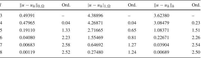
The results in Tables1,2,3and4match the theoretical results. In particular we
observe a first order convergence in the diffusion-dominated regime for the mesh (c),
as predicted by Theorem4, and a second order convergence in theL2norm of the error
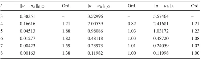
for both the convection and diffusion-dominated regimes. The latter is in accordance with the empirical observations that linearity preservation implies such a convergence. For mesh (d), which is non-symmetric, and hence the method is no longer linearity preserving, we can observe a first order convergence in both regimes. This convergence is not affected by the non-Delaunay character of the mesh.
We finish this example by a deeper study of the behavior of the nonlinear fixed-point
iteration with respect to the value of p. The results are reported in Table5. For these
results, we have used the three-directional mesh (c), withl=5. We can observe that,
for the values ofpranging from 1 to 10 the iterations needed to reach convergence are
essentially independent of the value ofp. This behavior is kept until a value around 20,
[image:20.439.51.389.503.601.2]and then some non-convergence is observed in the scheme. Here, by non-convergence we mean that the desired residual reduction has not been achieved after 5000 iterations. The same qualitative behavior has been observed for other meshes, and the two other settings presented later. In those cases, non-convergence has been observed starting at
Table 1 ε=10−6, numerical results for grid (c)
l u−uh0, Ord. |u−uh|1, Ord. u−uhh Ord.
3 0.49391 – 4.38896 – 3.62380 –
4 0.47965 0.04 4.26871 0.04 3.08479 0.23
5 0.19110 1.33 2.71665 0.65 1.08371 1.51
6 0.04080 2.23 1.55469 0.81 0.22671 2.26
7 0.00683 2.58 0.64692 1.27 0.03904 2.54
Table 2 ε=1, numerical results for grid (c)
l u−uh0, Ord. |u−uh|1, Ord. u−uhh Ord.
3 0.38594 – 3.48242 – 5.44504 –
4 0.16557 1.22 1.90920 0.87 2.26966 1.26
5 0.03268 2.34 0.89029 1.10 0.92785 1.29
6 0.00612 2.42 0.43637 1.03 0.43912 1.08
7 0.00141 2.12 0.21800 1.00 0.21818 1.01
[image:21.439.51.393.216.314.2]8 0.00035 2.02 0.10903 1.00 0.10904 1.00
Table 3 ε=10−6, numerical results for grid (d)
l u−uh0, Ord. |u−uh|1, Ord. u−uhh Ord.
3 0.48754 – 4.33607 – 5.06989 –
4 0.45680 0.09 4.11426 0.08 2.93242 0.79
5 0.17080 1.42 3.15455 0.38 1.05213 1.48
6 0.04330 1.98 2.23948 0.49 0.26065 2.01
7 0.01165 1.89 1.72410 0.38 0.05482 2.25
8 0.00474 1.30 1.63424 0.08 0.02087 1.39
Table 4 ε=1, numerical results for grid (d)
l u−uh0, Ord. |u−uh|1, Ord. u−uhh Ord.
3 0.38351 – 3.52996 – 5.57464 –
4 0.16616 1.21 2.00539 0.82 2.41681 1.21
5 0.04513 1.88 0.98086 1.03 1.03172 1.23
6 0.01277 1.82 0.48118 1.03 0.48720 1.08
7 0.00423 1.59 0.23973 1.01 0.24059 1.02
8 0.00163 1.38 0.11982 1.00 0.11998 1.00
Table 5 Iterations needed to reach convergence
p 1 2 3 4 5 6 7 8 9 10 15 20
Iter. 224 218 261 262 278 286 211 227 197 197 218 206
values of about 10 or 15, depending on the case. Then, we believe that it is safe to use
this scheme for values of p not much higher than 10. Of course, further work could
[image:21.439.50.392.350.450.2] [image:21.439.50.390.489.524.2]5.2 A problem with one inner layer, and a rotating convective field
We useε=10−5, f =0,σ =0, b=(−y,x), homogeneous Neumann boundary
conditions on exit, and
g(x,y)=
1 ifx≤0.5,
0 else,
as Dirichlet condition at entry. We have solved this problem on a uniform refinement
of the three-directional from mesh (c) in Fig.1. The parameterγ0has been set to 1,
and the results show no violation of the DMP. The results for this case are depicted in
Fig.2. We can observe that the increase in the value of pprovides a solution whose
inner layer is much sharper than the choice p =1. For both higher values for p, a
similar behaviour to the one in Table5was observed in terms of number of iterations
needed for convergence.
0 0.2 0.4 0.6 0.8
1 0.2 0
0.4 0.6 0.8 1 0 0.1 0.2 0.3 0.4 0.5 0.6 0.7 0.8 0.9 1 Approximate Solution (a) 0 0.2 0.4 0.6 0.8 1 0 0.2 0.4 0.6 0.8 1 0 0.1 0.2 0.3 0.4 0.5 0.6 0.7 0.8 0.9 1 Approximate Solution (b) 0 0.2 0.4 Approximate Solution 0 0.1 1 0.2 0.3 0.6 0.4 0.8 0.5 0.6 0.6 0.7 0.8 0.8 0.4 0.9 1
0.2 0 1
(c)
[image:22.439.54.381.276.582.2]0 0.1 0.2 0.3 0.4 0.5 0.6 0.7 0.8 0.9 1 0 0.51 0
0.1 0.2 0.3 0.4 0.5 0.6 0.7 0.8 0.9 1
Approximate Solution
(a)
0 0.1 0.2 0.3 0.4 0.5 0.6 0.7 0.8 0.9 1 0 0.5
1
0 0.1 0.2 0.3 0.4 0.5 0.6 0.7 0.8 0.9 1
Approximate Solution
(b)
1
Approximate Solution
0.5 0
0.1 0.2 0.3 0.4 0.5
0 0.6 0.7
0.2 0.8 0.9
0.4 1
0.6 0.8 1 0 (c)
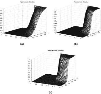
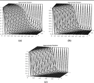
Fig. 3 Discrete solution forp=1 (top left) andp=4 (top right), andp=10 (bottom) 5.3 Advection skew to the mesh
We useε=10−5, f =0,σ =0b=cosπ3,sinπ3, and
g(x,y)=
1 ifx=0 or y=1,
0 else,
as Dirichlet condition. We have solved this problem on a criss-cross mesh as shown in
mesh (a) in Fig.1. We have used the parameterγ0=0.75, and, again, no violations of
the DMP have been observed. The results are depicted in Fig.3, where we can observe
much sharper layers (especially the internal one) when higher values forphave been
used. Again, for both higher values for p, a similar behaviour to the one in Table5
was observed in terms of number of iterations needed for convergence.
Acknowledgments The work of GRB and FK has been partially funded by the Leverhulme Trust via the Research Project Grant No. RPG-2012-483. The authors would like to thank Volker John and Petr Knobloch for very helpful discussions.
[image:23.439.56.386.45.336.2]and reproduction in any medium, provided you give appropriate credit to the original author(s) and the source, provide a link to the Creative Commons license, and indicate if changes were made.
References
1. Badia, S., Hierro, A.: On monotonicity-preserving stabilized finite element approximations of transport problems. SIAM J. Sci. Comput.36(6), A2673–A2697 (2014). doi:10.1137/130927206
2. Barrenechea, G.R., John, V., Knobloch, P.: Analysis of algebraic flux correction schemes. SIAM J. Numer. Anal. (2015, in press)
3. Barrenechea, G.R., John, V., Knobloch, P.: Some analytical results for an algebraic flux correction scheme for a steady convection–diffusion equation in one dimension. IMA J. Numer. Anal.35(4), 1729–1756 (2015). doi:10.1093/imanum/dru041
4. Burman, E.: On nonlinear artificial viscosity, discrete maximum principle and hyperbolic conservation laws. BIT47(4), 715–733 (2007). doi:10.1007/s10543-007-0147-7
5. Burman, E., Ern, A.: Nonlinear diffusion and discrete maximum principle for stabilized Galerkin approximations of the convection–diffusion–reaction equation. Comput. Methods Appl. Mech. Eng.
191(35), 3833–3855 (2002). doi:10.1016/S0045-7825(02)00318-3
6. Burman, E., Ern, A.: Discrete maximum principle for Galerkin approximations of the Laplace operator on arbitrary meshes. C. R. Math. Acad. Sci. Paris338(8), 641–646 (2004). doi:10.1016/j.crma.2004. 02.010
7. Burman, E., Ern, A.: Stabilized Galerkin approximation of convection–diffusion–reaction equations: discrete maximum principle and convergence. Math. Comput.74, 1637–1652 (2005)
8. Ern, A., Guermond, J.L.: Theory and Practice of Finite Elements. Springer, New York (2004) 9. Ern, A., Guermond, J.L.: Weighting the edge stabilization. SIAM J. Numer. Anal.51(3), 1655–1677
(2013). doi:10.1137/120867482
10. Gilbarg, D., Trudinger, N.S.: Elliptic partial differential equations of second order. In: Grundlehren der Mathematischen Wissenschaften [Fundamental Principles of Mathematical Sciences], vol. 224, 2nd edn. Springer, Berlin (1983). doi:10.1007/978-3-642-61798-0
11. Girault, V., Raviart, P.A.: Finite element methods for Navier–Stokes equations. In: Springer Series in Computational Mathematics, vol. 5. Springer, Berlin (1986). doi:10.1007/978-3-642-61623-5
12. Guermond, J.L., Nazarov, M.: A maximum-principle preservingC0finite element method for scalar conservation equations. Comput. Methods Appl. Mech. Eng.272, 198–213 (2014). doi:10.1016/j.cma. 2013.12.015
13. Guermond, J.L., Nazarov, M., Popov, B., Yang, Y.: A second-order maximum principle preserving Lagrange finite element technique for nonlinear scalar conservation equations. SIAM J. Numer. Anal.
52(4), 2163–2182 (2014). doi:10.1137/130950240
14. John, V., Knobloch, P.: On spurious oscillations at layers diminishing (SOLD) methods for convection– diffusion equations: part I—a review. Comput. Methods Appl. Mech. Eng.196, 2197–2215 (2007) 15. Kuzmin, D.: On the design of general-purpose flux limiters for finite element schemes. I. Scalar
convection. J. Comput. Phys.219, 513–531 (2006)
16. Kuzmin, D.: Algebraic flux correction for finite element discretizations of coupled systems. In: Papadrakakis, M., Oñate, E., Schrefler, B. (eds.) Proceedings of the Int. Conf. on Computational Methods for Coupled Problems in Science and Engineering, pp. 1–5. CIMNE, Barcelona (2007) 17. Kuzmin, D.: Linearity-preserving flux correction and convergence acceleration for constrained
Galerkin schemes. J. Comput. Appl. Math.236, 2317–2337 (2012)
18. Kuzmin, D., Hämäläinen, J.: Finite element methods for computational fluid dynamics. In: Compu-tational Science and Engineering, vol. 14. Society for Industrial and Applied Mathematics (SIAM), Philadelphia (2015). (A practical guide)
19. Kuzmin, D., Turek, S.: Flux correction tools for finite elements. J. Comput. Phys.175(2), 525–558 (2002). doi:10.1006/jcph.2001.6955
20. Löhner, R., Morgan, K., Vahdati, M., Boris, J.P., Book, D.L.: FEM-FCT: combining unstructured grids with high resolution. Commun. Appl. Numer. Methods4(6), 717–729 (1988). doi:10.1002/cnm. 1630040605
22. Xu, J., Zikatanov, L.: A monotone finite element scheme for convection–diffusion equations. Math. Comput.68(228), 1429–1446 (1999). doi:10.1090/S0025-5718-99-01148-5
23. Zalesak, S.T.: Fully multidimensional flux-corrected transport algorithms for fluids. J. Comput. Phys.