A cost-benefit approach for the evaluation of prognostics-updated maintenance strategies in complex dynamic systems

A cost-benefit approach for the evaluation of prognostics-updated

maintenance strategies in complex dynamic systems

Jose Ignacio Aizpurua & Victoria M. Catterson

Department of Electronic & Electrical Engineering - Institute for Energy & Environment University of Strathclyde, Glasgow, UK

Ferdinando Chiacchio & Diego D’Urso

Universit´a di Catania, Catania, Italy

ABSTRACT: The implementation of maintenance strategies which integrate online condition data has the po-tential to increase availability and reduce maintenance costs. Prognostics techniques enable the implementation of these strategies through up-to-date remaining useful life estimations. However, a cost-benefit assessment is necessary to verify the scale of potential benefits of condition-based maintenance strategies and prognostics for a given application. The majority of prognostics applications focus on the evaluation of a specific failure mode of an asset. However, industrial systems are comprised of different assets with multiple failure modes, which in turn, work in cooperation to perform a system level function. Besides, these systems include time-dependent events and conditional triggering events which cause further effects on the system. In this context not only are the system-level prognostics predictions challenging, but also the cost-benefit analysis of condition-based maintenance policies. In this work we combine asset prognostics predictions with temporal logic so as to obtain an up-to-date system level health estimation. We use asset level and system level prognostics estimations to evaluate the cost-effectiveness of alternative maintenance policies. The application of the proposed approach enables the adoption of conscious trade-off decisions between alternative maintenance strategies for complex systems. The benefits of the proposed approach are discussed with a case study from the power industry.

1 INTRODUCTION

Prognostics is an emerging field with potential economic benefits for maintenance (Vachtsevanos, Lewis, Roemer, Hess, & Wu 2007). Prognostics ap-proaches predict the Remaining Useful Life (RUL) of the asset under study, which can help to extend the useful life of assets improving availability and reduc-ing maintenance costs (Aizpurua & Catterson 2015b). Cost-effective maintenance strategies minimize RUL waste without hazardous consequences (Had-dad, Sandborn, & Pecht 2012). In order to justify the implementation of a maintenance strategy, cost-benefit assessments are needed to compare their per-formance and select the most effective strategy.

In this paper we analyse the cost-effectiveness of different maintenance strategies including reac-tive, reliability-centred and condition-based mainte-nance (Kobbacy & Murthy 2008). In reactive main-tenance the asset is repaired after its failure oc-currence. Reliability-centred maintenance strategies monitor the failure probability of the asset to

de-fine preventive replacement policies based on failure probability thresholds. Condition-based maintenance strategies make use of prognostics predictions to de-fine preventive maintenance actions.

Maintenance strategies can be implemented at dif-ferent hierarchical levels. While system-level mainte-nance includes system health information, asset-level strategies concentrate on asset health estimation. In this paper we will focus on asset-level maintenance.

Industrial systems are no longer characterized with static operation logic. Instead, they involve complex interactions that affect the system dependability and include repair/maintenance events for different assets. In this paper we will focus on Dynamic Fault Tree logic to analyse the system failure probability caused by the failure of assets (Manno, Chiacchio, Com-pagno, D’Urso, & Trapani 2014).

The remainder of this paper is organised as fol-lows. Section 2 presents related work. Section 3 presents the cost-benefit approach for maintenance of dynamic systems. Section 4 applies the proposed ap-proach to a transmission substation case study. Sec-tion 5 discusses challenges for system-level mainte-nance strategies with dynamic scenarios and finally, Section 6 presents conclusions and future prospects.

2 RELATED WORK

Different dependencies arise when implementing maintenance strategies for multi-component systems (Thomas 1986). Stochastic dependency implies that the deterioration of an asset impacts the performance of other assets; structural dependency means that maintaining a component implies the maintenance (or unavailability) of other components; and economic dependency addresses the difference between group and independent maintenance actions.

The main goal of maintenance strategies is to max-imize availability and minmax-imize risk and cost. To this end, alternative approaches have been presented fo-cused on the optimization of maintenance parameters. Many of the condition-based maintenance approaches propose analytical formulations that integrate degra-dation models within the maintenance modelling ap-proach and monitor the failure threshold to establish preventive maintenance actions (Grall, B´erenguer, & Dieulle 2002). Other approaches make use of meta-heuristics for the optimization process with additional constraints such as available resources (Camci 2009). With the advance of prognostics approaches, the in-terest in condition-based maintenance approaches has increased. (Haddad, Sandborn, & Pecht 2012) imple-mented Monte Carlo simulations for the cost-benefit analysis of condition-based maintenance strategies. Options theory is used to evaluate maintenance de-cisions after RUL prediction, which enable the quan-tification of the value of waiting to maintain.

Multi-level maintenance strategies have recently gained the interest of researchers as a possibility to re-duce maintenance costs by grouping assets. (Nguyen, Do, & Grall 2015) presents a multi-level preven-tive maintenance decision making algorithm. At each inspection time, conditional probabilities are calcu-lated to update the system-level reliability modelled with Reliability Block Diagrams (RBD). At compo-nent level, a cost-based group improvement factor is used to define preventive maintenance actions. (Do, Vu, Barros, & B´erenguer 2015) combines corrective and preventive maintenance actions for the optimal scheduling of personnel and optimal grouping of as-sets. A genetic algorithm is used to integrate limited personnel and downtime durations which can change over time. The system is assumed to be a series model and the failure behaviour of system components is defined by Weibull distributions. (Vu, Do, & Barros 2016) make use of Birnbaum importance measures

and mean residual life for system-level maintenance strategies. Assets are grouped for maintenance de-pending on if the failure of a component can cause the system failure. RBD logic is used to express the functional/failure operation of the system.

(Do, Voisin, Levrat, & Iung 2015) evaluates the effect of perfect and imperfect maintenance for condition-based maintenance. An adaptive mainte-nance policy is proposed to select optimal main-tenance actions at each inspection time. Inspection times are based on RUL estimations, so that sys-tem failure probability before next inspection remains lower than a threshold. Failure probability between inspection times, imperfect and preventive mainte-nance thresholds are the optimization variables. Un-limited resources, negligible maintenance durations, and a Gamma degradation process are assumed.

Petri nets have also been used to evaluate the effect of different maintenance parameters on system per-formance for different maintenance strategies. (Zille, B´erenguer, Grall, & Despujols 2011) evaluated relia-bility centred maintenance strategies using Petri nets. Similarly, (Andrews, Prescott, & Rozires 2014) pre-sented a Petri net model extended with three addi-tional transition types for railway track asset man-agement. Analysed parameters include inspection, re-newal, and repair times and maintenance threshold.

All the analysed system-level models take into account the combinatorial failure logic of the sys-tem (Nguyen, Do, & Grall 2015, Do, Vu, Barros, & B´erenguer 2015, Vu, Do, & Barros 2016). Besides, most of the reviewed approaches integrate a degra-dation process to model the degradegra-dation of the asset and facilitate the posterior analytical treatment (Grall, B´erenguer, & Dieulle 2002, Haddad, Sandborn, & Pecht 2012, Do, Vu, Barros, & B´erenguer 2015, Do, Voisin, Levrat, & Iung 2015). This may limit their practicality for different degradation processes.

The main contribution of this paper is the evalu-ation of prognostics-updated maintenance strategies in complex dynamic systems. These systems are more complex than systems with combinatorial fail-ure logic, because they involve stochastic and tem-poral dependencies between events. The evaluation of these systems is achieved through the integration of degradation-independent prognostics models with maintenance models. This provides benefits for main-tenance modelling enabling the use of different types of degradation processes and prognostics models.

In this paper we will not focus on optimization al-gorithms because this requires the conception of an analytic formulation for dynamic and repairable sys-tems (see Section 5).

3 MAINTENANCE MODELS FOR DYNAMIC RELIABILITY SCENARIOS

fail-ure logic, prognostics prediction results, and metrics extracted at asset and system level.

W

M F

1(t)

1(t)

1(t)

1(t)

Asset1

W

M F

2(t)

2(t)

2(t)

2(t)

Asset2

W

M F

i(t)

i(t)

i

(t)

i

(t)

Asseti

Dynamic Failure Logic System Failure

Component-level Metrics System-level Metrics

Figure 1: Proposed maintenance approach.

Each asset is modelled with three states. The transi-tion from working (W) to failed (F) state is governed by the failure rate λ(t). This failure rate can be up-dated with up-to-date degradation prediction informa-tion. Once the asset fails, it is repaired with a repair rateµ(t), which models the mean time to repair from failed to working state.

It is possible to avoid the transition to the failed state by performing maintenance prior to the asset failure occurrence. The transition to the maintenance state (M) depends on the maintenance strategy and it is determined by the transition rateω(t). Once in the maintenance state, the asset needs a time interval de-fined byθ(t)to return back to the working state.

For asset-level reliability centred maintenance strategiesω(t)is dependent on the asset failure prob-ability. Namely, the asset maintenance is triggered when the failure probability of the asset is above a predefined failure threshold.

As for asset-level condition-based maintenance strategies, ω(t) is defined as (Aizpurua & Catterson 2015a):

ω(t) =RU L(Tp)−SF (1)

whereRU Lis remaining useful life at prediction time

Tp andSF is a safety factor which integrates

uncer-tainties associated with the RUL prediction.

We calculate the failure probability and cost for each asset as cost-benefit indicators. The failure prob-ability is computed at runtime through the Cumulative Distribution Function (CDF). From basic reliability theory the CDF is defined as:

FX(x) =P(X≤x) =

Z x

0

fx(t)dt (2)

where X is a random variable of the time to failure andxis the current time instant.

The cost function for each assetiis defined as:

Ci(t)=ci+cpsd+cd×d+cusd+mi(t)+sm+uCBM (3)

where,

• ci: cost of the asseti.

• cpsd: planned shutdown cost due to maintenance.

• cd: downtime cost rate,d: downtime.

• cusd: unplanned shutdown cost due to failure.

• mi(t): deterioration cost,mi(t) =cdet×P r(f ail)

andcdetis the deterioration cost rate.

• sm: initial maintenance setup cost.

• uCBM: cost for updating maintenance plans at

runtime (e.g. with prognostics predictions).

Finally, the system-level cost is calculated as the sum of the cost of each asset:

Costsystem(t) = N

X

i=1

Ci(t) (4)

whereN is the total number of assets in the system. The main assumptions adopted in this paper are: assets are in as bad as old state after repair and avail-ability of unlimited maintenance resources.

We use Stochastic Activity Networks (SAN) (Sanders & Meyer 2001) to integrate prognostics re-sults, maintenance strategies, dynamic reliability and reconfiguration logic in a single model. SAN is a very flexible formalism which can model complex mainte-nance strategies. Due to space limitations, in this pa-per we will emphasize maintenance modelling con-cepts.

3.1 Preliminaries on Stochastic Activity Networks

Stochastic Activity Networks (SAN) extends stochas-tic Petri Nets generalizing stochasstochas-tic relationships and adding mechanisms for hierarchical modelling. Fig-ure 2 shows SAN elements (Sanders & Meyer 2001).

Standard Place Extended Place Input Gate Output Gate

Join

Join

Instantaneous

Activity ActivityTimed

Submodel

model Atomic/ Composed

Figure 2: Notation of SAN modelling elements.

Placesrepresent the state of the modelled system. Each place contains a certain number of tokens defin-ing the markdefin-ing of the place. A standard place con-tains an integer number of tokens, whereasextended

There are two types of activities: instantaneous

which complete in negligible amount of time and

timedwhose duration has an effect on the system per-formance and their completion time can be a constant or a random value. When it is a random value, it is ruled by a probability distribution function defining the time to fire the activity.

Activitiesfire based on the conditions defined over the marking of the net and their effect is to modify the marking of the places. The completion of an activity of any kind is enabled by a particular marking of a set of places. The presence of at least one token in each input place enables the firing of the activity remov-ing the token from its input place(s) and placremov-ing them in the output place(s). Each activity has a reactiva-tion funcreactiva-tionthat defines when the activity is aborted and a new activity time is immediately obtained from the activity time distribution. The reactivation func-tion provides a mechanism for restarting activities if the reactivation predicate holds for the new marking and for the marking in which the activity was origi-nally activated; and the activity remains enabled.

Another way to enable a certain activity consists ofInput Gates (IGs)andOutput Gates (OGs). These gates make the SAN formalism general and powerful enough to model complex real situations. They de-termine the marking of the net based on user-defined C++ rules. IGscontrol the enabling of activities and define the marking changes that will occur when an activity completes. A set of places is connected to the

IGand theIGis connected to an activity. A Boolean condition enables the activity connected to the gate and a function determines the effect of the activity completion on the marking of the places connected to the gate. OGs specify the effect of activity com-pletion on the marking of the places connected to the OG. An output function defines the marking changes that occur when the activity completes.

The SAN models which include the specified SAN elements are modelled in a SANatomic model. The

join operatorlinks through a compositional tree struc-ture different SAN models in a unique composed model. It is possible to link atomic models, composed models, or combinations thereof. In the tree structure, the composed and atomic SAN models are linked through join operators using shared places between the composed and atomic SAN models.

The performance measurements are carried out through reward functions defined over the designed model. Reward functions are defined based on the marking of the net or completion of activities and they are evaluated as the expected value of the re-ward function. For a complete and formal definition of SAN please refer to (Sanders & Meyer 2001).

For the sake of clarity, in subsequent figures, we will designate timed activities and we will hide the label of instantaneous activities (cf. Figs. 3-5).

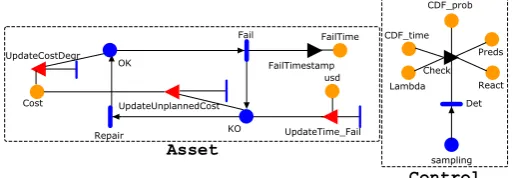
3.2 Reactive maintenance model

Reactive maintenance repairs the asset as soon as it fails without preventive maintenance actions. Figure 3 shows the reactive maintenance model comprised ofAssetandControlblocks.

KO OK

UpdateTime_Fail UpdateCostDegr

FailTimestamp

Repair

Fail

usd FailTime

Cost UpdateUnplannedCost

Asset

sampling React Lambda

Preds CDF_prob

CDF_time

Check

Det

Control

Figure 3: Reactive maintenance model.

The Asset model transits between OK and KO places according toFailandRepairtimed activities. TheFailactivity is updated (reactivated in SAN ter-minology) according to prognostics prediction results (λ(t) in Fig 1). The FailTimestamp OG calculates the failure time instant andUpdateTime FailIG cal-culates downtime of the asset recorded respectively in the extended places named FailTime and usd. According to Eq. (3), UpdateUnplannedCost and UpdateCostDegr IGs calculate cusd and mi(t)

re-spectively, both recorded in theCostextended place. The core of the Controlblock is the Check OG. It implements the online CDF calculation and it up-dates the failure degradation trend with prognostics prediction results. The timed activityDetexecutes the CheckOG at∆t timesteps during the mission time.

On the one hand, for the online CDF calculation, if we assume that the asset under study degrades ac-cording to the exponential distribution, Eq. (5) shows the CDF of the exponential distribution:

F(t) = 1−e(−λt) (5)

whereλis the failure rate parameter.

Accordingly,CDF timeandCDF probplaces store the time to failure of the asset and the online failure probability respectively. Note that the constant failure rate can be approximated as the inverse of the RUL (λ≈1/RU L) (Banjevic & Jardine 2006).

On the other hand, theCheckOG evaluates if there is any prognostics prediction that needs to be updated according to prognostics prediction results. Prognos-tics prediction values and prediction time instants are stored in the extended place Preds (cf. Table 1). If the simulation time instant coincides with the predic-tion time instant Tp, then the marking of theLambda

extended place is updated with prognostics prediction values and the Fail activity is reactivated with the updated marking of theLambdaextended place.

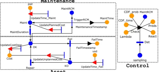
3.3 Reliability-centred maintenance model

the PDF integration algorithm (Chiacchio, D’Urso, Manno, & Compagno 2016), and when it passes a threshold, maintenance is triggered. Figure 4 shows the RCM maintenance model divided into Asset, ControlandMaintenanceblocks.

Maint

UpdatePlannedCost UpdateTime_Maint

MaintenanceTimestamp

MaintDuration psd

MaintTime TriggerRCM

MaintRCM

KO OK

UpdateTime_Fail UpdateCostDegr

FailTimestamp

Repair

Fail

usd FailTime

Cost UpdateUnplannedCost

Asset Maintenance

MaintRCM

sampling React Lambda

Preds CDF_prob

CDF_time

Check

Det

Control

Figure 4: Reliability centred maintenance model.

The Asset block is the same as in the reactive maintenance model. The Control block integrates theMaintRCMplace, which is activated when the fail-ure probability modelled by the CDF prob extended place is above a predefined maintenance threshold.

The Maintenance block performs preventive maintenance according to the MaintRCM place. That is, if the asset is in the OK place and MaintRCM is activated, the asset goes through planned main-tenance (ω(t) in Fig. 1) passing through the Maint place and MaintDuration activity (θ(t) in Fig. 1). After performing maintenance, the asset returns back to the OK place. The MaintenanceTimestamp OG registers the maintenance time instant and the UpdateTime MaintIG calculates the planned down-time stored in MaintTime and psdextended places, respectively. Accordingly, the UpdatePlannedCost IG calculates the planned cost due to maintenance.

3.4 Condition-based maintenance model

Figure 5 shows the Condition-Based Maintenance (CBM) model divided into Asset, Control, and Maintenanceblocks.

The Asset block integrates OK, KO, StandBy and Activate places with Fail and Repair timed activities and an instantaneous activity link-ing StandBy and Activate places. It updates the system cost via UpdateUnplannedCost and UpdateCostsDegr IGs. Failure instants are calcu-lated with the FailTimestamp OG and unplanned downtimes are calculated with theUpdateTime Fail IG. TheFailactivity is updated with prognostics pre-diction results with degradation prepre-dictions stored in thePredsplace. When the asset is repaired, it remains in theStandBystate until it receives anActivate sig-nal from the reconfiguration mechanism.

TheControlblock models the system update and online CDF calculation through the Check OG. The Failand MaintCBMactivities (λ(t)and ω(t)in Fig. 1, respectively) are reactivated and updated with new

transition rates via theLambdaandLambda Mplaces, respectively. The SF place stores the safety factor to update the maintenance places (cf. Eq. (1)). The CDF timeandCDF probplaces model the online cal-culation of the CDF according to Eq. (2).

TheMaintenanceblock implements planned shut-down events. TheMaintCBMtimed activity models the

ω(t) event in Figure 1. MaintCBM has a reactivation logic to update the transition rate to theMaint place according to prognostics prediction results and pre-diction instants stored in the Preds place (Control block). MaintDuration activity models the θ(t)

event in Figure 1. The UpdateTime Maint and UpdatePlannedCost IGs calculate planned down-time and cost, respectively.

4 CASE STUDY

The correct operation of a transmission substation is critical for power grid performance. Figure 6 shows a configuration example of a transmission substation.

The repair of the transformer is a very expensive and time consuming process (CIGR ´E 2015). Accord-ingly, the transmission substation is designed to be a fault tolerant system. In the configuration shown in Figure 6, there are always two active transformers and other two are in standby mode. Anytime an active transformer fails, a standby transformer is activated.

Prognostics indicators for transformers and circuit breakers can be extracted from different degradation indicators (e.g. (Catterson, Melone, & Garcia 2016)) and a suitable prognostics prediction model can be chosen according to a prognostics model selection process (Aizpurua & Catterson 2015b). However, for simplicity, hypothetical prognostics prediction values displayed in Table 1 are adopted at these prediction instants (Tp); Tp1: 6 years for the circuit breaker; 8

years for the transformer; and Tp2: 12 years for the

circuit breaker; 16 years for the transformer.

Table 1: RUL values (in years) at prediction timesTp.

Assets Tr1 Tr2 Tr3 Tr4 CB1 CB2 CB3 CB4

Tp0 15 15 15 15 1 1 1 1

Tp1 12 13 18 20 0.6 0.5 0.9 0.9

Tp2 9 10 16 18 0.5 0.4 0.7 0.7

For circuit breakers theAssetmodel in Figures 3 and 4 is implemented and for transformers theAsset model in Figure 5 is implemented with standby states (i.e. as the Component-level Metrics of Fig. 1). The reconfiguration logic implements the priority of trans-formers. Anytime a transformer fails, the transformer with the highest priority is activated. If a transformer with a higher priority is repaired, it remains in the standby state until a lower priority transformer fails.

KO OK

StandBy Activate Maint

UpdatePlannedCost UpdateTime_Maint

UpdateTime_Fail UpdateCostDegr

FailTimestamp MaintenanceTimestamp

Repair

Fail MaintCBM

MaintDuration

usd FailTime

Cost psd

MaintTime

UpdateUnplannedCost

sampling React

Lambda_M Lambda

Preds SF CDF_prob CDF_time

Check

Det

Control

Asset Maintenance

Figure 5: Condition-based maintenance model.

Busbar

Transf.

Tr1 CB1

Transf.

Tr2 CB2

Transf.

Tr3 CB3

Transf.

Tr4 CB4

Figure 6: Transmission substation.

Muxika, Papadopoulos, Chiacchio, & Manno 2016). However, for repairable systems, the number of pos-sible reconfiguration strategies increases due to the stochastic nature of failure and repair events. The re-configuration logic has been implemented in SAN ac-cording to the priority of transformers and possible failure and repair events. Namely, when a standby transformer needs to be activated, the marking of the correspondingActivateplace is set (cf. Fig. 5).

TheControlandMaintenanceblocks depend on the specific maintenance strategy to be analysed.

The failure condition of the transmission substa-tion in Figure 6 can be expressed using Dynamic Fault Tree (DFT) gates (Manno, Chiacchio, Com-pagno, D’Urso, & Trapani 2014):

(a) PAND:Y =P AN D(E1,. . . ,EN); Y istrueiff all

events {E1, . . . , EN} are true and they occur in

order:E1/. . ./ EN; otherwise isfalse(cf. Fig. 7a).

(b) Spare: Y =SP(Eact1,. . .,EactM,Esp1, . . . , EspN);

Y is true iff all active events {Eact1,. . .,EactM}

and all spare events {Esp1,. . .,EspN} have failed,

otherwise is false. Its inputs can be in any of the following three states: standby, working or failed (cf. Fig. 7b).

(c) SEQ:SEQ(E1,. . .,EN); {E1,. . .,EN}are true iff

all events {E1,. . .,EN} are true and occur in the

following order:E1/. . ./EN (cf. Fig. 7c).

(d) FDEP:[E1,. . .,EN] =F DEP(T);{E1,. . .,EN}is

true if the trigger event T occurs or they fail by themselves; otherwise isfalse(cf. Fig. 7d).

Figure 8 defines the failure condition of the trans-mission substation shown in Figure 6 (i.e. Dynamic Failure Logic in Fig. 1), which can be interpreted as follows. The system failure will occur either because:

(a) PAND Gate

Figure 7: Dynamic Fault Tree gates.

(i) Two transformers fail and two complementary circuit breakers have already failed (IE1-IE6).

(ii) One transformer fails and three complementary circuit breakers have already failed (IE7-IE10).

(iii) All transformers fail (spare gate).

The spare gate determines the activation priority of the inputs from left to right order. That is, any time Tr1is available, its activation is preferred over the rest

of transformers which are in standby state.

We have used the DFT model in Figure 8 to eval-uate the system failure probability with prognostics predictions in Table 1 andω=0.8 yrs;θ=1 yrs (Fig. 1). Table 2 displays analysed maintenance scenarios (SC) with different maintenance strategies and dif-ferent safety factor (SF) and maintenance threshold values. So as to evaluate the effect of uncertainty on CBM strategies, we have used different SF values for transformers (SFTr) and circuit breakers (SFCB),

re-specting the proportionality in Table 1 (SFTr>SFCB).

For RCM scenarios we have used two different failure probability values to analyse the effect of replacing assets with different degradation levels.

Table 2: Analysed maintenance scenarios.

Scenario Strategy Parameters

SC1 Reactive N/A

SC2 CBM SFCB=0.3 year; SFTr=5 years

SC3 CBM SFCB=0.1 year; SFTr=1 year

SC4 RCM Maintenance Threshold=0.9 SC5 RCM Maintenance Threshold=0.95

Substation Failure

Tr4

CB2CB3 CB1 Tr3

CB2CB4 CB1 Tr2

CB3CB4 CB1 Tr1

CB3CB4 CB2 Tr1

CB4 CB2

Tr3

CB4 CB2

Tr1

CB3 CB2

Tr4

CB3 CB2

Tr2

CB4 CB1

Tr3

CB4 CB1

Tr2

CB3 CB1

Tr4

CB3 CB1

Tr3

CB2 CB1

Tr4

CB2 CB1 Tr1

CB4 CB3

Tr2

CB4 CB3

Tr1Tr2Tr3Tr4

IE1 IE2 IE3 IE4 IE5 IE6 IE7 IE8 IE9 IE10

Figure 8: Dynamic Fault Tree model of the transmission substation in Figure 6.

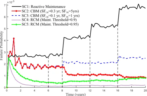
Time (years)

0 2 4 6 8 10 12 14 16 18 20

Failure Probability

×10-3

0 1 2 3 4 5 6 7

SC3: CBM (SFCB=0.1 yr, SFTR=1 yrs)

SC2: CBM (SFCB=0.3 yr; SFTR=5yrs)

SC1: Reactive Maintenance

SC4: RCM (Maint. Threshold=0.9) SC5: RCM (Maint. Threshold=0.95)

Figure 9: Failure probabilities of maintenance strategies.

With CBM the failure probability of the system is reduced with respect to reactive maintenance because the maintenance is adapted according to new prognos-tics predictions (cf. Eq. (1)). The effect of the safety factor on the failure probability shows that the bigger the safety margin, the lower the failure probability of the system, i.e. maintenance is done more frequently. With RCM the system failure probability is even lower than CBM because the maintenance of the as-set is performed more frequently. Accordingly, the greater the maintenance threshold, the greater the fail-ure probability because the asset is left to run longer.

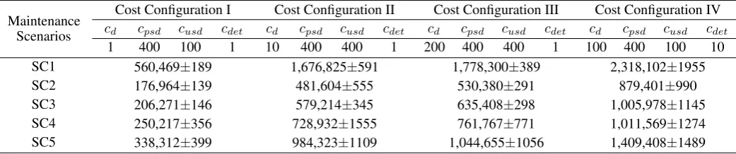
For each scenario in Table 2, we have analysed the total cost of the system displayed in Table 3. For each asset we have evaluated its cost according to Eq. (3) and then we have computed the total system cost ac-cording to Eq. (4). We have analysed different cost values for cost variables in Eq. (3) and we have as-sumed as constant the remainder of cost variables not shown in Table 3 (i.e.ci,sm, anduCBM).

As Table 3 displays, the most expensive strategy is the reactive maintenance strategy. On the other hand, the most economic configuration is the CBM strat-egy. CBM is cheaper than RCM because the main-tenance activity is triggered less frequently and the failure probability difference with respect to the RCM strategy is not relevant (cf. Figure 9).

The effect of the deterioration cost rate (cdet) is also

worth mentioning. If we compare cost I and cost IV configurations, variations in cdet and downtime cost

rates (cd) have a representative impact on the final

cost. In contrast, if we compare configurations II and

III, we can see that decreasing the downtime cost rate (cd) impacts slightly on the final cost.

If we compare the cost configurations III and IV, we notice that, if we increase the deterioration cost rate (cdet), even decreasing the downtime cost rate (cd) and

unplanned shutdown cost value (cusd), the cost of the

system increases. The contribution of the deteriora-tion cost rate is more relevant than the downtime cost rate (cd) and unplanned shutdown cost value (cusd).

5 DISCUSSION

In this paper, the difference between RCM and CBM strategies resides in the maintenance triggering con-dition. Both strategies require monitoring the degra-dation trend of the asset under study. Traditionally, this degradation trend has been considered as a prede-fined degradation process (see Section 2). However, as shown in this paper, with the recent advance of prognostics approaches, there is room to tailor these maintenance strategies with up to date prognostics prediction results including results coming from dif-ferent prognostics approaches (see Figure 9).

Transition from asset-level to system-level mainte-nance strategies is a challenging task with dynamic failure scenarios. An important indicator for decision making of system-level maintenance strategies is to analyse if the failure of an asset can cause the system failure. With static systems this can be evaluated using minimal cut-set concepts (Vu, Do, & Barros 2016). However, in the context of dynamic repairable scenar-ios, it is necessary to analyse Minimal Cut Sequence Sets (MCSSs) (Walker & Papadopoulos 2009).

MCSSs have been analysed for non-repairable DFT gates (Merle, Roussel, & Lesage 2011). However, the analytic solution for repairable systems is complex and remains unsolved. In this context, the capability to check if the failure of an asset causes the system failure would enable the classification of assets ac-cording to their criticality and it would facilitate the conception of maintenance grouping strategies (i.e. economic and structural dependencies, see Section 2).

6 CONCLUSIONS

Table 3: Cost sensitivity analysis at T=20 years.

Maintenance Scenarios

Cost Configuration I Cost Configuration II Cost Configuration III Cost Configuration IV

cd cpsd cusd cdet cd cpsd cusd cdet cd cpsd cusd cdet cd cpsd cusd cdet

1 400 100 1 10 400 400 1 200 400 400 1 100 400 100 10 SC1 560,469±189 1,676,825±591 1,778,300±389 2,318,102±1955 SC2 176,964±139 481,604±555 530,380±291 879,401±990 SC3 206,271±146 579,214±345 635,408±298 1,005,978±1145 SC4 250,217±356 728,932±1555 761,767±771 1,011,569±1274 SC5 338,312±399 984,323±1109 1,044,655±1056 1,409,408±1489

Current systems integrate not only time-dependent operations, but also inter-dependent mechanisms, where the failure of one asset activates another mech-anism. With the recent advance of prognostics ap-proaches, it is possible to implement condition-based maintenance strategies tailored to specific operation conditions. Integrating all these elements, the com-bination of dynamic failure scenarios and condition-based maintenance strategies poses new challenges.

In this paper we have integrated prognostics pre-diction results with Dynamic Fault Tree models and we have analysed different maintenance strate-gies implemented at the asset level. Stochastic Ac-tivity Networks have been used for the evalua-tion of the cost-effectiveness of different mainte-nance strategies. Analysed maintemainte-nance strategies include reactive, reliability-centred and condition-based maintenance strategies. In the realized ex-periments, reliability-centred maintenance strategies show a lower failure probability, but a higher cost compared with condition-based maintenance strate-gies. Reactive maintenance is the most expensive strategy with the highest failure probability.

In future work we will move from component-level to system-level maintenance strategies, so as to eval-uate cost-benefit indicators in complex dynamic sys-tems at different hierarchical levels.

REFERENCES

Aizpurua, J. I. & V. M. Catterson (2015a, Dec). On the use of probabilistic model-checking for the verification of prognos-tics applications. InIEEE International Conference on Intel-ligent Computing and Information Systems, pp. 7–13. Aizpurua, J. I. & V. M. Catterson (2015b, Oct). Towards a

methodology for design of prognostics systems. InAnnual Conf. of the Prognostics and Health Management Society. Aizpurua, J. I., E. Muxika, Y. Papadopoulos, F. Chiacchio,

& G. Manno (2016). Application of the D3H2 Methodol-ogy for the Cost-Effective Design of Dependable Systems.

Safety 2(2), 9.

Andrews, J., D. Prescott, & F. D. Rozires (2014). A stochastic model for railway track asset management.Reliability Engi-neering & System Safety 130, 76 – 84.

Banjevic, D. & A. K. S. Jardine (2006). Calculation of reliability function and remaining useful life for a markov failure time process. IMA Journal of Management Mathematics 17(2), 115–130.

Camci, F. (2009). System maintenance scheduling with prognos-tics information using genetic algorithm.IEEE Transactions on Reliability 58(3), 539–552.

Catterson, V. M., J. Melone, & M. S. Garcia (2016, January). Prognostics of transformer paper insulation using statistical particle filtering of on-line data.IEEE Electrical Insulation Magazine 32(1), 28–33.

Chiacchio, F., D. D’Urso, G. Manno, & L. Compagno (2016). Stochastic hybrid automaton model of a multi-state system with aging: Reliability assessment and design consequences.

Reliability Engineering & System Safety 149, 1–13. CIGR ´E (2015).Transformer Reliability Survey. Number 642. Do, P., A. Voisin, E. Levrat, & B. Iung (2015). A proactive

condition-based maintenance strategy with both perfect and imperfect maintenance actions. Reliability Engineering & System Safety 133, 22 – 32.

Do, P., H. C. Vu, A. Barros, & C. B´erenguer (2015). Main-tenance grouping for multi-component systems with avail-ability constraints and limited maintenance teams.Reliability Engineering & System Safety 142, 56 – 67.

Grall, A., C. B´erenguer, & L. Dieulle (2002). A condition-based maintenance policy for stochastically deteriorating systems.

Reliability Engineering & System Safety 76(2), 167 – 180. Haddad, G., P. A. Sandborn, & M. G. Pecht (2012). An options

approach for decision support of systems with prognostic ca-pabilities.IEEE Transactions on Reliability 61(4), 872–883. Kobbacy, K. & D. Murthy (2008).Complex System Maintenance

Handbook. Springer Series in Reliability Eng. Springer. Manno, G., F. Chiacchio, L. Compagno, D. D’Urso, & N.

Tra-pani (2014). Conception of Repairable Dynamic Fault Trees and resolution by the use of RAATSS, a MatlabR _toolbox

based on the ATS formalism.Reliability Engineering & Sys-tem Safety 121, 250 – 262.

Merle, G., J.-M. Roussel, & J.-J. Lesage (2011). Algebraic de-termination of the structure function of dynamic fault trees.

Reliability Engineering & System Safety 96(2), 267 – 277. Nguyen, K.-A., P. Do, & A. Grall (2015). Multi-level predictive

maintenance for multi-component systems.Reliability Engi-neering & System Safety 144, 83 – 94.

Sanders, W. H. & J. F. Meyer (2001). Stochastic activity net-works: Formal definitions and concepts. InLectures on For-mal Methods and Performance Analysis, Volume 2090 of

LNCS, pp. 315–343. Springer Berlin Heidelberg.

Thomas, L. (1986). A survey of maintenance and replacement models for maintainability and reliability of multi-item sys-tems.Reliability Engineering 16(4), 297 – 309.

Vachtsevanos, G., F. Lewis, M. Roemer, A. Hess, & B. Wu (2007).Intelligent Fault Diagnosis and Prognosis for Engi-neering Systems. John Wiley & Sons, Inc.

Vu, H. C., P. Do, & A. Barros (2016). A stationary group-ing maintenance strategy usgroup-ing mean residual life and the birnbaum importance measure for complex structures.IEEE Transactions on Reliability 65(1), 217–234.

Walker, M. & Y. Papadopoulos (2009). Qualitative temporal analysis: Towards a full implementation of the fault tree handbook.Control Eng. Practice 17(10), 1115–1125. Zille, V., C. B´erenguer, A. Grall, & A. Despujols (2011).