Creep rupture assessment by a robust creep data interpolation using the linear matching method

Creep rupture assessment by a robust creep data interpolation using the

Linear Matching Method

Daniele Barbera, Haofeng Chen*

Department of Mechanical & Aerospace Engineering, University of Strathclyde, Glasgow G1 1XJ, UK

Abstract

The accurate assessment of creep rupture limit is an important issue for industrial components under combined action of cyclic thermal and mechanical loading. This paper proposes a new creep rupture assessment method under the Linear Matching Method framework, where the creep rupture limit is evaluated through an extended shakedown analysis using the revised yield stress, which is determined by the minimum of the yield stress of the material and the individual creep rupture stress at each integration point. Various numerical strategies have been investigated to calculate these creep rupture stresses associated with given temperatures and allowable creep rupture time. Three distinct methods: a) linear interpolation method, b) logarithm based polynomial relationship and c) the Larson Miller parameter, are introduced to interpolate and extrapolate an accurate creep rupture stress, on the basis of discrete experimental creep rupture data. Comparisons between these methods are carried out to determine the most appropriate approach leading to the accurate solution to the creep rupture stresses for the creep rupture analysis. Two numerical examples including a classical holed plate problem and a two-pipe structure are provided to verify the applicability and efficiency of this new approach. Detailed step-by-step analyses are also performed to further confirm the accuracy of the obtained creep rupture limits, and to investigate the interaction between the different failure mechanisms. All the results demonstrate that the proposed approach is capable of providing accurate but conservative solutions.

Keywords: Creep rupture, Linear Matching Method, Larson-Miller Parameter, High temperature

1.

Introduction

In engineering a great number of structures are subjected to the action of combined loads, especially mechanical and thermal loading. In particular fields of engineering like aerospace and nuclear among

*

Corresponding author. Tel.: +44 1415482036

many others, creep is a remarkable phenomena. Creep rupture is identified during uni-axial testing, and is observed as a rapid strain increase in a short time period. The source of creep damage is related to the growth and coalescence of voids in the material microstructure. The assessment of this degenerative process is necessary to establish in which location and how the component will fail.

Various of creep damage models have been proposed, such as the Kachanov-Rabotnov model (Kachanov, 1999; Rabotnov, 1969), or others (Chaboche, 1984; Dyson, 2000; Hyde et al., 1996; Liu and Murakami, 1998). Approaches like these relying on detailed creep strains are able to simulate the entire damage process during creep analysis, but require numerous creep constants in the constitutive equation, which are not always available. Furthermore, the applied load is typically monotonic in these creep analyses, and greater effort is necessary when simulating a cyclic loading condition. For industrial applications, usually it is important to employ methods based upon the creep rupture data (Ainsworth, 2003) which are able to simulate a precise phenomenon with fewer constants as possible, and efficiently consider practical cyclic thermal and mechanical loading conditions.

For this consideration the Linear Matching Method (LMM) introduced an approach to simulate the creep rupture effect by extending the shakedown analysis method (Chen et al., 2003; Chen et al., 2006). This approach evaluates the creep rupture limit using an extended shakedown method by the introduction of a revised yield stress, which is calculated comparing the material yield stress with a creep rupture stress obtained by an analytical formulation. The assessment of creep rupture limit in this way does not need to explicitly calculate the creep strain during the component lifetime, thus avoiding difficulties from using detailed creep constitutive equation. The advantages of this approach on the basis of creep rupture data are the limited amount of material data required, and the capability to construct a complete creep rupture limit for different rupture times. The method is capable of identifying the most critical areas where the failure will occur, and also to highlight which type of failure mechanisms (plasticity failure or creep rupture) will be dominant. It is worth noting that the LMM creep rupture analysis method for cyclic load condition is also able to evaluate the monotonic loading condition as a special case, associated with an extended limit analysis. The proposed LMM creep rupture concept has been verified (Chen et al., 2003), however, it does not provide an accurate model for various alloys, where creep rupture mechanisms can be notably different, and the analytical function in (Chen et al., 2006) can provides inaccurate predictions.

rupture analysis method, and apply this new procedure to a couple of practical examples of creep rupture analysis. The first example provides a benchmarking, which analyses creep rupture limits of a holed plate subjected to a cyclic thermal load and a constant mechanical load. The second example performs creep rupture analyses of a two-pipe structure under combined action of a cyclic thermal load and a constant mechanical load, and is used to further confirm the efficiency and effectiveness of the new method, and to discuss distinct failure mechanisms associated with various creep rupture limits. For both numerical examples, step-by-step analysis is also used to verify the accuracy of the proposed creep rupture assessment method.

2.

LMM approach to creep rupture analysis

The LMM approach to creep rupture analysis is performed through an extended shakedown analysis (Chen et al., 2003; Ponter et al., 2000; Ponter and Engelhardt, 2000), where the original yield stress of material in the analysis is replaced by so-called revised yield stresses at each integration points for all load instances in the finite element model. Using the strategy of extended shakedown analysis, the creep rupture limit can be assessed for both the cyclic and monotonic load conditions depending upon the number of load instances in a cycle. In the method, the revised yield stress R

y

 is

determined by the minimum of original yield stress of material _yand a creep rupture stress _Cfor a predefined time to creep rupture t_f, With this scheme, the creep rupture limit of a structure can be evaluated efficiently and conveniently by using the creep rupture data only, without the usage of detailed creep constitutive equations.

Apart from the time to rupture t_f , the creep rupture stress _C also depends on the applied temperature T. (Chen et al., 2003) proposed an analytical formulation for the calculation of the creep rupture stress, which is the product of the yield stress of material and two analytical functions as shown below:





0 0

, , f

c i f y

t T

x t T R g

t T

      _{   }

    (1)

where xi is the position of the integration point, t0 and T0 are material constants,

0

f t R

t    

  is the

function of a given time of creep rupture t_f, and 0 T g

T    

of holed plate, where the function 0

f t R

t    

  was a known parameter, and therefore no detailed

formulation was needed for 0

f t R

t    

  . The function 0 T g

T    

  that reflects the creep rupture stress dependency on temperature is formulated by:

0

0 0

T T

g

T T T

  

  _

  (2)

However, in practical applications with limited experimental creep rupture data, it would be impossible to formulate equation (1) for the analysis. To overcome this, a new numerical scheme to calculate the creep rupture stress using limited rupture experimental data is proposed in this paper and described in Section 3. Once the revised yield stress R

y

 is obtained from the creep rupture stress for a

given time to creep rupture t_f and temperature, it allows an extension of the shakedown procedure for the creep rupture analysis. In the rest of this section, the applied LMM numerical procedure (Chen et al., 2003) for the creep rupture assessment is summarised.

The material is considered isotropic, elastic-perfectly plastic. The stress history has to satisfy both the yield and the creep rupture condition. In order to define a loading history an elastic stress field ˆ_ij

is obtained by the sum of different elastic thermal stress ˆ_ij _{and mechanical stress ˆ}P ij

 . Such elastic stress fields are associated with load parameter, which allows considering a wide range of loading histories:

ˆ ˆ ˆP

ij ij ij



   (3)

The method relies on a kinematic theorem (Koiter, 1960), which can be expressed by the incompressible and kinematically admissible strain rate history. This strain rate is associated with a compatible strain increment c

ij



 using an integral definition:

(4)

(5)

For creep rupture analysis, c ij

 is the stress at the revised yield associated with the strain rate

history , and ˆ_ij is the linear elastic stress field associated with the load history for

l

=1. Combining the associated flow rule, equation (5) can be simplified and the creep rupture limit multiplier



creep can then be calculated by the following equation:

(6)

where

s

_yR

(t)is the revised yield stress which is determined by the minimum of the yield stress of material

s

_y(t) and the creep rupture stress

s

_C(t) depending on the temperature at each integration point and the predefined creep rupture time. Equation (6) contains two volume integrals, which can be calculated via plastic energy dissipations from the Abaqus solver (Hibbitt et al., 2012). An iterative solving process based on a number of linear problems can be arranged (Ponter and Engelhardt, 2000). The first step initiates with plastic strain rate , from which a linear problem is posed for a new strain history c

ij

 ,





1

ˆ

0

c i c

ij creep ij ij

c kk

   

 



  



(7)

(8)

where notation () refers to the deviator component of stress and strain, c ij

 is the constant residual stress field. Equation (8) describes the matching condition between the linear and nonlinear materials, where the shear modulus  is defined as the ratio between the revised yield stress R

y

 and the

equivalent strain rate _i_{. To obtain the solution over the cycle, the equation (7) is further integrated} over the cycle time producing the following relations:





1

c c in

ij ij ij

  

 



0

0

1 _{ˆ ( )} ( )

1 1

t

in i

ij creep ij

t n t dt t dt                 





(10) where c ij 

 is the plastic strain increment, in ij

 is the scaled elastic stress component over the cycle and

 is the overall shear modulus for the cycle period Δt. Once the solution for this incompressible linear problem is calculated, a load multiplier f

creep

 can be obtained using the strain rate history c ij

 in

equation (6). For each increment the creep rupture limit calculated has to satisfy this inequality

f i

creep creep

  . The repeated use of this procedure generates a monotonically reducing sequence of creep rupture limit multipliers, which will converge to a minimum upper bound when the difference between two subsequent strain rate histories has no effect on creep rupture limit. When convergence occurs, the stress at every Gauss point in the finite element mesh is either equal or lower than the revised yield stress.

For a practical case of study, a load history can be defined as a sequence of straight lines in the load space, and the entire load history can be fully described by the vertices. These vertices represent a number of stress fields, which create the stress history associated with the corresponding loading history. Considering a strictly convex yield condition that includes the von Mises yield condition, the plastic strain occurs only at these vertices. In such a case the strain rate history over the cycle can be expressed by a sum of plastic strain increments at these vertices in the load space. By adopting this procedure the creep rupture limit can be calculated by an iterative process which leads to a unique solution, considering only the most relevant points of the loading cycle (Chen et al., 2003), and avoiding the use of creep costitutive equations which are normaly difficult to be obtained.

3.

Numerical schemes on creep rupture stress using limited experimental data

serious weakness. The accuracy relies on the number of data points provided. If the temperature range of simulation is wider than the available experimental one, a remarkable overestimation of creep rupture stress is possible. Furthermore, such a method is not capable of fitting complex nonlinear material behaviour especially at high temperature with scattering data.

The second approach uses a polynomial logarithmic relationship between the stress and temperature, and least square method is adopted to perform the calculation of polynomial coefficients. The “best” fit is the one that minimizes the square of the error, expressed by the following equation (Burden, 2001):









2

1

n

i i

i

err y a x b







   (11)

To minimize the error the constants have to be precisely evaluated. The derivatives of the error with respect to the variables are fixed to zero, obtaining two linear equations. These equations can be solved, gathering a matrix formulation for a first order linear interpolation, which does not always provide a good agreement with experimental data. Therefore, to overcome this issue, a more general formulation is introduced. The error that has to be minimized is expressed by the following relationship: 2 0 1 1 j n k i k i k

err y a a x

 

  

    

 

 





(12)

In order to do this a derivative for each coefficient is needed, and each equation is set to zero. For j that represents the order and n the number of data points the following equation is obtained:

0

1 1

2 n j k j 0

i k

i k

j err

y a a x x

a  

  

 _{    }

  





_{ }



_ (13)

This general formulation can be represented in a matrix formulation, and the Gaussian elimination is used to achieve the system solution.

2

0

2 3 1

1

2

2 3 4 2

2

1 2

j

i

i i i

j

i i

i i i i

j

i i

i i i i

j

j j j j j

j i i

i i i i

a y

n x x x

a x y

x x x x

a x y

x x x x

a x y

x x x x

Using this formulation different interpolating equations can be constructed for the temperature (T) dependent creep rupture stress c. The polynomial formulation considered for a specific j order is the

following:

 



 





 



2



 



0 1 2

log  _c a a log T a log T  a_j log T j (15)

The third method evaluated is the Larson Miller (LM) parameter which is based on time-temperature parameters (Larson and Miller, 1952). Such a method is used to determine the creep master curves, compensating time with temperature to predict long term creep data. The Larson Miller parameter is widely used for long term creep rupture data prediction and for master curve extrapolation using short term experimental results. It relies on the assumption that a coincident point exists for all iso-stress plots. The Larson-Miller parameter can be used to establish a relationship between the rupture stress, the temperature and rupture time allowing extrapolation for long term creep. This parameter is defined by the following expression:



273.15





log

 



1000

f LM

T t C

P     (16)

where T is the temperature expressed in Celsius degree, t_fis the time to rupture measured in hours and C is a material constant, normally around 20-22.

The first step of the LM method is to calculate the P_LMvalues of all the data available, obtaining a

LM

P versus log

 

 plot. A second order polynomial equation is used to fit the data points:

 





2

0 1 2

log  a a P_LM( )T a P_LM( )T (17)

The three parameters



a a a₀, ,_{1 2}



are calculated using the least square method. Adopting these parameters it is possible to extrapolate data over the temperature for the same rupture time. If necessary such method is capable of extrapolating the rupture stress over the time.

Equation (17) makes the creep stress directly related to the Larson Miller parameter, for a defined rupture time, temperature, and constant C that is shown in equation (16) and is material dependent.

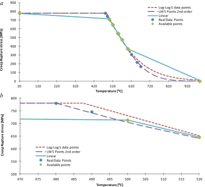
temperatures. The other two methods instead are able to provide much more accurate rupture data, and the Larson Miller approach is the one which leads to the most precise prediction. Figure 1b presents a closer view for temperatures between 480⁰C and 520⁰C. It can be seen clearly that the Larson-Miller approach is still the best option due to its capability of providing an accurate prediction; instead linear and logarithmic approaches respectively underestimate and overestimate the real experimental rupture stress. For each method the maximum and minimum temperatures are imposed. The maximum allowable working temperature is a material constant, and is an upper bound limit for the simulation. The minimum creep temperature is a material constant too, and depends on the rupture time. All the methods described in this section are implemented in the solution process through a FORTRAN subroutine called by the LMM creep rupture analysis via Abaqus user subroutine UMAT (Hibbitt et al., 2012), where the LM method is the default method to calculate the creep rupture stress, but the user is allowed to use other two schemes as well during the analysis.

4.

Holed plate

4.1

Finite element model for the holed plate example

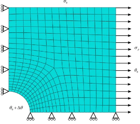
The first example analysed in this paper is a square holed plate subjected to a constant mechanical load and a cycling thermal load. A quarter of the plate is modelled due to the symmetry condition (Figure 2). The mesh used is composed by 642 20-node solid isoparametric elements, with reduced

integration scheme. The following geometric ratios are used in this study, D 0.2

L  where D is the hole

diameter and L the length of the plate, and t 0.05

L  where t is the plate thickness. In order to benchmark the new approach the same material properties used by (Chen et al., 2003) are considered. The material has a Young’s modulusE208 GPa, Poisson’s ratio



0.3and a constant yield stress_y 360 MPa.

A reference uniaxial tensile load _p360 MPais applied on the external face surface, and plain conditions are applied to the two external faces. The reference thermal elastic stress field is generated by imposing a thermal gradient over the component. The coefficient of thermal expansion of the material is

_

_{1.25 10 } 5 _C1_{. In order to generate the appropriate temperature field a user defined} subroutine is used, *UTEMP within Abaqus (Hibbitt et al., 2012), where the temperature gradient of the holed plate is defined using the following equation:

0

5

ln( a) / ln(5) r

     (18)

points using the coordinates to calculate the appropriate distance r from the plate centre. In order to compare the results obtained by using the new methodology with the previous approach a table of creep rupture stresses are calculated using equations (1) and (2).

4.2

Results and discussion for the holed plate example

An initial investigation has been performed for a given creep rupture time corresponding to R=0.5. A fictional rupture stress data is obtained using equations (1) and (2). To determine which is the most robust interpolation/extrapolation method three creep rupture batches are adopted (Table 1). The first batch contains creep rupture stresses at low temperature (300⁰C to 340⁰C), the second one at high temperature (450⁰C to 480⁰C) and the last one contains both. A single creep rupture limit calculation

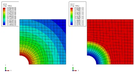
is performed, for the holed plate subjected to the reference thermal load and nil mechanical load. Direct comparison between linear interpolation method and LM method using different data batches is showed in Figure 3a. Using data batch-3 equal creep rupture limit multipliers are obtained (black line) for both methods. Instead using data batch-1, the solution provided by the linear interpolation is the less conservative. This outcome is due to the lower extrapolation accuracy of creep rupture stress over temperature. Instead the Larson-Miller approach is capable of interpolating and extrapolating a more precise creep rupture stress, which brings to a safer solution for data batch-1. If creep rupture stress data points provided are at high temperature (batch-2) the Larson Miller method produces very accurate creep rupture limit, contrary the linear interpolation method is over conservative. Figure 3b and Figure 3c show the converged revised yield stress calculated by using the linear interpolation method and LM method respectively. The creep rupture stress around the hole with the highest temperature calculated by the linear interpolation is about 90 MPa _{higher than the one predicted by} the Larson Miller approach. For these reasons the Larson-Miller parameter is considered to be the most appropriate approach leading to the accurate solution to the creep rupture stresses for the creep rupture analysis. Therefore, only the Larson-Miller parameter is considered in the rest of this paper.

leads to a lower revised yield stress, due to a lower value of R (i.e. longer allowable time to creep rupture).

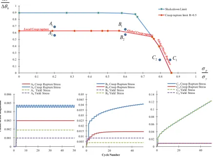
Figure 5 and Figure 6 show the creep effect due to load cases at points A and B, which are taken from the curve with R0.5 in Figure 4. When temperature is high enough creep is dominant (load point A), the revised yield stress is lower than the initial yield stress across a big component volume (Figure 5). Instead for load point B creep effect is highly reduced, and the reduction of the revised yield stress due to the high temperature is limited to a small volume around the hole (Figure 6). In order to confirm the obtained LMM creep rupture limit interaction curves in Figure 4, the creep rupture limit for R=0.5 is verified through a step-by-step analysis, considering the following cyclic load points, A1(0.2,0.65), A2(0.2,0.55), B1(0.6,0.65), B2(0.6,0.55), C1(0.85,0.2), C2(0.8,0.2) shown in

Figure 7, where cyclic load points A1, B1 and C1 are just outside the creep rupture limit curve for R=5,

and points A2, B2 and C2 are slightly below the creep rupture limit curve. In order to introduce the

creep rupture effect in the step-by-step analysis, the revised yield stress by the creep rupture stress is used to replace the yield stress. By comparing plastic strain histories for these cyclic load points (Figure 7) calculated by the step-by-step analysis, it can be seen that all the cyclic load points exhibit a shakedown behaviour when using the original yield stress of the material except for load point C1

which shows a ratchetting mechanism. Contrary when the creep rupture stress is considered, cyclic load points A1, B1 and C1 exhibit a non-shakedown behaviour, and cyclic load points A2, B2, C2 show

a shakedown mechanism. These significant mechanism changes between cyclic load points A1/B1/C1

and A2/B2/C2 indicate the applicability of the calculated creep rupture limit interaction curve for

R=0.5.

It can also been observed that the creep rupture limit interaction curve for R=0.5 exhibits three

distinct areas according to the applied constant mechanical load ranges, p 0.55 y



  , 0.55 0.75

p

y

 

 

and 0.75 p 0.85 y

 

  respectively. In the first load range local creep rupture behaviour is dominant,

instead a global creep rupture is present in the second one. The upper bound of the second mechanical load range represents the end of creep rupture effect on the component. In the third load range, where

0.75 p 0.85 y

 

  , the creep rupture does not take any effects due to the relatively low temperature.

The corresponding creep rupture limit curve is actually determined by a global ratchetting mechanism，and results are equal to the shakedown procedure. This threshold is not constant and varies with the defined rupture time. An extreme case is represented by the creep rupture limit for R=0.1 (Figure 4). In this case the revised yield stress is widely affected by the creep rupture and global ratchetting failure occurs only for temperature ratio below _0.1

0

 

 

typical failure mechanisms of holed plate corresponding to load points A1, B1 and C1, respectively, by

showing the plastic strain magnitude contours calculated by the step-by-step analysis using the revised yield stress with R=0.5. Local creep rupture occurs for load point A1 which affects strictly a local area

at high temperature, contrary the global creep rupture mechanism occurs for the cyclic load point B1

which affects a larger area across the thickness. For the cyclic load point C1, a global ratchetting

rather than the creep rupture becomes the failure mechanism, which is totally driven by the larger mechanical load and lower temperature.

5.

Two-pipe structure

5.1

Finite element model for the two-pipe structure

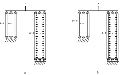
In the second example, the component is composed of two pipes with different lengths, which was originally created by (Abdalla et al., 2007) as a one dimensional problem made by two bars. Later (Martin and Rice, 2009) modified it by replacing the bars by pipes, and an internal pressure to the longer pipe was introduced. Both pipes were subjected to an axial force F and the longer one having a cycling temperature. This example was also adopted by (Lytwyn et al., 2015) to predict ratchet limit and it is useful to investigate different failure mechanisms. This paper further extends the example by cycling the temperature over each of the two pipes and considering creep rupture, as shown in Figure 9. Two thermal load cases are considered in this study; in case (a) the shorter pipe is at constant uniform temperature of 0⁰C and the longer one has a cycling uniform temperature between 0⁰C and the operating one. Contrary in case (b) the shorter pipe is subjected to that cyclic temperature and the longer pipe is set to constant uniform temperature of 0⁰C. In addition to this thermal load, the two-pipe structure is also subjected to an axial force F, given in Newton [N], and an internal pressure P given in [MPa] is applied on the longer pipe, a fixed force over pressure ratio of F/P=10 is considered. This ratio was adopted by (Lytwyn et al., 2015), demonstrating how it affects the ratchet limit. The ratio adopted here is considered to be the worst case scenario due to the severity of hoop stress comparing with the axial force. Despite the simple geometry, such an example is complex in terms of failure mechanisms and it is an ideal example to investigate the effect of creep rupture.

The entire model is composed of 1460 20-node solid isoparametric elements, with reduced integration scheme. The geometric dimensions adopted are given in Table 2. The two pipes have one end constrained in the axial direction and plane condition is applied to the other end allowing the two pipes to deform together. The material adopted is Nimonic 80A which has a Young’s modulus of

219

rupture stress. Hence the temperature dependent yield stress of material is used and it is reported in Table 3, as well as the temperature dependent creep rupture stresses for different times to rupture shown in Table 4. The creep rupture data of Nimonic 80A steel shown in Table 4 are obtained using the LM extrapolation procedure for 300 khrs of time to rupture and also 200 khrs when temperature is greater than 570⁰C.

5.2

Results and discussions for the two-pipe structure

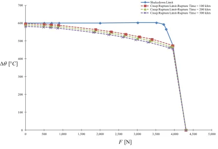
Both the shakedown limit and creep rupture limit interaction curves for different times to rupture for the two-pipe structure subjected to thermal load case (a) are obtained by the proposed method and shown in Figure 10. Axial force F is given in Newton [N], and the cyclic temperature range  in degree Celsius [⁰C]. The blue line represents the shakedown limit calculated using the original yield

stress of the material. Instead the dashed lines represent the creep rupture limits for rupture time of 100, 200 and 300 khrs, respectively.

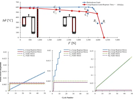
The creep rupture limit for a given rupture time of 100 khrs under cyclic thermal load case (a) (Figure 11) is verified by a series of step-by-step analyses, considering three cyclic load points just outside the creep rupture limits C1(2000,570), C3(3500,520), B1(4200,300) and three inside

C2(2000,540), C4(3500,490), B2(4000,300) as shown in Figure 11. In order to confirm the LMM creep

rupture limit for a given rupture time of 100 khrs by the step-by-step analysis, both the original yield stress and the revised yield stress (determined by the minimum of the creep rupture stress and the original yield stress of material) are adopted. By comparing plastic strain histories for these cyclic load points (Figure 7) calculated by the step-by-step analysis, it can be seen that all cyclic load points exhibit shakedown behaviour when adopting the original yield stress except for load point B1, which

shows a ratchetting mechanism. Instead considering the revised yield stress, cyclic load points C1, C3

and B1 show a non-shakedown behaviour (Figure 11), the cyclic load points C2, C4 and B2 which are

just inside the creep rupture limit curve show a shakedown behaviour. These significant mechanism changes between cyclic load points C1/C3/B1 and C2/C4/B2 confirm the accuracy of the calculated

creep rupture limit interaction curve for a given rupture time of 100 khrs. As for the holed plate problem, in this example creep effect also depends on the operating temperature, and for temperatures below 480⁰C creep does not occurs (Table 4). For this reason both cyclic load points B1 and B2 with a

temperatures below 480⁰C have identical plastic behaviour using either the yield stress or the revised

yield stress.

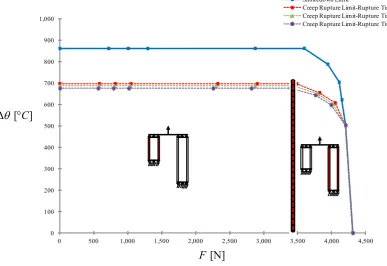
which is however still capable of bearing higher load under such a loading conditions comparing with the shorter pipe. For this reason creep does not affect the plastic behaviour of the shorter pipe significantly for low axial forces and internal pressures, which makes the creep rupture limit close to the shakedown limit. Instead for higher axial forces and internal pressures, the failure mechanism switches to the longer pipe (highlighted in red), and the difference between the shakedown and creep rupture limits is much more significant. In order to further investigate the effect of different high temperature condition on the creep rupture, the cyclic thermal load case (b) is also calculated the proposed method, and the corresponding shakedown and creep rupture limit interaction curves for different allowable times to creep rupture are presented in Figure 12. In this case failure occurs in the shorter pipe (highlighted in red) for an axial force up to 3500N, where the failure of the shorter pipe is dominated by the creep rupture due to the applied high temperature on it. As expected, comparing with the shakedown limit, the applied cyclic thermal load on the shorter pipe causes a significant reduction in the creep rupture limits of a two-pipe structure. Instead when axial force is higher than 3500N and temperature is above 500⁰C failure initiates in the longer pipe due to the larger internal pressure on it.

6.

Conclusions

This paper presents a robust but accurate method for creep rupture stress calculation based on limited creep rupture experimental data in the creep rupture limit assessment, which is developed within the Linear Matching Method framework. Three distinct approaches including linear interpolation, polynomial interpolation and Larson Miller parameter are considered for interpolation and extrapolation of creep rupture stresses. It has been identified by an initial investigation using fictional rupture stress data that the LM approach is the most robust and reliable in interpolating and extrapolating creep rupture stress among these three methods, especially when fewer rupture stress experimental data points are available.

The numerical example of a 3D holed plate is used for benchmarking purposes. The creep rupture limits obtained by the propose approach match with the results from previously published work. It can also been observed that the creep rupture limit interaction curve exhibits three distinct mechanisms, depending on the magnitude of the applied constant mechanical load. The three observed mechanisms are local creep rupture, global creep rupture and global ratchetting mechanism.

A second numerical example investigates creep rupture limits of a two-pipe structure considering two loading cases. Both shakedown limit and creep rupture limits for different rupture times are calculated for these two loading cases, which show a remarkable distinction in the creep rupture limit interaction diagram. In the first case for an axial load up to 900N the failure starts from the shorter pipe due to a reverse plastic mechanism. For a higher axial load the failure is always located at the longer pipe exhibiting a global creep rupture mechanisms. In the second case where the cyclic thermal load is applied to the shorter pipe, the difference between shakedown limit and creep rupture limit is remarkable, and the failure mechanism is located at the shorter pipe for axial load up to 3500N. This example demonstrates how creep rupture can affect the same structure in different ways due to the different temperature load conditions.

The initial convergence problem due to the fluctuation of the revised yield stress and scaled temperature is solved by introducing a damping factor during the scaling process when a fluctuation of the creep rupture limit multiplier takes place. The further convergence study shows that with the proposed numerical scheme the oscillating behaviour is damped within the limited number of iterations and the creep rupture limit multiplier converges quickly. The accuracy of the obtained creep rupture limits is also verified by the detailed step-by-step analyses, which are further used to investigate the interaction between the different failure mechanisms.

Acknowledgements

References

Abdalla, H.F., Megahed, M.M., Younan, M.Y.A., 2007. A simplified technique for shakedown limit load determination. Nuclear Engineering and Design 237, 1231-1240.

Ainsworth, R., 2003. R5: Assessment procedure for the high temperature response of structures. British Energy Generation Ltd 3.

Burden, R.L., 2001. Numerical analysis. Pacific Grove, CA : Brooks/Cole.

Chaboche, J., 1984. Anisotropic creep damage in the framework of continuum damage mechanics. Nuclear Engineering and Design 79, 309-319.

Chen, H.F., Engelhardt, M.J., Ponter, A.R.S., 2003. Linear matching method for creep rupture assessment. International Journal of Pressure Vessels and Piping 80, 213-220.

Chen, H.F., Ponter, A.R.S., Ainsworth, R.A., 2006. The linear matching method applied to the high temperature life integrity of structures. Part 1. Assessments involving constant residual stress fields. International Journal of Pressure Vessels and Piping 83, 123-135.

Dyson, B., 2000. Use of CDM in materials modeling and component creep life prediction. Journal of pressure vessel technology 122, 281-296.

Hibbitt, H., Karlsson, B., Sorensen, P., 2012. ABAQUS theory manual, version 6.12. Pawtucket, Rhode Island, USA.

Hyde, T., Xia, L., Becker, A., 1996. Prediction of creep failure in aeroengine materials under multi-axial stress states. International journal of mechanical sciences 38, 385-403.

Kachanov, L.M., 1999. Rupture time under creep conditions. International journal of fracture 97, 11-18.

Koiter, W.T., 1960. General theorems for elastic-plastic solids. North-Holland Amsterdam.

Larson, F.R., Miller, J., 1952. A Time-Temperature Relationship for Rupture and Creep Stresses. Trans. ASME July, 765-775.

Liu, Y., Murakami, S., 1998. Damage localization of conventional creep damage models and proposition of a new model for creep damage analysis. JSME international journal. Series A, Solid mechanics and material engineering 41, 57-65.

Lytwyn, M., Chen, H., Martin, M., Lytwyn, M., Chen, H., Martin, M., 2015. Comparison of the linear matching method to Rolls Royce's hierarchical finite element framework for ratchet limit analysis. International Journal of Pressure Vessels and Piping 125, 13-22.

Manson, S.S., Haferd, A.M., 1953. A Linear time-temperature relation for extrapolation of creep and stress - rupture data, Other Information: Orig. Receipt Date: 31-DEC-53. Lewis Flight Propulsion Lab., NACA, p. Medium: X; Size: Pages: 49.

Martin, M., Rice, D., 2009. A hybrid procedure for ratchet boundary prediction, ASME 2009 Pressure Vessels and Piping Conference. American Society of Mechanical Engineers, pp. 81-88.

Mendelson, A., Roberts Jr, E., Manson, S., 1965. Optimization of Time-Temperature Parameters for Creep and Stress Rupture, with Application to Data from German Cooperative Long-Time Creep Program. DTIC Document.

Pink, E., 1994. Physical significance and reliability of Larson–Miller and Manson–Haferd parameters. Materials science and technology 10, 340-346.

Ponter, A.R., Fuschi, P., Engelhardt, M., 2000. Limit analysis for a general class of yield conditions. European Journal of Mechanics-A/Solids 19, 401-421.

Ponter, A.R.S., Engelhardt, M., 2000. Shakedown limits for a general yield condition: implementation and application for a Von Mises yield condition. European Journal of Mechanics - A/Solids 19, 423-445.

Rabotnov, I.N., 1969. Creep problems in structural members. By Yu. N. Rabotnov. Translated from the Russian by Transcripta Service Ltd., London. English translation edited by F.A. Leckie. North-Holland Pub. Co, Amsterdam, London.

List of figures

500 550 600 650 700 750 800

470 475 480 485 490 495 500 505 510 515 520

C re e p R upt ur e s tr e ss [ M P a] Temperature [⁰C]

Log-Log 5 data points LM 5 Points 2nd order Linear

Real Data Points Available points 0 100 200 300 400 500 600 700 800 900

20 120 220 320 420 520 620 720 820 920

C re e p R u p tu re s tr e ss [ M P a] Temperature [⁰C]

Log-Log 5 data points LM 5 Points 2nd order Linear

Real Data Points Available points

a

b

[image:17.595.85.498.126.502.2]

0



 



0



0



p

[image:18.595.70.520.80.479.2]



0.45 0.5 0.55 0.6 0.65 0.7 0.75

5 15 25 35 45 55 65

C

re

ep

R

up

tu

re

m

ul

ti

pl

ie

r

Iterations

Solution using Batch-3 data points LM Interpolation using Batch-1 data points Linear Interpolation using Batch-1 data points LM Interpolation using Batch-2 data points Linear Interpolation using Batch-2 data points a

b c

Figure 3 a) Convergence of creep rupture limit for different interpolation techniques, b) and c) Revised yield stress contour obtained by linear interpolation and Larson Miller method [MPa],

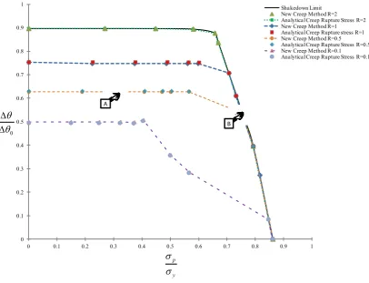
[image:19.595.76.522.75.412.2]

0 0.1 0.2 0.3 0.4 0.5 0.6 0.7 0.8 0.9 1

0 0.1 0.2 0.3 0.4 0.5 0.6 0.7 0.8 0.9 1 Shakedown Limit New Creep Method R=2 Analytical Creep Rupture Stress R=2 New Creep Method R=1 Analytical Creep Rupture stress R=1 New Creep Method R=0.5 Analytical Creep Rupture Stress R=0.5 New Creep Method R=0.1 Analytical Creep Rupture Stress R=0.1

A

B

0

 

 

p

y

[image:20.595.76.483.75.386.2]

 

[image:21.595.72.523.72.325.2]

Figure 5 Effect of temperature (left contour) on the revised yield stress (right contour) for load point A (Figure 4)

[image:21.595.71.523.392.652.2]

0 0.1 0.2 0.3 0.4 0.5 0.6 0.7 0.8 0.9 1

0 0.1 0.2 0.3 0.4 0.5 0.6 0.7 0.8 0.9 1

Shakedown Limit Creep rupture limit R=0.5 0     p y   1 A 2 A 1 B 2 B 2

C C₁

0 0.001 0.002 0.003 0.004 0.005 0.006

0 10 20 30 40 50

P la st ic st ra in m ag ni tu de

A₂Creep Rupture Stress A₁Creep Rupture Stress A₁Yield Stress A₂Yield Stress

0 0.005 0.01 0.015 0.02 0.025 0.03 0.035 0.04 0.045 0.05

0 20 40

B₁Creep Rupture Stress B₂Creep Rupture Stress B₁Yield Stress B₂Yield Stress

0 0.02 0.04 0.06 0.08 0.1 0.12 0.14

0 20 40

C₁Creep Rupture Stress C₂Creep Rupture Stress C₁Yield Stress C₂Yield Stress

[image:22.595.81.519.84.407.2]

Cycle Number Local Creep rupture

Figure 7 Verification of the LMM creep rupture limit for holed plate by comparing plastic strain histories from detailed step-by-step analyses.

1

A B₁ C1

Local Creep rupture Global Creep rupture Global Plastic rupture

[image:22.595.80.520.483.669.2]

F

θ = 0

∆θ +θ P

P = 0

F

θ = 0 ∆θ +θ

P

P = 0

[image:23.595.88.513.70.334.2]

a b

Figure 9 Finite element model of the two-pipe structure subjected to an axial force F and an internal pressure P on the longer pipe, with a fixed force over pressure ratio of F/P=10, as well as a thermal

[ ]C

  

[N]

F 0

100 200 300 400 500 600 700

0 500 1,000 1,500 2,000 2,500 3,000 3,500 4,000 4,500 5,000 Shakedown Limit

[image:24.595.74.514.72.373.2]

Creep Rupture Limit-Rupture Time = 100 khrs Creep Rupture Limit-Rupture Time = 200 khrs Creep Rupture Limit-Rupture Time = 300 khrs

0 100 200 300 400 500 600 700

0 500 1,000 1,500 2,000 2,500 3,000 3,500 4,000 4,500 5,000 Shakedown Limit

Creep Rupture Limit-Rupture Time =100 Khrs

1 B 2 B 1 1 C 2

C C3

4 C

[ ]C    [N] F 0 0.05 0.1 0.15 0.2 0.25

0 10 20 30 40 50 B₁Creep Rupture Stress B₂Creep Rupture Stress B₁Yield Stress B₂Yield Stress

0 0.005 0.01 0.015 0.02 0.025 0.03

0 10 20 30 40 50

P la st ic st ra in m ag ni tu de

C₁Creep Rupture Stress C₂Creep Rupture Stress C₁Yield Stress C₂Yield Stress

0 0.005 0.01 0.015 0.02

0 10 20 30 40 50 C₃Creep Rupture Stress C₄Creep Rupture Stress C₃Yield Stress C₄Yield Stress

Cycle Number

[image:25.595.79.515.69.393.2]

100 khrs

0 100 200 300 400 500 600 700 800 900 1,000

0 500 1,000 1,500 2,000 2,500 3,000 3,500 4,000 4,500 Shakedown Limit

Creep Rupture Limit-Rupture Time = 100 khrs Creep Rupture Limit-Rupture Time = 200 khrs Creep Rupture Limit-Rupture Time = 300 khrs

[ ]C

  

[N]

[image:26.595.86.474.79.345.2]

F

0.85 0.9 0.95 1 1.05 1.1 1.15 1.2

1 6 11 16

C re ep r up tu re m ul ti pl ie r Iterations

Creep Rupture Multiplier

0 100 200 300 400 500 600 700 0 100 200 300 400 500 600

1 6 11 16

T em pe ra tu re [ ⁰ C ] R ev is ed Y ie ld S tr es s [M Pa ] Iterations

Revised Yield Stress Temperature

a

b

[image:27.595.91.503.74.526.2]

[image:28.595.105.490.171.383.2]

List of tables

Table 1 Creep rupture data of fictional steel

Temperature [⁰C] Creep rupture stress [MPa] for R = 0.5

Batch-3

Batch-1

300 360

310 327

320 300

330 276

340 257

Batch-2

450 144

460 138

470 133

[image:28.595.202.396.471.591.2]

480 128

Table 2 Two-pipe structure dimensions

Property Pipe 1 Pipe 2

Length 100 200

Outside radius (mm) 2.68 3.22

Inside radius (mm) 2.00 2.00

Table 3 Temperature dependent yield stress of Nimonic 80A steel alloy

y

 (T) [MPa] _{780 725 700 455 50}

[image:28.595.66.530.680.745.2]

[image:29.595.67.528.104.338.2]

Table 4 Creep rupture data of Nimonic 80A steel at different rupture times, [*] extrapolated data

Temperature [⁰C] Creep rupture stress 100 khrs [MPa]

Creep rupture stress 200 khrs [MPa]

Creep rupture stress 300 khrs [MPa]

480 779 742 693*

490 746 709 662*

500 713 675 628*

510 680 640 592*

520 646 606 555*

570 475 412* 366*

600 372 312* 264*

620 306 253* 206*

650 217 177* 135*