Maintenance scheduling for multicomponent systems with hidden failures

1

Maintenance scheduling for multi-component systems with hidden failures

Bin Liu a,_{*, Ruey-Huei Yeh} b_{, Min Xie} a,c_{, Fellow, IEEE, Way Kuo} a_{, Fellow, IEEE}

a _{Department of Systems Engineering and Engineering Management,}

City University of Hong Kong, Kowloon, Hong Kong

b _{Department of Industrial Management,}

National Taiwan University of Science and Technology, Taipei, Taiwan

c _{Shenzhen Research Institute, City University of Hong Kong, Shenzhen, China}

* Corresponding author. Email: [email protected]

Abstract

This paper develops a maintenance policy for a multi-component system subject to hidden

failures. Components of the system are assumed to suffer from hidden failures, which can only

be detected at inspection. The objective of the maintenance policy is to determine the inspection

intervals for each component such that the long-run cost rate is minimized. Due to the

dependence among components, an exact optimal solution is difficult to obtain. Concerned with

the intractability of the problem, a heuristic method named “base interval approach” is adopted

to reduce the computational complexity. Performance of the base interval approach is analyzed

and the result shows that the proposed policy can approximate the optimal policy within a small

factor. Two numerical examples are presented to illustrate the effectiveness of the policy.

Key words: Hidden failure, multi-component system, maintenance optimization,

inspection-replacement policy, base interval approach

1. Introduction

With the integration of technologies, modern systems are often complex systems consisting of

2

neglected when making maintenance decisions. Optimal maintenance strategy for an individual

component may not necessarily remain optimal for a system consisting of multiple dependent

components. If no dependence exists among components, maintenance strategy for

multi-component systems is identical with that for a single-multi-component systems (Wang, 2002).

Dependency among components however brings a lot of challenges to multi-component

maintenance optimization (Gustavsson et al, 2014; Phan & Zhu, 2015; Liu et al, 2015).

In the literature, two strategies have been widely used to deal with the multi-component

maintenance issue, namely, group maintenance and opportunistic maintenance (Nicolai &

Dekker, 2008). Group maintenance implies that multiple components are replaced in groups at

predetermined times (Xiao et al, 2016). Vu et al (2014) proposed a dynamic group maintenance

strategy for multi-component systems. Gao et al (2015) proposed a dynamic interval

maintenance policy, which is more effective in reducing unnecessary maintenance actions

compared with periodic preventive maintenance. Opportunistic maintenance occurs in the case

that components are maintained when a maintenance opportunity arises, e.g., unexpected system

shutdown. Pandey et al (2016) proposed a preventive maintenance scheduling model where

maintenance actions are implemented during system breakdown. Recently, more advanced

maintenance policies (e.g., condition-based maintenance) have been applied for multi-component

systems (Camci, 2009). Liu et al (2014) proposed a value-based maintenance policy for

multi-component systems with degrading multi-components. In the work of Tian & Liao (2011), a condition

based maintenance strategy with proportional hazards model was developed for multi-component

systems.

Although numerous maintenance policies for multi-component systems have been proposed in

literature, most of the models focus on catastrophic or sudden failures (failures that are

self-announcing). However, in many cases, failures are not self-announcing, that a failure remains

dormant before being exposed by inspection techniques or other system disturbances. This type

of failure is referred to as hidden failure or soft failure (Ye et al, 2014; Ye & Xie, 2015; Wang et

al, 2016). Hidden failure itself does not lead to system breakdown, but the existence of hidden

failure may cause performance loss during system operation. Hidden failure is very common in

modern systems, particularly in stand-by redundant systems and protection systems (Xiao & Ye,

3

component outages and even spread power system disturbances. Cheng et al (2013) pointed out

that hidden failure of relay protection system is the main contributor of cascading failures and

blackouts.

A common practice to deal with hidden failure is to implement an inspection policy to detect

the existence of hidden failures (Lam & Banjevic, 2015). Based on the interval between two

consecutive inspections, inspection policy can be classified into two types: periodic inspection

and sequential inspection (non-periodic). A common practice in industry is to implement

periodic inspection at constant intervals, due to its feasibility and applicability. In literature, there

exist plentiful research works on dealing with hidden failures. Wang & Pham (2011) investigated

a multi-objective maintenance optimization for systems with dependent competing risks of

degradation wear and random shocks. Ahmadi & Kumar (2011) studied cost based risk of system

with hidden failures, where the optimal inspection and restoration intervals are determined based

on the cost criterion. He et al (2015) considered an imperfect inspection policy for system subject

to hidden failures, in which the interval of imperfect inspection interval and the number of

imperfect inspections are determined so as to achieve an optimal maintenance strategy. Liu et al

(2017) proposed a condition-based maintenance policy for a system with age- and

state-dependent operating cost, where the side effect of degradation is investigated.

Although numerous studies have accommodated to hidden failures, most focus on

maintenance/inspection policy for a single-component system. However, modern systems are

usually subject to multiple hidden failures. For example, a protection system contains multiple

components such as transducer and relays, and hidden failure may occur in any of the

constituents. It is thus necessary to investigate hidden failure in a multi-component context. Yet

few efforts have been devoted to multiple-component maintenance policy with hidden failures.

Zhu et al (2016) established a multi-level maintenance model for a system with multiple failure

modes. Taghipour & Banjevic (2011) developed a periodic inspection policy for a repairable

system, where the components are subject to hidden failures. In that work, the optimal inspection

interval was applied for all the components. Huynh et al (2014) proposed a multi-level

maintenance policy, where the system was intervened at both the component and the system

level. Long-run cost rate was minimized by jointly optimizing the inspection interval and

4

components are inspected simultaneously or a common metric is used for all the components.

However, as the components in the system vary in degradation process and maintenance cost, it

is more desirable to apply different maintenance metrics for heterogeneous components.

In this paper, we aim to develop a maintenance policy for a multi-component system subject to

hidden failures. The objective of this study is to determine the inspection intervals for each

component such that the long-run cost rate is minimized. Here, we focus on the effect of

economic dependence since economic dependence is the most common interaction in a

multi-component system. With respect to the maintenance optimization of the multi-multi-component system,

the difficulty lies in the computational complexity. Actually, optimization of multi-component

maintenance scheduling with economic dependence has been proven to be an NP-complete

problem (Levi et al, 2014). To deal with the intractability of this problem, we adopt a heuristic

method named “base interval approach” on the basis of Laggoune et al (2009) and Hopp & Kuo

(1998). The base interval approach reschedules the inspection interval of each component as an

integer multiplier of a base interval, so as to share the common downtime cost and reduce

maintenance cost. In addition, we investigate the performance of the base interval approach,

where the effectiveness of proposed approach is demonstrated both analytically and numerically.

The remainder of this paper is organized as follows. Section 2 describes the problem and

formulates the maintenance model. Maintenance policy using base interval approach is proposed

in Section 3 and performance analysis of the approach is presented in Section 4. Numerical

examples are presented in Section 5. Finally, concluding remarks and future discussions are

given in Section 6.

Notations

I

C Common downtime cost due to inspection

i d

c Downtime cost per unit time of component i

i I

c Inspection cost of component i

i r

c Replacement cost of component i

i d

5

( )

G Long-run cost rate of the system

( )

i

G Long-run cost rate of component i, without considering the common cost

i

k Integer multiplier, indicating the rescheduled inspection interval of component i

i=1,2,…,n Component index

d

N (t) Number of system shutdown due to inspection till time t

i I

N (t) Number of inspections of component i till time t

n Number of components

( )

i

R t Reliability function of component i at time t

i

S Length of a renewal cycle of component i

i

T Time to failure of component i

i

 Mean time to failure of component i

 Base inspection interval

i

 Inspection interval of component i

2. Maintenance model formulation

2.1 General description and assumptions

Consider a he system consisting of multiple non-identical components. Each component

suffers an underlying deteriorating process and fails randomly according to specific lifetime

distribution. The components are non-repairable; if a component is found to have failed, it has to

be replaced by a new one. Note that although the components are restored to the

‘as-good-as-new’ condition after replacement, the whole system is not perfectly maintained except that all the

components are replaced simultaneously.

An inspection-replacement policy is implemented on each component. The components are

inspected at periodic intervals with the individual inspection cost c_Ii. When an inspection is

performed on a component, the whole system has to be shut down, which incurs a common

downtime cost CI. The common cost due to inspection can be shared when multiple inspections

are carried out simultaneously. Without loss of generality, it is assumed that the set-up cost and

6

detected at inspection, the associated component is replaced immediately. During the period of

hidden failures, additional cost is incurred due to performance loss of the component, denoted as

i d c .

In terms of constructing a realistic model, the following assumptions are made:

1. Failure of a component is not self-announcing; it can only be revealed at inspection.

2. Inspection can be implemented on each component; inspection on a component is perfect.

When a failure occurs, it can always be discovered at the next inspection.

3. A common cost is incurred at each inspection time, which can be shared when multiple

inspections are carried out simultaneously. The assumption of constant common cost is

reasonable when multiple maintenance crews are available to inspect the components.

4. Only economic dependence exists between components. Structural dependence and

stochastic dependence are not considered.

5. The component is non-reparable; only replacement is applicable when a failure is

revealed on a component. Replacement is instantaneous and restores the component to

the ‘as-good-as-new’ condition.

6. Deterioration of a component remains unchanged during inspection.

2.2 Cost model

Consider a system consisting of n heterogeneous components. Let _i, i=1,2,…,n, be the

inspection intervals for component i. The cost items can be divided into two categories. One is

the component-level cost, which is related to specific component and varies for different

components. The other category is the system-level cost, which is irrelevant to the component

and can be shared by multiple maintenance actions.

Component-level cost: component inspection cost ci_I , component replacement cost c_ri ,

performance loss (due to hidden failures of components) cost per unit time i

d c .

System-level cost: common downtime cost due to inspection C_I.

For an individual component i, one has to pay the associated cost at time t,





( ; ) i i( ; ) i i( ; ) i i( ; )

i i I I I i r r i d d i

7

where i is the inspection interval of component i, Hi is the total cost of component i

incorporating the common downtime cost, i

I

N is the cumulative number of inspections for

component i, N t_ri( ; )_i is the cumulative number of replacement for component i, and i( ; )

d i T t

is the cumulative downtime of component i. However, for a multi-component system, there may

be cases that the common cost has already been shared by other components (e.g., due to

inspection of other components). If this happens all the time, then we can neglect the common

cost C_I. In such cases, the corresponding cost of a component at time t is

H t_i( ; )_i c N ti_{I I}i( ; )_i c N t_ri _ri( ; )_i c T t_di _di( ; )_i (2) As shown in Eq (1) and (2), the total maintenance cost can be reduced if multiple components

are inspected simultaneously. As the common cost can be shared when performing inspections

together, it is of interest to schedule inspections in groups so that multiple inspections can be

implemented at one scheduled inspection time. However, on the other hand, rescheduling the

inspection time incurs additional cost. As we will see in the following sections, each component

has its optimal inspection interval so as to minimize the individual long-run cost rate. If the

inspection interval is postponed or advanced in order to share common downtime cost C_I ,

additional cost is incurred compared with the minimal cost obtained at the optimal inspection

interval. We have to consider this tradeoff when grouping multiple components to share the

common downtime cost. An optimal policy should balance the potential benefit and the

associated additional cost.

If the components are inspected with intervals  ₁, ₂,...,_n, the long-run cost rate of the system

is expressed as

1 2

1 2

( , ,..., ) 1

( ; ) ( ; , ,..., )

= lim

n

n

i i d n I

i t

H t N t C

G

t

        





(3)

where N td( )is the number of system shutdown till time t. Obtaining an optimal solution of Eq (3)

is difficult due to the economic dependence among components. Indeed, optimization of Eq (3)

is an NP-hard problem as the number of combinations increases exponentially with the number

8

that can provide a near optimal solution. In the following, we adopt base interval approach to

deal with the computational complexity.

3. Maintenance policy with base interval approach

Base interval approach was initially proposed to solve the joint replacement issue of an aircraft

engine (Hopp and Kuo, 1998). It was inspired by the power-of-two replenishment policy in

inventory management (Jackson et al, 1985). Laggoune et al (2009) applied the base interval

approach in opportunistic maintenance for a continuously operating system. The basic idea of

base interval approach is to find a base interval  such that the common cost is charged at every

 time units and the component is inspected at some integer multipliers of the base interval, k_i .

In other words, at least one component is inspected in each multiple of  . Under this scenario,

our objective is to find the optimal base interval  and a set of integers





the long-run cost rate of the system is minimized. The optimization problem is formulated into

1 2

1

, , ,...,

( ; ) min lim

. . 0, , 1, 2,...,

n

n

i i

i I

k k k t

i H t k

C t

s t k Z i n



  

 





   



(4)

where Z denotes the set of positive integers.

A natural way to calculate the long-run cost rate is to use the renewal cycle theorem and

compute the expected cost rate in a renewal cycle of the system (Zhang et al, 2015). However, in

the present case, a renewal cycle occurs only when all the components are replaced

simultaneously, which takes extremely long time or even never occurs. Hence, it is difficult or

even impossible to compute the long-run cost rate function based on renewal cycle theorem.

However, by observing the cost structure of Eq (4), we can decompose the objective function

from system level into component level, and then apply the renewal cycle theorem individually.

As we can see, the objective function contains two terms: the first term,

1

lim n _i( ; _i ) / i

t



9

component. By taking advantage of the cost structure, we proceed to study the individual optimal

maintenance policy so as to reduce the computational complexity.

3.1 Individual optimal maintenance policy

In this section, we formulate a cost model for an individual component and obtain the optimal

individual inspection interval. When a component is replaced at inspection, the component is

restored to the ‘as-good-as-new’ state, which constitutes a renewal cycle (Liu et al, 2016).

According to the renewal cycle theorem, the individual long-run cost rate is given as

( ; ) [ ( )]

( ) lim

[ ]

i i i i

i i _t

i

H t E H S

G

t E S

 



 

where S_i is the length of a renewal cycle of component i. Denote Ti as the failure time of

component i. Let R t_i( )be the reliability function of the component and ( )

i

T

F t be the cumulative

density function (cdf) of the failure time. For notational simplicity, we denote the number of

inspection in a renewal cycle and the downtime in a renewal cycle for component i as N_Ii and T_di,

instead of N S_Ii( )_i and T S_di( )_i . N_Ii is related to the failure time and the inspection interval, which

is denoted as N_Ii  _T_i/_i_ (Badia et al, 2001). The expectation of i

I

N is calculated as













1

1 0

[ ] ( 1)

( ) ( 1) ( )

i i

i

I i i i

j

T i T i i i

j j

E N jP j T j

j F j F j R j

 

  

 

 

 

   

   







The length of a renewal cycle depends on i

I

N and _i, according to the assumption that

replacement can only be carried out at inspection. We have S_i N_Ii_i and the associated

expectation E S[ ]_i _i



between occurrence of a failure and replacement (end of a renewal cycle), T_di N_Ii_iT_i. The

expectation is

0

[ _di] _{i i}( _i) _i

j

E T 



component. Based on the above discussion, the expected cost in a renewal cycle can be obtained

10

0 0

[ _i ( )]_i i_{d i i}( _i) _{i r}i i_{I i}( _i)

j j

E H S c  R j  c c R j

 

 

 

 _  _ 







The long-run cost rate is then formulated as

0 0 ( ) [ ( )] ( ) [ ] ( )

i i i

d i r I i i

j i

i i

i i d

i

i i i

j

c c c R j

E H S

G c E S R j               





Proposition 1. If c_di_i ci_r ci_I, there exists optimal inspection interval _i* such that the

long-run cost rate reaches its minimum. Otherwise, *

i

  . Mathematically,





*

*

: ( ) / 0 , if

, otherwise

i i i

i i i i i d i r I

i

dG d c c c

               

The detailed proof is shown in the Appendix.

Proposition 1 implies that if c_di_i c_ri ci_I, it is beneficial to inspect the system with the

inspection interval *

i

 ; otherwise, inspection is unprofitable and we should resort to other

maintenance policies. In this study, we consider the case that the condition of ci_d_i c_ri ci_I can

always be satisfied; otherwise, the maintenance problem is trivial and makes no sense. This

assumption is plausible as the downtime cost is relatively high for modern complex systems and

the inspection cost is becoming lower with the development of inspection techniques. The

condition in Proposition 1 is equivalent to _i (c_Ii c_ri) /c_di , which implies that whether an

optimal inspection interval exists or not can be easily judged by comparing the MTTF of a

component with a constant value.

3.2 Selection of k_i

Based on the previous discussions, we can sketch G_i( )_i as shown in Fig 1. Since the system

is inspected at some integer multiples of the base interval  , the optimal ki should be either

*

/

i  

 

11 * * 0 0 * * * * * 0 0 * ( / ) ( / )

/ , if

/ ( / ) / ( / )

/ , otherwise

i i i i i i

d i r I i i d i r I i i

j j

i i

i i i i i i

j j

i

c c c R j c c c R j

k _{R j R j}

                                 _{         }             _{       }       









Therefore, once the base interval is given, the optimal inspection intervals for each component

can be easily obtained. The objective is reduce to find the optimal base interval *such that the

long-run cost rate of the system, ( )G , is minimized, i.e.,

* *

0 0

0 _{* * * *}

1 1

0 0

( / ) ( / )

min ( )

/ ( / ) / ( / )

i i i i i i

d i r I i i d i r I i i

n n j j i I d i i

i i i i i i

j j

c c c R j c c c R j

C

G c

R j R j

           _{           }        _{ }   _{         }               _{       }             













where the operator (xy)min( , )x y .

Fig 1 Sketch of G_i( )_i

Optimal solution of Eq (7) can be obtained by a simple search algorithm, described as follows:

1. Initialization: For each component, compute the individual optimal inspection interval

*

i

 ,i1, 2,...,n.

12

3. Determine k_i for each component, according to Eq (6).

4. Compute the value of G( ) according to Eq (7).

5. Increase  for a small increment, repeat step 3-4. Stop until  max





6. Output the minimal G*( ) and the associated *.

The time complexity of the algorithm is O n

 

as rolling horizon approach and brute-force search approach, the proposed base interval approach

shows the advantage of computational effectiveness.

4. Performance analysis

Now that we have described the base interval policy, we proceed to analyze the effectiveness

of the policy. A natural way to achieve this purpose is to compare the cost value obtained by our

approach with the optimum value. However, for the present case, the optimal solution is difficult

to obtain. Hence, instead, we demonstrate the effectiveness of our policy by comparing the upper

bound of our approach with the lower bound of the optimal solution.

4.1 Lower bound of the optimal solution

The idea of obtaining a lower bound is to allocate the maintenance cost of the whole system

on individual components. Let





to inspection, where l is the number index of system shutdown. Let tl

i

x be the action for

component i at time t_l, where

0, if no inspection is performed for component at

1, if inspection is performed for component at

l l

t i

l i t x

i t 

  

Let ( ) be the indicator function, where for any 0,

0, 0

( )

1, 0

if if

  

  

  _



With the notations defined above, we can transform the problem of minimizing system

long-run cost rate into finding the optimal tl*

i

13 1 1 ( ; ) min lim l tl i n n t

i i i I

i i

t x

H t x C

t            

 





It is straightforward to have (Atkins & Iyogun, 1987)

 

1 1

l l

n n

t t

i i i

i i x x       _   





where _i 0,  i 1, 2,...,n , and

1 1

n i i 



obtained as

 

 

i i i i I

i i

t

t n

i i i i I

t i

H t x C

t

H t x C

t                







For notational simplicity, denote





 

, lim

l

t

i i i i I

i i i t

H t x C

t         

so that





1 ,

n

i i i i  

 



single-unit cost items, with the common constraints



each inspection time, the individual inspection cost ci_I and common shutdown cost _iC_I are

charged; at the end of a renewal cycle of the component, the individual replacement cost c_ri and

component downtime cost c Ti_d _di are incurred. Therefore, for a fixed _i, _i





to the individual long-run cost rate of component i, with additional common downtime cost iCI

14

 









arg min ,

( )

arg min

( )

i

i

i i i i i

i i i

d i r I i I i i

j i

d

i i i

j

c c c C R j

c R j                       





Eq (10) implies that if _i 0 is given for component i, an optimal inspection interval  _i*

 

can be readily obtained. Let

 





*

, |

i i i

i i i  i i _{  }

   , the tightest lower bound becomes

 





Based on the above discussions, the optimization problem in Eq (8) is transformed into finding

optimal allocation (_iC_I) of the common downtime cost to each component so that the lower

bound reaches its maximum. In the work of Hopp & Kuo (1998), it was observed that the lower

bound increases when allocating higher percentages of the system intervention cost to

components with smaller replacement interval. Here, we follow the similar procedure and assign

higher proportion of the common cost to components that are inspected more frequently.

Without loss of generality, relabel the number of components according to their individual

optimal inspection intervals. Component with a smaller inspection interval is associated with a

smaller index. Assuming that the common downtime cost C_I is allocated to components

1, 2,..., , with the corresponding fraction _i, where

1 i 1

i





 



component i is  for i1, 2,..., and _i* for i  1,2,...,n. Then, the lower bound of the

system’s long-run cost rate is given as

*

1 1

( ) ( )

n I

i i i

i i

C

LB G G





 

   

 





15

Followed by the above discussions, we first analyze the upper bound of the base interval policy for an individual component, as shown in Lemma 1.

Lemma1. For an individual component, the base interval policy for component i is guaranteed

to have a cost at most





/

i i i

   times of the optimal solution.

The detailed proof is shown in the Appendix. Generally, the optimal individual inspection

interval _i* is much less than the MTTF of the component _i (as shown in the numerical

examples), which indicates that the proposed base interval policy can perform quite well

individually. Based on the individual analysis from Lemma 1, we can conclude the upper bound

of the system long-run cost rate, as shown in Proposition 2.

Proposition 2. The upper bound of the base interval policy is at most









sup  _i _i /_i:i1, 2,...,n times of the lower bound.

The detailed proof is shown in the Appendix. Proposition 2 indicates that the base interval

policy is guaranteed to approximate the optimal solution within a small factor.

For the problem of multi-component maintenance with hidden failures, the most intuitive

approaches are the individual inspection policy and common inspection policy (Taghipour &

Banjevic, 2011). It is interesting to compare the performance of the base interval approach and

the extant two approaches. Obviously, the base interval approach always outperforms the

common inspection policy. This is due to the fact that the base interval approach is actually a

generalization of the common inspection policy. For any determined base interval  , if all the ki

are set to 1, then the base interval approach is reduced to the common inspection policy.

On the other hand, the advantage of base interval approach over the individual inspection

policy highly depends on the common downtime cost C_I. If the common downtime cost is low,

the additional cost of rescheduling the inspection intervals may overwhelm the shared cost,

which implies the disadvantage of the base interval approach. This leads to another interesting

issue that under what condition the base interval approach outperforms the individual inspection

policy. In addition, for some components, the penalty cost due to rescheduling may exceed the

common downtime cost, though not usual in reality, then it would be optimal to remain the

16

intervals of other components are rescheduled. The proposed base interval approach can be

further improved by determining which components should be rescheduled and which should

remain unchanged.

5. Numerical examples

In this section, two examples are presented to illustrate the effectiveness of the base interval

approach. For the first example, we consider a 3-component system, where each component

follows an exponential lifetime distribution. In the second example, the proposed maintenance

policy is applied in a centrifugal compressor of a catalytic reforming unit.

5.1 An illustrative example with a 3-component system

A system consisting of three components is used to illustrate the base interval approach. The

components are assumed to follow an exponential lifetime distribution, with the reliability

function R t_i( )exp(_it), where _i is the failure rate of component i, i1, 2,3. At first, we

analyze the optimal inspection policy for an individual component. Based on the discussion in

Section 3.1, we have

0 [ ] ( ) 1 i i i i i

I i i

j

e

E N R j

e        



By substituting Eq (11) into Eq (5), long-run cost rate is expressed as

[ ( )]

( )

[ ] i i

i i

i d i i d

r I r

i

i i i i

i d

i i i

c c

c c c

E H S

G c

E S e

 



 

  

    (12)

The optimal inspection can be obtained by setting the derivative of to 0, i.e.,

2 2 ( 1) ( ) 0 i i i i

i d i i d

r i i I r

i

i i i

i i i

c c

c c c

G e                 _{ }   

 (13)

17

*

: ( 1) i i 0

i i

i d i i d

i i r i i I r

i i

c c

c c c e

  

 

     

 

_{ }  _  _   _  _

     

 , where

i

i i d

r I i

c

c c

  

The parameters of the failure rate and cost items are listed in Table 1. By use of numerical

methods, the individual optimal inspection interval is obtained as ₁* 1.19, ₂*1.39, ₃* 2.26,

and the corresponding optimal individual long-run cost rate is respectively *

1( ) 121.91

G   ,

*

2( ) 187.92

G   , G₃*( )₃ 202.4. In addition, we plot the variation of individual long-run cost

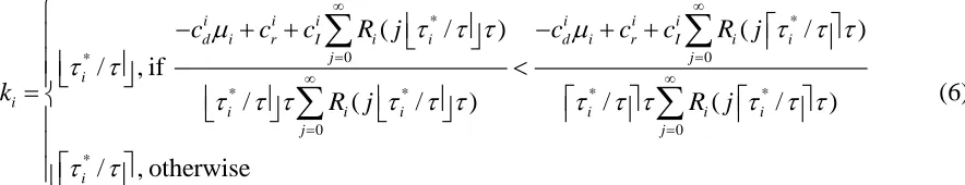
rate G_i (_i ) with respect to the individual inspection interval _i , as shown in Fig 2.

Table 1 Parameters of component-specific failure rate and cost items

Component Failure rate

i

 MTBFi

Replacement cost

i r c

Inspection cost

i I c

Downtime costc_di

1 0.02 50 200 70 5000

2 0.05 20 420 115 2500

3 0.1 10 640 150 750

Fig 2 Variation of G_i (_i )with _i

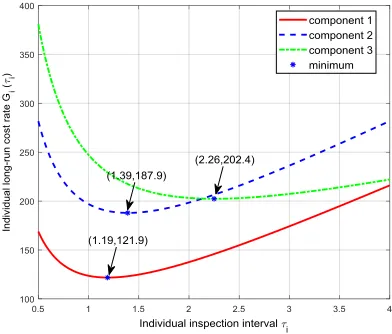
With regard to the whole system, the common downtime cost is set as C_I 60 . The

relationship between G( ) and  is given in Eq (7). Fig 3 shows how the long-run cost rate

( )

G changes with the base interval  . As we can see, when the base interval is  1.4, the

18

1 1

k  ,k₂ 1,k₃ 2. The result implies that based on the base interval approach, when we

inspect component 1 every k₁ 1.4 unit time, component 2 everyk₂ 1.4 unit time, and

component 3 every k3 2.8 unit time, we have the optimal maintenance policy. Table 2 shows

the comparison of the base interval approach, the individual inspection policy and the common

inspection policy (Taghipour & Banjevic, 2011). The result shows that the proposed base

interval approach dominates the other policies.

Fig 3 Variation of ( )G with respect to 

Table 2 Comparison of the rescheduled inspection policy, the individual inspection policy and common inspection policy

Component inspection interval ₁ 2 3 Cost rate

Individual inspection policy 1.19 1.39 2.26 692.2

Common inspection policy 1.69 1.69 1.69 562.9

19

In addition, Proposition 2 implies that the upper bound of the base interval policy is at most









sup  _i _i /_i:i1, 2,3 1.226 times of the lower bound. Here, the lower bound is

calculated as LB = 556.4. The long-run cost rate obtained by the base interval approach is

actually 1.005 times of the lower bound, which indicates that the base interval approach performs

quite effectively.

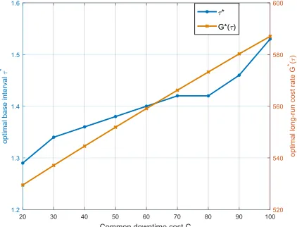
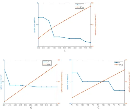
We are interested in the value of the common downtime cost C_I, since C_I characterizes the

economic dependence among components and affects the necessity of performing base interval

approach. Sensitivity analysis is carried out on CI to find out how CI influences the optimal

base interval and the optimal long-run cost rate. Fig 4 shows how the optimal inspection interval

*

 and the associated long-run cost rate G*( ) vary with different C_I . As can be observed,

*

( )

G  increases monotonically with C_I and * shows a non-decreasing trend. This can be

explained by the fact that the long-run cost rate G( ) consists of two items: one is related to the

common cost, and the other is determined by the individual cost rate. When the common cost CI

increases, the cost item C_I / has an increasing effect on G( ) . Therefore, the optimal base

interval  increases with C_I to reduce the number of system shutdowns.

20

Fig 5 Variation of *

and G*( ) in terms of individual downtime costC_di

(a) component 1 C1_d (b) component 2 C_d2 (c) component 3 C_d3

Additionally, Fig 5 presents the variation of * and G*( ) in terms of the individual downtime

cost C_di . Obviously, the optimal long-run cost rate G*( ) shows a monotone increasing trend

with C_di . The optimal inspection interval *, however, presents a non-increasing trend. This is

due to the fact that a more frequent inspection takes effect in reducing the downtime cost. With

the increase of the individual downtime cost, a smaller inspection interval is expected to balance

21

Fig 6 Variation of *

and G*( ) in terms of individual inspection cost C_Ii

(a) component 1 C1_I (b) component 2 C_I2 (c) component 3 C_I3

Fig 6 investigates the effect of individual inspection cost on the optimal maintenance policy.

For component 1 and component 2, the optimal inspection interval * shows a non-decreasing

trend. The optimal maintenance policy calls for a larger inspection interval so as to balance the

tradeoff of an increased inspection cost. However, component 3 shows a non-conform trend. *

increases for C_I3(100,130) and C_I3(140, 200) respectively. However, there is a drop-off for

3

(130,140)

I

C  . This is due to the fact that the integer multiplier k3 varies for C_I3(130,140). In

the present setting, k3 increases from 1 to 2 when CI3 changes from 130 to 140. Although the

optimal base interval decreases, the inspection interval of component 3 still increases, due to the

22

5.2 Application in refinery centrifugal compressor

In this section, we apply the base interval inspection policy to a centrifugal compressor of a

catalytic reforming unit. A centrifugal compressor is an essential constitute of a catalytic

reforming unit, which plays a vital role in oil refinery. As reported in Laggoune et al (2009), a

compressor dysfunction may cause pressure loss in the reforming unit and consequently lead to

performance loss of the system. In addition, the centrifugal compressor is responsible for

pre-heating and providing air to guarantee that the unit operates under proper condition. A

centrifugal compressor comprises multiple components, such as sheathing, tightness and so on.

Here, we assume that the components of a compressor operate in a redundant mode, where

failure of a component is not self-evident. The base interval inspection policy is adopted to

reduce the maintenance cost and enhance system performance.

Table 3 Component-specific Weibull parameters and cost items

Compone

nt code

Shape parameter

i 

Scale parameter

i 

MTBF

i

 (day)

Replacemen

t cost i

r c (€)

Inspection

cost i

I c (€)

(assumed)

Downtime

cost i

d c (€)

(assumed)

Sheathing C286 1.73 486 483 14868 1200 350

Sheathing C285 1.88 507 475 39204 320 1100

Tightness C275 2.43 286 240 44880 330 1000

Stub

bearing C230 2.53 898 787 57876 1180 1600

Tightness

ring C460 2.14 905 844 73860 420 1900

Carrying

bearing C419 3.55 736 636 46752 360 1600

Stub

bearing C401 2.68 1094 888 48568 1670 1700

Labyrinth

support C780 2.09 1388 1047 74232 1700 1800

The compressor consists of eight components, wherein each component is associated with a

code, as shown in Table 3. The components are assumed to follow a two-parameter Weibull

23

where _i is the scale parameter and _i is the shape parameter. Table 3 gives the value of

Weibull parameters and the associated cost items of each component. The shape parameter _i

and the scale parameter i are obtained from the study of Laggoune et al (2009), where failure

data were sampled to estimate the two parameters. The cost parameters related to inspection and

hidden failure are introduced for illustration purpose, including the individual inspection cost i

I c

and the individual downtime cost ci_d.

Based on the discussions in Section 3.2.1, we obtain the optimal inspection interval *

i

 and the

associated long-run cost rate G_i*( )_i for each component, as shown in Table 4. For the purpose

of illustration, we also plot the variation of Gi(i ) with respect to i . Four components are

selected for illustration: tightness (C275), stub bearing (C230), carrying bearing (C419) and stub

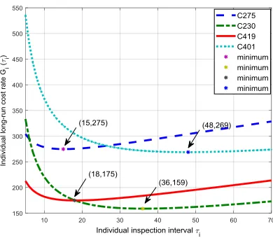
bearing (C401). Fig 7 shows how G_i (_i ) varies with _i of the four components.

Table 4 Optimal inspection policy for individual component

Component code

Optimal individual inspection interval

*

i

 (day)

Optimal individual long-run cost

rate *

( ) i i G  (€)

Sheathing C286 58 37

Sheathing C285 17 65

Tightness C275 15 275

Stub bearing C230 36 159

Tightness ring C460 19 36

Carrying bearing C419 18 175

Stub bearing C401 48 269

24

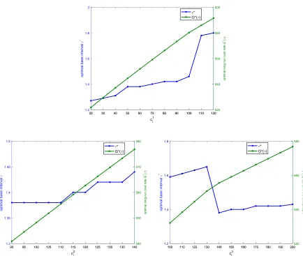
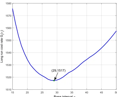
Fig 7 Plot of individual long-run cost rate

The common downtime cost is given as CI = €2500. According to Eq (7), the variation of

long-run cost rate G( ) with respect to the base interval  is plotted in Fig 8. From Fig 8, the

minimum long-run cost rate of €1517, obtained at the optimal base interval *29days. After

obtaining the optimal base interval *, we can determine the integral multiple k_i for each

component. The result is shown in Table 5. By comparing the results of Table 5 with the optimal

individual inspection interval, it is observed that the inspection period of stub bearing (C230) is

shifted in advance, the inspection period of sheathing (C286) remains unchanged, and the

inspection period of other components are postponed. Proposition 2 implies that the upper bound

of the base interval policy is at most sup









bound. In this section, the lower bound can be computed as LB = 1501. The long-run cost rate

25

Fig 8 Variation of ( )G with respect to base interval 

Table 5 Optimal inspection interval for base interval policy

Component code kiassociated with

optimal base interval

Optimal inspection

interval k_i (days)

Sheathing C286 2 58

Sheathing C285 1 29

Tightness C275 1 29

Stub bearing C230 1 29

Tightness ring C460 1 29

Carrying bearing C419 1 29

Stub bearing C401 2 58

Labyrinth support C780 2 58

Furthermore, in order to investigate how the components are grouped with various base

interval , we plot ki with respect to  in Fig 9. When  increases from 15 to 50 days, ki of the

components show a non-increasing trend. When  is no less than 41 days, k_i reduces to 1 for

1, 2,...,8

i , which implies that all the components are inspected at the same time. Note that we

only plot ki of four components (C286, C230, C401 and C780). ki of the other four components

26

Fig 9 Plot of k_i with respect to base interval 

Fig 10 shows how the optimal base interval * and the optimal long-run cost rate G*( ) vary

with the common downtime cost C_I. When C_I increases from €500 to €4500, *

( )

G  increase

monotonically from €1434 to €1582. In addition, the optimal base interval *

shows an

increasing trend with C_I , changing from 9 to 26 days. The result indicates that common

downtime cost has a significant influence on the optimal inspection policy. It is therefore

suggested that maintenance engineers or managers should take into account the common cost

(interactions among components) when making maintenance decisions for a multi-component

system.

27 6. Conclusions

This paper develops a maintenance policy for multi-component systems subject to hidden

failures. Failure of a component can only be detected at inspection and a failed component is

replaced once the failure is revealed. Different from previous works where an optimal inspection

interval is applied for the whole system, we obtain the optimal inspection interval for each

component. Concerned with the difficulty of the optimization problem, a heuristic method named

base interval approach is adopted to reduce the computational complexity. Upper bound of the

policy is analyzed, followed by two numerical examples. It is illustrated that that the base

interval policy can approximate the optimal policy within a small factor. The result of a

numerical example shows that our approach outperforms the individual inspection policy and the

common inspection policy.

The proposed maintenance strategy can be applied in various complex systems such as power

generators and processing facilities, especially for systems with a high common downtime cost.

One advantage of the proposed maintenance policy lies in its feasibility and applicability in

industry. Maintenance crews only need to inspect the components at fixed intervals and replace

the failed components, while no other tricky implementations are required.

Future research can be conducted by extending the present inspection-replacement policy into

a more general maintenance context. For example, consider a multi-component reparable system

where various maintenance actions such as minimal repair and imperfect maintenance are

allowed. In addition, if the components of the system follow a continuously degrading process

and the degrading state can be observed by inspection devices, one can integrate the concept of

base interval approach into condition-based maintenance and develop a more efficient

maintenance policy.

Acknowledgement

28 References

Ahmadi, A., & Kumar, U. (2011). Cost based risk analysis to identify inspection and restoration

intervals of hidden failures subject to aging. IEEE Transactions on Reliability, 60(1), 197-209.

Atkins, D., & Iyogun, P. (1987). A lower bound on a class of coordinated inventory/production

problems. Operations Research Letters, 6(2), 63-67.

Badia, F. G., Berrade, M. D., & Campos, C. A. (2001). Optimization of inspection intervals

based on cost. Journal of Applied Probability, 38(4), 872-881.

Camci, F. (2009). System maintenance scheduling with prognostics information using genetic

algorithm. IEEE Transactions on Reliability, 58(3), 539-552.

Cheng, Y., Chen, X., Ren, J., Xuan, X., & Li, X. (2013). Study on hidden failure of relay

protection in power system. IEEE Annual International Conference on Cyber Technology in

Automation Control and Intelligent Systems, Nanjing, China, 434-439.

Gao, Y., Feng, Y., Zhang, Z., & Tan, J. (2015). An optimal dynamic interval preventive

maintenance scheduling for series systems. Reliability Engineering & System Safety, 142, 19-30.

Gustavsson, E., Patriksson, M., Strömberg, A. B., Wojciechowski, A., & Önnheim, M. (2014).

Preventive maintenance scheduling of multi-component systems with interval costs. Computers

& industrial engineering, 76, 390-400.

He, K., Maillart, L. M., & Prokopyev, O. A. (2015). Scheduling Preventive Maintenance as a

Function of an Imperfect Inspection Interval. IEEE Transactions on Reliability, 64(3), 983-997.

Hopp, W. J., & Kuo, Y. L. (1998). Heuristics for multi-component joint replacement:

Applications to aircraft engine maintenance. Naval Research Logistics, 45(5), 435-458.

Huynh, K. T., Barros, A., & Berenguer, C. (2015). Multi-Level Decision-Making for The

Predictive Maintenance of-Out-of-: F Deteriorating Systems. IEEE Transactions on Reliability,

29

Jackson, P., Maxwell, W., & Muckstadt, J. (1985). The joint replenishment problem with a

powers-of-two restriction. IIE Transactions, 17(1), 25-32.

Laggoune, R., Chateauneuf, A., & Aissani, D. (2009). Opportunistic policy for optimal

preventive maintenance of a multi-component system in continuous operating units. Computers

& Chemical Engineering, 33(9), 1499-1510.

Lam, J. Y. J., & Banjevic, D. (2015). A myopic policy for optimal inspection scheduling for

condition based maintenance. Reliability Engineering & System Safety, 144, 1-11.

Levi, R., Magnanti, T., Muckstadt, J., Segev, D., & Zarybnisky, E. (2014). Maintenance

scheduling for modular systems: Modeling and algorithms. Naval Research Logistics (NRL),

61(6), 472-488.

Liu, B., Wu, J., & Xie, M. (2015). Cost analysis for multi-component system with failure

interaction under renewing free-replacement warranty. European Journal of Operational

Research, 243(3), 874-882.

Liu, B., Wu, S., Xie, M., & Kuo, W. (2017). A condition-based maintenance policy for

degrading systems with age-and state-dependent operating cost. European Journal of

Operational Research, 263(3), 879-887.

Liu, B., Xie, M., Xu, Z., & Kuo, W. (2016). An imperfect maintenance policy for

mission-oriented systems subject to degradation and external shocks. Computers & Industrial

Engineering, 102, 21-32.

Liu, B., Xu, Z., Xie, M., & Kuo, W. (2014). A value-based preventive maintenance policy for

multi-component system with continuously degrading components. Reliability Engineering &

System Safety, 132, 83-89.

Nicolai, R. P., & Dekker, R. (2008). Optimal maintenance of multi-component systems: a

review (pp. 263-286). Springer London.

Pandey, M., Zuo, M. J., & Moghaddass, R. (2015). Selective maintenance scheduling over a

finite planning horizon. Proceedings of the Institution of Mechanical Engineers, Part O: Journal

30

Peng, H., Feng, Q., & Coit, D. W. (2010). Reliability and maintenance modeling for systems

subject to multiple dependent competing failure processes. IIE Transactions, 43(1), 12-22.

Phan, D. T., & Zhu, Y. (2015). Multi-stage optimization for periodic inspection planning of

geo-distributed infrastructure systems. European Journal of Operational Research, 245(3), 797-804.

Taghipour, S., & Banjevic, D. (2011). Periodic inspection optimization models for a repairable

system subject to hidden failures. IEEE Transactions on Reliability, 60(1), 275-285.

Tian, Z., & Liao, H. (2011). Condition based maintenance optimization for multi-component

systems using proportional hazards model. Reliability Engineering & System Safety, 96(5),

581-589.

Vu, H. C., Do, P., Barros, A., & Berenguer, C. (2014). Maintenance grouping strategy for

multi-component systems with dynamic contexts. Reliability Engineering & System Safety, 132,

233-249.

Wang, H. (2002). A survey of maintenance policies of deteriorating systems. European Journal

of Operational Research, 139(3), 469-489.

Wang, H. K., Huang, H. Z., Li, Y. F., & Yang, Y. J. (2016). Condition-Based Maintenance With

Scheduling Threshold and Maintenance Threshold. IEEE Transactions on Reliability, 65(2),

513-524.

Wang, Y., & Pham, H. (2011). A multi-objective optimization of imperfect preventive

maintenance policy for dependent competing risk systems with hidden failure. IEEE

Transactions on Reliability, 60(4), 770-781.

Xiao, L., Song, S., Chen, X., & Coit, D. W. (2016). Joint optimization of production scheduling

and machine group preventive maintenance. Reliability Engineering & System Safety, 146, 68-78.

Xiao, X., & Ye, Z. (2016). Optimal design for destructive degradation tests with random initial

31

Yang, F., Meliopoulos, A. S., Cokkinides, G. J., & Binh Dam, Q. (2006). Effects of protection

system hidden failures on bulk power system reliability. Proceedings of the 38th Annual North

American Power Symposium, 517-523.

Ye, Z., Revie, M., & Walls, L. (2014). A Load Sharing System Reliability Model With Managed

Component Degradation. IEEE Transactions on Reliability, 63(3), 721-730.

Ye, Z. S., & Xie, M. (2015). Stochastic modelling and analysis of degradation for highly reliable

products. Applied Stochastic Models in Business and Industry, 31(1), 16-32.

Zhang, M., Gaudoin, O., & Xie, M. (2015). Degradation-based maintenance decision using

stochastic filtering for systems under imperfect maintenance. European Journal of Operational

Research, 245(2), 531-541.

Zhu, W., Fouladirad, M., & Berenguer, C. (2016). A level maintenance policy for a

multi-component and multifailure mode system with two independent failure modes. Reliability

Engineering & System Safety, 153, 50-63.

Appendix

1. Proof of Proposition 1.

( )

i i

G  can be rewritten as

( )

( ) i i

i i d i U

G  c 



  ,

where

0 0

( )_{i d}i _{i r}i i_{I i}( _i) / _i( _i)

j j

U  c  c c R j R j

 

 

 

 _   _







After some simplifications, U( )_i is expressed as U( )_i  c_Ii







Obviously,

0 i( i)

j R j

 



0

lim ( ) 1

i

i i j R j

 

 





thatcdii cri cIi, then we have ( ) , (0, )

i

i i d i

G  c    . Moreover, lim ₀ ( ) 1

i

i i j R j

 

 





that lim ( )

i

i i i d

G c

   , leading to the conclusion that

*