Optimal Capital Allocation Principles

City, University of London Institutional Repository

Citation:

Dhaene, J., Tsanakas, A., Valdez, E. A. and Vanduffel, S. (2012). Optimal Capital Allocation Principles. Journal of Risk and Insurance, 79(1), pp. 1-28. doi: 10.1111/j.1539-6975.2011.01408.x

This is the accepted version of the paper.

This version of the publication may differ from the final published

version.

Permanent repository link:

http://openaccess.city.ac.uk/5982/

Link to published version:

http://dx.doi.org/10.1111/j.1539-6975.2011.01408.x

Copyright and reuse: City Research Online aims to make research

outputs of City, University of London available to a wider audience.

Copyright and Moral Rights remain with the author(s) and/or copyright

holders. URLs from City Research Online may be freely distributed and

linked to.

City Research Online: http://openaccess.city.ac.uk/ [email protected]

Electronic copy available at: http://ssrn.com/abstract=1332264Electronic copy available at: http://ssrn.com/abstract=1332264

Jan Dhaene†‡ _{Andreas Tsanakas}§ _{Emiliano A. Valdez}¶ _{Steven Vanduffel} k

April 20, 2010

Abstract

This paper develops a unifying framework for allocating the aggregate capital of a financial firm to its business units. The approach relies on an optimisation argument, requiring that the weighted sum of measures for the deviations of the business unit’s losses from their re-spective allocated capitals be minimised. The approach is fair insofar as it requires capital to be close to the risk that necessitates holding it. The approach is additionally very flexible in the sense that different forms of the objective function can reflect alternative definitions of corporate risk tolerance. Owing to this flexibility, the general framework reproduces several capital allocation methods that appear in the literature and allows for alternative interpreta-tions and possible extensions.

Keywords: Capital allocation; risk measure; comonotonicity; Euler allocation; default op-tion; optimisation.

1

Introduction

The level of the capital held by a bank or an insurance company is a key issue for its stakeholders. The regulator, primarily sharing the interests of depositors and policyholders, establishes rules to determine the required capital to be held by the company. The level of this capital is determined such that the company will be able to meet its financial obligations with a high probability as they fall due, even in adverse situations. Rating agencies rely on the level of available capital to assess the financial strength of a company. Shareholders and investors alike are concerned with the risk of their capital investment and the return that it will generate.

The determination of a sufficient amount of capital to hold is only part of a larger risk man-agement and solvency policy. The practice of Enterprise Risk Manman-agement (ERM) enhances identifying, measuring, pricing, and controlling risks. An important component of an ERM framework is the exercise ofcapital allocation, a term referring to the subdivision of the aggre-gate capital held by the firm across its various constituents, e.g. business lines, types of exposure, territories or even individual products in a portfolio of insurance policies.

Most financial firms write several lines of business and may want their total capital allocated across these lines for a number of reasons. First, there is a need to redistribute the total (fric-tional or opportunity) cost associated with holding capital across various business lines so that this cost is equitably transferred back to the depositors or policyholders in the form of charges.

∗_{An early draft of this paper was presented at the 9th International Congress on Insurance: Mathematics and}

Economics (IME2005) in Laval, Quebec, Canada.

†_{Corresponding author: [email protected] (phone: +32 16 326750)} ‡_{Faculty of Business and Economics, Katholieke Universiteit, Leuven, Belgium.} §_{Cass Business School, City University, London, United Kingdom.}

¶

Department of Mathematics, University of Connecticut, Storrs, Connecticut, USA.

k_{Department of Economics and Political Science, Vrije Universiteit Brussel (VUB), Brussel, Belgium.}

Electronic copy available at: http://ssrn.com/abstract=1332264Electronic copy available at: http://ssrn.com/abstract=1332264

Secondly, the allocation of expenses across lines of business is a necessary activity for financial reporting purposes. Thirdly, capital allocation provides for a useful device of assessing and com-paring the performance of the different lines of business by determining the return on allocated capital for each line. Comparing these returns allows one to distinguish the most profitable busi-ness lines and hence may assist in remunerating the busibusi-ness line managers. Finally, allocating capital may help to identify areas of risk consumption within a given organisation and support the decision making concerning business expansions, reductions or even eliminations.

There is a countless number of ways to allocate the aggregate capital of a company to its different business units. Mutual dependencies that may exist between the performances of the various business units make capital allocation a non-trivial exercise. Accordingly, there is an extensive amount of literature on this subject with a wide number of proposed capital allocation algorithms. Cummins (2000) provides an overview of several methods suggested for capital al-location in the insurance industry and relates capital alal-location to management decision making tools such as RAROC (risk-adjusted return on capital) and EVA (economic value added). Myers and Read Jr. (2001) consider capital allocation principles based on the marginal contribution of each business unit to the company’s default option. LeMaire (1984) and Denault (2001) discuss capital allocations based on game theoretic considerations, where a risk measure is used as a cost functional. In the case of coherent risk measures (see Artzner et al. (1999)), such capi-tal allocations reduce to subdivisions according to marginal costs. Overbeck (2000) considers marginal contributions to the expected shortfall risk measure in a credit risk context. In closely related works, marginal (‘Euler’) capital allocations are proposed within a portfolio optimisation context by Tasche (2004) and an axiomatic allocation system is proposed by Kalkbrener (2005). A commentary on the various approaches to allocating capital has appeared in Venter (2004). A recent work by Kim and Hardy (2008) proposed a method based on a solvency exchange option and which explicitly accounts for the notion of limited liability.

Panjer (2001) considers the particular case of multivariate normally distributed risks and provides an explicit expression of marginal cost based allocations, when the risk measure used is Tail Value-at-Risk (TVaR). Landsman and Valdez (2003) extends these explicit capital alloca-tion formulas to the case where risks belong to the class of multivariate elliptical distribualloca-tions, for which the class of multivariate normal is a special case. Dhaene et al. (2008) re-derive the results of Landsman and Valdez (2003) in a more straightforward manner and apply these to sums that involve normal as well as lognormal risks. In Valdez and Chernih (2003), expressions for covariance-based allocations are derived for multivariate elliptical risks. Tsanakas (2004) studies allocations where the relevant risk measure belongs to the class of distortion risk mea-sures, while Tsanakas (2008) extends these allocation principles to the more general class of convex risk measures including the exponential risk measures. By considering the link between solvency and a fair rate of return, Sherris (2006) developed allocation principles consistent with the economic value of a financial institution’s balance sheet. Furman and Zitikis (2008b) in-troduce the class of weighted risk capital allocations “which stems from the weighted premium calculation principle”.

The multitude of allocation methods proposed in the literature can be bewildering, with the justifications of allocation approaches varying between e.g. economic (Tasche, 2004), game-theoretic (Denault, 2001), and axiomatic (Kalkbrener, 2005) criteria, while some authors doubt the purpose itself of allocating capital (Gr¨undl and Schmeiser, 2007; Phillips et al., 1998; Venter, 2004).

• The idea of capital being ‘close’ to the risk it is being allocated to is intuitive because allocated capital should be a reflection of the associated risk. Moreover, such closeness models a notion of fairness within an organisation: risky portfolios are penalised, less risky ones are rewarded.

• The objective function of our optimisation approach relies crucially on the function used to weigh, that is, define the significance, of different scenarios (states of the world). Conse-quently, capital is allocated such that it matches closely the risk under particular scenarios considered adverse by management. These may be scenarios affecting the whole portfolio or isolated business units, extreme or less extreme, depending solely on the company’s aggregate risk or on broader market conditions. Thus the proposed approach allows the flexibility of aligning capital allocation with management’s different notions of risk toler-ance.

It is then shown that many capital allocation approaches appearing in the literature can be seen as special cases of our more general framework. Thus different allocation approaches, studied through a common framework, are made comparable and are offered an alternative interpretation. A quadratic deviation criterion gives rise to allocations that generally have the form of expectations. Allocations based on well-known risk measures such as the Conditional Tail Expectation (CTE) (e.g. as in Overbeck (2000)) as well as allocations taking into account the insurer’s default option (e.g. as in Sherris (2006)) are derived in this setting. An absolute deviation criterion gives rise to quantile-based allocations, whereby diversification is reflected by lowering the confidence level of VaR measures applied at sub-portfolio level. In both cases, the allocations may or may not reflect the dependence structure of the portfolio, via dependence between the individual and the aggregate risks.

The purpose of our approach is not to choose a “best possible” capital allocation method, but instead, by considering very different capital allocation formulas as part of the same framework in order to make these more comparable and mutually illuminating.

We note that mathematical results related to the material in this paper have been presented by Zaks et al. (2006). These authors work in a premium allocation context, restricting them-selves to quadratic deviation criteria and do not use the device of weighting different scenarios; the range of allocation approaches derived in that paper is therefore narrower in scope. It is to be noted that the idea of deriving capital allocation via optimisation arguments was also discussed by Dhaene et al. (2003) and Laeven and Goovaerts (2004). However, Dhaene et al. (2003) is within the scope of our general framework while Laeven and Goovaerts (2004) generalizes Dhaene et al. (2003) but in a different direction than ours.

The structure of the rest of the paper is as follows. In Section 2, risk measures and the capital allocation problem are discussed and an overview of some popular allocation methods is given. In Section 3, which forms the main contribution of the paper, a unifying optimal capital allocation approach is presented. From this general approach, a multitude of special cases is derived. Finally, brief conclusions are given in Section 4.

2

Capital allocation

2.1 Risk Measures

A risk measure is a mappingρfrom a setΓof real-valued random variables defined on a proba-bility space(Ω,F,P)to the real lineR:

The random variable X refers to the loss associated with conducting a business. In actuar-ial science, risk measures have traditionally been used for determining insurance premiums (Goovaerts et al. (1984)). More recently, however, they have been applied in a risk manage-ment context, withρ[X]representing the amount of capital to be set aside in order to make the lossX an acceptable risk; see Artzner et al. (1999).

Some well known properties that risk measures may or may not satisfy are law invariance, monotonicity, positive homogeneity, translation invariance (or equivariance) and subadditivity. They are formally defined as:

• Law invariance: For any X1, X2 ∈ Γ withP[X1 ≤ x] = P[X2 ≤ x]for allx ∈ R,ρ[X1] =

ρ[X2].

• Monotonicity: For anyX1, X2 ∈Γ,X1 ≤X2impliesρ[X1]≤ρ[X2].

• Positive homogeneity: For anyX ∈Γanda >0,ρ[aX] =aρ[X]. • Translation invariance: For anyX∈Γandb∈_R,ρ[X+b] =ρ[X] +b. • Subadditivity: For anyX1, X2 ∈Γ,ρ[X1+X2]≤ρ[X1] +ρ[X2].

Artzner et al. (1999) call any risk measure that satisfies the last four properties a coherent risk measure. F¨ollmer and Schied (2002) provide weaker sets of properties and discuss the desirability or otherwise of the properties of coherent risk measures.

2.2 The allocation problem

Consider a portfolio of nindividual losses X1, X2, ..., Xnmaterialising at a fixed future dateT.

Assume that(X1, X2, ..., Xn)is a random vector on the probability space(Ω,F,P). Throughout

the paper, we will always assume that any lossXi has a finite mean. The distribution function

P[Xi ≤x]ofXiwill be denoted byFXi(x).

The aggregate loss is defined by the sum

S =

n

X

i=1

Xi, (2)

where this aggregate lossS can be interpreted as:

• the total loss of a corporate, e.g. an insurance company, with the individual losses corre-sponding to the losses of the respective business units;

• the loss from an insurance portfolio, with the individual losses being those arising from the different policies; or

• the loss suffered by a financial conglomerate, while the different individual losses corre-spond to the losses suffered by its subsidiaries.

It is the first of these interpretations we will use throughout this article. Hence S is the aggregate loss faced by an insurance company and Xi the loss of business unit i. We assume

across its various business units, that is, to determine non-negative real numbers K1, . . . , Kn

satisfying the full allocation requirement:

n

X

i=1

Ki=K. (3)

This allocation is in some sense a notional exercise; it does not mean that capital is physically shifted across the various units, as the company’s assets and liabilities continue to be pooled. The allocation exercise could be made in order to rank the business units according to levels of profitability. This task can be performed, for example, by determining the returns on the allocated capital for the respective business units.

Given that a capital allocation can be carried out in a countless number of ways, additional criteria must be set up in order to determine the most suitable. A reasonable start is to require the allocated capital amounts Ki to be ‘close’ to their corresponding lossesXi in some

appro-priately defined sense. This underlies the approach proposed in the present paper. Prior to introducing the idea of ‘closeness’ between individual loss and allocated capital, we revisit some well-known capital allocation methods.

2.3 Some known allocation formulas

For a given probability levelp∈(0,1), we denote the Value-at-Risk (VaR) or quantile of the loss random variableXbyF_X−1(p). As usual, it is defined by

F_X−1(p) = inf{x∈_R|FX(x)≥p}, p∈[0,1]. (4)

with inf{∅} = +∞ by convention. Below we will also need so-called α–mixed inverse distri-bution functions; see Dhaene et al. (2002). Therefore, we first define the inverse distridistri-bution functionF_X−1+(p)of the random variableXby

F_X−1+(p) = sup{x∈_R|FX(x)≤p}, p∈[0,1], (5)

withsup{∅}= −∞. Theα–mixed inverse distribution functionF_X−1(α) ofX is then defined as follows:

F_X−1(α)(p) =αF_X−1(p) + (1−α)F_X−1+(p), p∈(0,1)α∈[0,1]. (6) From this definition, one immediately finds that for any random variable X and for all x with 0< FX(x)<1, there exists anαx ∈[0,1]such thatF_X−1(αx)(FX(x)) =x.

2.3.1 The haircut allocation principle

It is a common industry practice, driven by banking and insurance regulations, to measure stand-alone losses by a VaR for a given probability levelp. In line with such practice, a straightforward allocation method consists of allocating the capitalKi=γF_X−_i1(p),i= 1, . . . , n, to business unit

i, where the factor γ is chosen such that the full allocation requirement (3) is satisfied. This gives rise to thehaircut allocation principle:

Ki=

K

Pn

j=1F

−1

Xj(p)

F_X−1

i(p), i= 1, . . . , n. (7)

For an exogenously given value ofK, this principle leads to an allocation that is not influ-enced by the dependence structure between the lossesXiof the different business units. In this

It is well-known that the quantile risk measure is not always subadditive. Consequently, using thep-quantile as stand-alone risk measure will not necessarily imply that the subportfolios will benefit from a pooling effect. This means that it may happen that the allocated capitalsKi

exceed the respective stand-alone capitalsF_X−1

i(p).

2.3.2 The quantile allocation principle

The haircut allocation rule (7) allocates to each business unitia proportion γ of itsp-quantile, with γ chosen such that the full allocation condition is fulfilled. This means that a constant proportional reduction (or increase) is applied on each of the quantiles F_X−1

i(p). Instead of

applying a proportional cut on the monetary amountsF_X−1

i(p), one could adopt the probability

levelpequally among all business units and determine anα–mixed inverse withα∈[0,1], such that the full allocation requirement is again satisfied. This approach gives rise to the quantile allocation principlewith allocated capital amountsKi given by

Ki=F

−1(α)

Xi (βp), withαandβ such that

n

X

i=1

Ki =K. (8)

Similar to the haircut allocation principle, for a given aggregate capitalK, the allocated capitals

Ki are not influenced by the dependence structure between the different lossesXi,i= 1, . . . , n.

The quantile allocation rule is in compliance with the principle of using equal quantiles to measure the risk associated with the different business units. If it is considered ‘consistent’ to measure each stand-alone lossXiby the corresponding quantileFX−i1(p), then it makes sense to

measure each ‘pooled’ loss byF_X−1(α)

i (βp)whereαandβare chosen such that the full allocation

requirement is satisfied. This means that all losses Xi continue to be evaluated at the same

probability level ‘β×p’ and the benefits from pooling are in some sense ‘subdivided neutrally’ across the different business units.

The haircut allocation principle (7) will in general not lead to a quantile-based allocation with the same probability level for all business units. Companies and regulators when debating that all risks should be evaluated using the same p-quantile measure may prefer the quantile allocation principle rather than the haircut principle.

The appropriate levels ofαandβ are to be determined as the solutions to

K =

n

X

i=1

F_X−1(α)

i (βp), (9)

In order to solve this problem, we need to introduce the concept of acomonotonic sumScdefined by

Sc=

n

X

i=1

F_X−1

i(U), (10)

whereU is a uniform random variable on(0,1). It then holds that

K =F_S−c1(α)(βp), (11)

which leads us to

βp=FSc(K). (12)

Furthermore, we have that

Further additional details can be found in Dhaene et al. (2002). The quantile allocation rule in (8) can then be re-expressed as

Ki=F

−1(α)

Xi (FSc(K)), i= 1, . . . , n, (14)

withαdetermined from (13).

In the special case that all distribution functionsFXi are strictly increasing and continuous,

this rule reduces to

Ki=F_X−_i1(FSc(K)), i= 1, . . . , n. (15)

This allocation principle was proposed in Dhaene et al. (2003), where it was derived as the solution of an appropriate optimisation problem; See also Section 3.3. Notice that for strictly increasing and continuous distribution functions FXi, the quantile allocation principle can be

considered as a special case of the haircut allocation principle (7) by choosingp=FSc(K).

2.3.3 The covariance allocation principle

Thecovariance allocation principleproposed by e.g. Overbeck (2000) is given by

Ki =

K

Var[S]Cov[Xi, S], i= 1, . . . , n, (16) where Cov[Xi, S] is the covariance between the individual loss Xi and the aggregate loss S

and Var[S]is the variance of the aggregate lossS. Because clearly the sum of these individual covariances is equal to the variance of the aggregate loss, the full allocation requirement is automatically satisfied in this case.

The covariance allocation rule, unlike the haircut and the quantile allocation principles, ex-plicitly takes into account the dependence structure of the random losses(X1, X2, ..., Xn).

Busi-ness units with a loss that is more correlated with the aggregate portfolio loss S are penalised by requiring them to hold a larger amount of capital than those which are less correlated.

2.3.4 The CTE allocation principle

For a given probability levelp ∈(0,1), the Conditional Tail Expectation (CTE) of the aggregate lossS is defined as

CTEp[S] =ES |S > FS−1(p)

. (17)

At a fixed level p, it gives the average of the top (1−p)% losses. In general, the CTE as a risk measure does not necessarily satisfy the subadditivity property. However, it is known to be a coherent risk measure in case we restrict to random variables with continuous distribution function. See e.g. Acerbi and Tasche (2002) and Remark 4.2.3. in Dhaene et al. (2006).

TheCTE allocation principle, for some fixed probability levelp∈(0,1), has the form

Ki =

K

CTEp[S]E

Xi

S > F_S−1(p)

, i= 1, . . . , n (18)

In the particular case thatK =CTEp[S], formula (18) essentially reduces to the “contributions

to expected shortfall” allocation suggested by Overbeck (2000) and, as a special case, by Denault (2001). In fact, the CTE allocation principle is a special case of marginal or Euler allocations discussed in detail by Tasche (2004).

The CTE allocation rule explicitly takes into account the dependence structure of the random losses(X1, X2, ..., Xn). Imterpreting the event ‘S > F_S−1(p)’ as ‘the aggregate portfolio loss Sis

2.3.5 Proportional allocations

The capital allocation methods we have discussed so far can also be viewed as special cases of a more general class. Each member of this class is obtained by first choosing a risk measureρ

and then attributing the capital Ki = αρ[Xi]to each business unit i, i = 1, . . . , n. The factor

α is chosen such that the full allocation requirement (3) is satisfied. This gives rise to the proportional allocation principle:

Ki=

K

Pn

j=1ρ[Xj]

ρ[Xi], i= 1, . . . , n. (19)

The allocation principles discussed in the previous subsections follow from (19) by choosing the appropriate risk measureρ:

Haircut allocation: ρ[Xi] =FX−i1(p), (20)

Quantile allocation: ρ[Xi] =F_X−_i1(FSc(K)) withαfrom (13), (21)

Covariance allocation: ρ[Xi] =Cov[Xi, S], and (22)

CTE allocation: ρ[Xi] =EXi

S > F_S−1(p)

. (23)

We note that in the last two allocations, the risk measure ρ(X) does not depend only on the distribution ofX, that is,ρis not law invariant. Ifρis law invariant (first two allocations), the proportional allocation derived fromρ is not influenced by the dependence structure between the lossesXiof the different business units.

Let us assume that stand-alone losses are measured by a risk measure ρ. This means that

K =ρ[S]and also that the risk of business uniti, considered as a stand-alone unit, is measured by ρ[Xi]. From (19) one finds that in case of a proportional allocation, each business unit

benefits from a pooling effect in the sense thatKi≤ρ[Xi]if and only if

K =ρ[S]≤

n

X

j=1

ρ[Xj]. (24)

This condition is fulfilled for subadditive risk measures ρ. As we have observed before, the haircut allocation method, which chooses a VaR as a stand-alone risk measure, may lead to a positive or a negative pooling effect. On the other hand, choosing Tail Value-at-Risk (TVaR) as stand-alone risk measure such as in the CTE allocation method, will lead toKi ≤ρ[Xi].

In Section 3, we develop a unifying optimal capital allocation approach and show that the quantile allocation (21), the covariance allocation (22) and the CTE allocation (23) fall as spe-cial cases of this approach. In contrast, the haircut allocation (20) does not seem to be recon-cilable with our general framework. Note however that for strictly increasing and continuous distribution functionsFXi, the quantile allocation principle can be considered as a special case

of the haircut allocation principle by choosingp=FSc(K).

2.3.6 Location-scale families of distributions

This section investigates the relationship that exists between the different allocation rules pre-sented above, in case the losses Xi belong to the same location-scale family of distributions.

Herewith, we assume that there exists a random variable Z with a zero mean and constants

ai >0andbi such that

Xi d

=aiZ+bi, i= 1, . . . , n, (25)

where=d stands for ‘equality in distribution’. For simplicity, we further assume thatFZ is strictly

Let us first consider the general proportional allocation principle (19) whereρis assumed to be law invariant, translation invariant and positive homogeneous. In this case, all ρ[Xi]can be

expressed as

ρ[Xi] =F_X−_i1(p) =ai+zpbi, i= 1, . . . , n, (26)

where zp is thep-th quantile ofZ for some fixed probability levelp ∈ (0,1); see e.g. Dhaene

et al. (2009). This means that under the stated conditions, the proportional allocation principle (19) reduces to the haircut allocation principle (7).

Next we consider the CTE allocation principle (18) withK =CTEp[S]and where the vector

of business losses (X1, X2, ..., Xn) is multivariate elliptically distributed with E[Xi] = 0, i =

1, . . . , n. The assumption that allXi have a zero mean may be relevant for practical situations

where a provision equal to the expected value of the aggregate loss is set aside, and in addi-tion capital is used as a buffer to protect against the ‘uncertainty of the aggregate loss around its mean’. In this case, each Xi has to be interpreted as the loss of business unit i minus its

expectation.

From Landsman and Valdez (2003), we find that in this case the allocated capitalsKi are

given by

Ki=EXi

S > F

−1

S (p)

= CTEp[S]

Var[S] Cov[Xi, S], i= 1, . . . , n. (27) Hence, we can conclude that when (X1, X2, ..., Xn) is multivariate elliptically distributed with

zero means and in addition K =CTEp[S], the CTE allocation principle (18) coincides with the

covariance allocation principle (16).

2.3.7 Allocation and the default option

A somewhat different class of approaches, based on the arguments of Myers and Read Jr. (2001), produces a capital allocation procedure by considering the value of the insurer’s default option. Since the shareholders of the company have limited liability, in the event of default, i.e. when

S > K, they are not, in principle, obligated to pay the excess loss S −K. Therefore, the protection that the collective of policyholders purchases ismin(S, K), which can be written as

S−(S−K)+. (28) The quantity(S−K)+is called thepolicyholder deficitor alternatively theinsurer’s default option. Myers and Read Jr. (2001) assume that markets are complete and that a proportional in-crease in the exposure to a particular line of business produces a proportional inin-crease in its allocated capital. They subsequently allocate the value of the default option via the marginal contributions of each line of business to that value.

It can be shown that the Myers-Read allocation is given by the general formula (which does not appear in their paper in this form),

E[(S−K)+] =

n

X

j=1

E[(Xj−Kj)I(S > K)], (29)

where I(A) is the indicator function of event A and expectations may be taken under a risk

neutral measure.

It is worth noting that (29) is not a capital allocation formula in itself, as theK1. . . , Knare

3

Optimal capital allocations

3.1 General setting

The allocation of the exogenously given aggregate capitalK tonpartsK1, . . . , Kn,

correspond-ing to the different subportfolios or business units, can be carried out in an infinite number of ways, some of which were illustrated in the previous section. At first glance, there seems to be a lack of a clear motivation for preferring to choose one method over another, although it appears obvious that different capital allocations must in some sense correspond to different questions that can be asked within the context of risk management. Hereafter we systematise capital allo-cation methods by viewing them as solutions to a particular decision problem. For that we need to formulate a decision criterion, such as:

Capital should be allocated such that for each business unit the allocated capital and the loss are sufficiently close to each other.

In order to cast this statement in a more formal setting, consider the aggregate portfolio loss

S = X1 +· · ·+Xn with aggregate capital K. Once the aggregate capital is allocated, the

difference between aggregate loss and aggregate capital can be expressed as

S−K =

n

X

j=1

(Xj−Kj), (30)

where the quantity (Xj−Kj)expresses the loss minus the allocated capital for subportfolioj.

Important to notice is that in this setting, the subportfolios are cross-subsidising each other, in the sense that the occurence of the event ‘Xk > Kk’ does not necessarily lead to ‘ruin’; such

unfavorable performance of subportfoliokmay be compensated by a favorable outcome for one or more values(Xl−Kl)of the other subportfolios.

We propose to determine the appropriate allocation by the following optimisation problem:

Optimal capital allocation problem: Given the aggregate capitalK >0, determine the allocated capitalsKi, i= 1, . . . , n,from the following optimisation problem:

min

K1,...,Kn

n

X

j=1

vjE

ζj D

Xj−Kj

vj

, such that

n

X

j=1

Kj =K, (31)

where thevjare non-negative real numbers such thatPn_j=1vj = 1, theζj are non-negative random

variables such thatE[ζj] = 1and D is a non-negative function.

Before solving the general optimal capital allocation problem (31), we first elaborate on its various elements.

vj : The non-negative real number vj is a measure of exposure or business volume of the j

-th unit, such as revenue, insurance premium, etc. These scalar quantities are chosen such that they sum to 1. Their inclusion in the expression DXj−Kj

vj

normalises the deviations of loss from allocated capital across business units to make them relatively more comparable. At the same time, thevj’s are used as weights attached to the different values

of E

h

ζj D

_X

j−Kj

vj i

DXj−Kj

vj

: For simplicity, we first assume that vj = 1 and also that ζj ≡ 1. The terms

D(Xj−Kj)quantify the deviations of the outcomes of the lossesXj from their allocated

capitalKj. Minimising the sum of the expectations of these quantities essentially reflects

the requirement that the allocated capitals should be ‘as close as possible’ to the losses they are allocated to. Examples of distance measures are “squared or quadratic deviations” and “absolute deviations”.

ζj : The deviations of the losses Xj from their respective allocated capital levels Kj are

mea-sured by the terms E[ζj D(Xj−Kj)]. These expectations involve non-negative random

variables ζj with E[ζj] = 1 that are used as weight factors to the different possible

out-comes ofD(Xj −Kj).

One possible choice for the ζj could be ζj = h(Xj) for some negative and

non-decreasing function h. In this case, the heaviest weights are attached to deviations that correspond to states-of-the-world leading to the largest outcomes ofXj. We will call

allo-cations based on such a choice for theζj business unit driven allocations.

Another choice is to let ζj =h(S) for some non-negative and non-decreasing functionh,

such that the outcomes of the deviations are weighted with respect to the aggregate port-folio performance. In this case, heavier weights are attached to deviations that correspond to states-of-the-world leading to larger outcomes ofS. Allocations based on such a choice for the random variablesζj will be calledaggregate portfolio driven allocations.

A yet different approach is to letζj =ζM for allj, whereζM can be interpreted as the loss

on a reference (or market) portfolio. In this case, the weighting is market driven and the corresponding allocation is said to be amarket driven allocation.

In summary, we propose in (31) to fully allocate the aggregate capitalK to the different business units such that the exposure-weighted sum of the expectations of the weighted and normalised deviations of the lossesXj from their respective allocated capitalsKj, is minimised.

3.2 The quadratic optimisation criterion

3.2.1 General solution of the quadratic allocation problem

In this subsection we discuss optimal allocation under a quadratic criterion, that is, by letting

D(x) =x2. (32) In this case, the optimal allocation problem (31) reduces to

min

K1,...,Kn

n

X

j=1

E

"

ζj

(Xj−Kj)2

vj

#

, such that

n

X

j=1

Kj =K. (33)

The solution to this minimisation problem is given in the following theorem.

Theorem 1 The optimal allocation problem (33) has the following unique solution:

Ki =E[ζiXi] +vi



K−

n

X

j=1

E[ζjXj]



, i= 1, . . . , n. (34)

Taking into account the relations

E

h

ζj(Xj−Kj)2

i

= (E[ζjXj]−Kj)2+EζjXj2

−(E[ζjXj])2, j= 1, . . . , n,

we have that the solution of the minimisation problem (33) is identical to the solution of the following minimisation problem:

min

K1,...,Kn

n

X

j=1

(E[ζjXj]−Kj)2

vj

, such that

n

X

j=1

Kj =K. (35)

Clearly, eliminating the term Pn

j=1

E

h

ζjXj2

i

−(E[ζjXj])2

does not change the optimal allo-cation.

By introducing the notation

xj =

Kj−E[ζjXj]

√

vj

j= 1, . . . , n, (36)

we can transform (35) into

min

x1,...,xn

n

X

j=1

x2_j, such that

n

X

j=1

√

vjxj =



K−

n

X

j=1

E[ζjXj]



. (37)

Let us now interpret the set







(x1, x2, . . . , xn)∈Rn

n X j=1 √

vjxj =



K−

n

X

j=1

E[ζjXj]



 





as a hyperplane inRn. The solution of (37) can then be interpreted as the point(x1, x2, . . . , xn)

on the hyperplanePn

j=1

√

vjxj =

K−Pn

j=1E[ζjXj]

that is closest to the origin(0,0, . . . ,0). Hence,

xi =

√

vi



K−

n

X

j=1

E[ζjXj]



, i= 1, . . . , n.

Translating this result in terms of theKivia (36) immediately leads to (34).

The capitalKi given by (34) equals the weighted expected loss ofXi, in addition to a term

proportional to the volume of the unit. This second term is a redistribution of the difference between the amount of aggregate capital K held and Pn

j=1E[ζjX]. This redistribution is

as-signed using weightsvi based on the ‘volume’ or on some other measure of the ‘riskiness’ of the

corresponding business units.

In the particular case that the volume weights are given by

vi= E

[ζiXi]

Pn

j=1E[ζjXj]

, (38)

it immediately follows that (34) reduces to

Ki =

K

Pn

j=1E[ζjXj]E

This allocation rule can be seen as a special case of the proportional allocation rule (19), by choosing

ρ[Xi] =E[ζiXi], i= 1, . . . , n. (40)

Notice that (39) can be rearranged as

Ki−E[ζiXi]

E[ζiXi]

= K−

Pn

j=1E[ζjXj]

Pn

j=1E[ζjXj]

, i= 1, . . . , n. (41)

In the special case that the aggregate capitalKis given byK =Pn

j=1E[ζjXj], the allocation

rule (34) reduces to

Ki =E[ζiXi], i= 1, . . . , n. (42)

This class of allocations is investigated in Furman and Zitikis (2008b) who call the members of this classweighted risk capital allocations.

3.2.2 Business unit driven allocations

In this subsection we consider the case where the weighting random variablesζiin the quadratic

allocation problem (33) are given by

ζi =hi(Xi), (43)

with hi being a non-negative and non-decreasing function such that E[hi(Xi)] = 1, for i =

1, . . . , n. Hence, for each business uniti, the states-of-the-world to which we want to assign the heaviest weights are those under which the business unit performs the worst. As earlier pointed out, we call allocations based on (43)business unit driven allocations. In this case, the allocation rule (34) can be rewritten as

Ki =E[Xihi(Xi)] +vi



K−

n

X

j=1

E[Xjhi(Xj)]



, i= 1, . . . , n. (44)

For an exogeneously given value ofK, the allocationsKi are not influenced by the mutual

dependence structure between the losses Xi of the different business units. In this sense, one

can say that the allocation principle (44) is independent of the portfolio context within which the Xi’s are embedded, and hence, is indeed business unit driven. Such allocations might be

a useful instrument for determining the performance bonuses of the business unit managers, in case one assumes that each manager should be rewarded for the performance of his own business unit, but not extra rewarded (or penalised) for the interrelationship that exists between the performance of his business unit and that of the other units of the company. One should however note that disregarding in this way diversification between business units, the allocation may give incentives to managers that are at odds with overall portfolio optimization criteria.

The law invariant risk measure E[Xihi(Xi)]assigns to any loss Xi the expected value of the

weighted outcomes of this loss, where higher weights correspond to larger outcomes of the loss, that is, to more adverse scenarios. Risk measures and premium principles of this general type have been proposed and investigated in Heilmann (1989), Tsanakas (2007) and Furman and Zitikis (2008a).

A particular choice of the random variableshi(Xi)considered in (44) is given by

hi(Xi) =

I

Xi> FX−i1(p)

1−FXi

F_X−1

i(p)

for somep∈(0,1). In this case, we find thatE[Xihi(Xi)]transforms into

E[Xihi(Xi)] = CTEp[Xi], i= 1, . . . , n. (46)

More generally, consider the random variableshi(Xi)defined by

hi(Xi) =g0 FXi(Xi)

, i= 1, . . . , n, (47) withg : [0,1]→ [0,1]an increasing and concave function with derivativeg0 if it exists, and FX

the decumulative function ofX. We then find that

E[Xihi(Xi)] =E[Xig0 FXi(Xi)

], i= 1, . . . , n, (48) and E[Xihi(Xi)] is a concave distortion risk measure, also called spectral risk measure. See

Wang (1996), Acerbi (2002), or Dhaene et al. (2006).

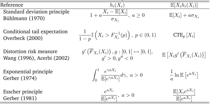
Other examples of risk measures of the formE[Xihi(Xi)]are the standard deviation

princi-ple, the Esscher principle and the exponential principle. These are summarised in Table 1. Defining the volumesviby

vi = E

[Xihi(Xi)]

Pn

j=1E[Xjhj(Xj)]

, i= 1, . . . , n, (49)

we find that the allocation principle (44) reduces to

Ki=

K

Pn

j=1E[Xjhj(Xj)]E

[Xihi(Xi)], i= 1, . . . , n, (50)

[image:15.595.90.520.464.677.2]

which is a special case of the proportional allocation principles discussed in Section 2.3.5.

Table 1:Business unit driven capital allocation

Reference hi(Xi) E[Xihi(Xi)]

Standard deviation principle

B¨uhlmann (1970) 1 +a

Xi−E[Xi]

σXi

, a≥0 E[Xi] +aσXi

Conditional tail expectation Overbeck (2000)

1 1−pI

Xi > FX−i1(p)

, p∈(0,1) CTEp[Xi]

Distortion risk measure Wang (1996), Acerbi (2002)

g0 FXi(Xi)

, g : [0,1]7→[0,1], g0>0, g00 <0 E

Xig0 FXi(Xi)

Exponential principle Gerber (1974)

Z 1

0

eγaXi

E[eγaXi]dγ, a >0

1

alnE

eaXi

Esscher principle Gerber (1981)

eaXi

E[eaXi_], a >0

E[XieaXi]

E[eaXi_]

3.2.3 Aggregate portfolio driven allocations

Let us now consider the case where

ζi=h(S), i= 1, . . . , n, (51)

with h being a non-negative and non-decreasing function such thatE[h(S)] = 1. In this case,

the states-of-the-world to which we assign the heaviest weights are those under which the ag-gregate portfolio performs worst. Therefore, we call such allocationsaggregate portfolio driven allocations. The allocation rule (34) can now be rewritten as

Ki=E[Xih(S)] +vi(K−E[Sh(S)]), i= 1, . . . , n. (52)

Hence, the capitalKi allocated to unitiis determined using a weighted expectation of the loss

Xi, with higher weights attached to states-of-the-world that involve a large aggregate loss S.

Notice that the allocation principle (52) can be reformulated as

Ki=E[Xi] +Cov[Xi, h(S)] +vi(K−E[Sh(S)]), i= 1, . . . , n. (53)

This means that the capital allocated to thei-th business unit is given by the sum of the expected loss E[Xi], a loading which depends on the covariance between the individual and aggregate

losses Xi and h(S), plus a term proportional to the volume of the business unit. A strong

positive correlation betweenXiandh(S), which reflects thatXi could be a substantial driver of

the aggregate loss S, produces a higher allocated capitalKi. Allocation principles of the form

(52) are closely related to the ‘Euler’ allocations proposed in Tasche (2004).

Using aggregate portfolio driven allocations might be appropriate when one wants to inves-tigate each individual portfolio’s contribution to the aggregate loss of the entire company. In other words, the company wishes to evaluate the subportfolio performances, e.g. the returns on the allocated capitals, in the presence of the other subportfolios. This can provide relevant information to the company within which it can further be used to evaluate either business expansions or reductions.

A particular choice of the random variableh(S)considered in (52) is given by

h(S) = I S > F −1

S (p)

1−FS F_S−1(p)

, i= 1, . . . , n, (54)

for somep∈(0,1). In this case, we find thatE[Xih(S)]andE[Sh(S)]transform into E[Xih(S)] =EXi

S > F_S−1(p)

, i= 1, . . . , n (55) and

E[Sh(S)] = CTEp[S], (56)

respectively. Furthermore, by taking

h(S) =S−_E[S], (57) we find

E[Xih(S)] = Cov[Xi, S], i= 1, . . . , n (58)

and

E[Sh(S)] = Var[S]. (59)

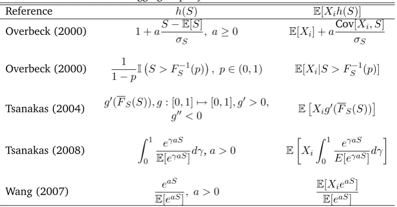
Other choices for the random variableh(S)and the related expressions for E[Xih(S)]can be

Defining the exposuresvi by

vi = E

[Xih(S)]

E[Sh(S)], i= 1, . . . , n, (60)

we find that the allocation principle (52) reduces to the proportional allocation rule

Ki =

K

E[Sh(S)]E[Xih(S)], i= 1, . . . , n. (61)

[image:17.595.106.500.267.472.2]

Now, the CTE allocation principle (23) that we discussed in Section 2.3.4 follows as a special case of the allocation principle (61) by choosing h(S) as in (54). Furthermore, takingh(S) as in (57) means that the allocation principle (61) effectively reduces to the covariance allocation principle (22) discussed in Section 2.3.3.

Table 2: Aggregate portfolio driven allocations

Reference h(S) E[Xih(S)]

Overbeck (2000) 1 +aS−E[S] σS

, a≥0 E[Xi] +a

Cov[Xi, S]

σS

Overbeck (2000) 1

1−pI S > F

−1

S (p)

, p∈(0,1) E[Xi|S > F_S−1(p)]

Tsanakas (2004) g 0_(F

S(S)), g: [0,1]7→[0,1], g0 >0,

g00<0 E

Xig0(FS(S))

Tsanakas (2008)

Z 1

0

eγaS

E[eγaS]dγ,a >0 E

Xi

Z 1

0

eγaS E[eγaS_]dγ

Wang (2007) e

aS

E[eaS], a >0

E[XieaS]

E[eaS]

3.2.4 Market driven allocations

LetζM be a random variable such that market-consistent values of the aggregate portfolio loss

S and the business unit lossesXi are given by

π[S] =E[ζMS] (62)

and

π[Xi] =E[ζMXi], i= 1, . . . , n, (63)

respectively. Further suppose that at the aggregate portfolio level, a provision π[S]is set aside to cover future liabilitiesS. Apart from the aggregate provisionπ[S], the aggregate portfolio has an available solvency capital equal to(K−π[S]). Thesolvency ratioof the aggregate portolio is then given by

K−π[S]

π[S] . (64)

In order to determine an optimal capital allocation over the different business units, we let in (31)ζi =ζM, i= 1, . . . , n, thus allowing the market to determine which states-of-the-world

are to be regarded adverse. This yields:

If we now use the market-consistent prices as volume measures, after substituting

vi =

π[Xi]

π[S], i= 1, . . . , n, (66) in (65), we find

Ki =

K

π[S]π[Xi], i= 1, . . . , n. (67) Rearranging these expressions leads to

Ki−π[Xi]

π[Xi]

= K−π[S]

π[S] , i= 1, . . . , n. (68) The quantitiesπ[Xi]and(Ki−π[Xi])can be interpreted as the market-consistent provision and

the solvency capital attached to business uniti, while Ki−π[Xi]

π[Xi] is its corresponding solvency ratio.

From (68), we can conclude that the optimisation criterion (33) withζi =ζM, i= 1, . . . , n, and

volume measures given by (66), leads to a capital allocation whereby the solvency ratio for each business unit is the same and equal to that of the aggregate portfolio. A similar allocation principle has been proposed by Sherris (2006) within the context of allocating the company’s total equity to the different business units “to determine an expected return on equity by line of business”.

3.2.5 Allocation with respect to the default option

An alternative choice for the weighting random variableζi is given by

ζi=h(S) = I

(S > K)

P[S > K], i= 1, . . . , n, (69)

such that only those states-of-the-world that correspond to insolvency are considered when de-termining the expectationsE[Xih(S)]. The allocation rule (34) then becomes

Ki =E[Xi |S > K] +vi(K−E[S|S > K]). (70)

Notice the similarity between (69) and the choice of h(S) made in (54) which led to the CTE allocation rule.

Expression (70) can be rearranged as follows:

E[(Xi−Ki)I(S > K)] =viE[(S−K)+], i= 1, . . . , n. (71) Summing the left and right hand sides of this expression overi= 1, . . . , n, leads to expression (29). The quantity E[(S−K)+]represents theexpected policyholder deficit or alternatively, the expected value of thedefault optionthat shareholders of an insurance company hold, given their limited liability. The allocation principle in (71) is such that the marginal contribution of each business unit to the expected value of the policyholder deficit is the same per unit of business volume, and hence is consistent with the arguments of Myers and Read Jr. (2001).

3.3 The absolute deviation optimisation criterion

In this section we discuss the optimal allocation problem under an absolute deviation criterion, that is, by letting

In this case the optimisation problem (31) reduces to

min

K1,...,Kn

n

X

j=1

E[ζj|Xj−Kj|],such that n

X

j=1

Kj =K. (73)

From the relation

|x|= 2 (x)₊−x, (74)

we immediately find that the optimal solution of (73) is identical to the solution of the following problem:

min

K1,...,Kn

n

X

j=1

Eζj(Xj−Kj)₊

, such that

n

X

j=1

Kj =K. (75)

This means that the absolute deviation optimisation problem (73) only takes into account the outcomes of the business unit lossesXj that lead to technical insolvencyXj > Kj in that unit.

In order to solve the optimisation problem (75), we first consider the special case where all

ζj’s are identical to 1.

Theorem 2 Assuming thatF_S−c1+(0)< K < F_S−c1(1), the optimal allocation problem

min

K1,...,Kn

n

X

j=1

E(Xj −Kj)₊

such that

n

X

j=1

Kj =K (76)

has the following solution:

Ki=F

−1(α)

Xi (FSc(K)), i= 1, . . . , n, (77)

whereScis defined in (10) andα∈[0,1]follows from

F_S−c1(α)(FSc(K)) =K. (78) Proof. Let α be determined from (78). Then we immediately find from Dhaene et al. (2002) that

E(Sc−K)₊ =

n X j=1 E

Xj−F

−1(α)

Xi (FSc(K)) + ≤ n X j=1

E(Xj−Kj)₊

, K ∈ F_S−c1+(0), F_S−c1(1)

,

holds for all(K1, K2, ..., Kn)such thatPn_j=1Kj =K. This proves the stated result.

We can conclude that the quantile allocation principle (14) considered in Section 2.3.2 is a solution of the minimisation problem (76). This optimisation problem and its solution were pre-viously considered in Dhaene et al. (2003) in the particular case that theFXi’s are all strictly

in-creasing. A proof of Theorem 2 using Lagrange techniques can be found in Laeven and Goovaerts (2004).

The solution to the general optimisation problem (73) will be expressed in terms of functions

F(ζi)

Xi defined as follows:

F(ζi)

One can prove that each function F(ζi)

Xi defines a proper distribution function, which we will

call the ζi–weighted distribution of Xi; see Rao (1997), Furman and Zitikis (2008a) and the

references therein. The decumulative distribution functionF(_Xζi_i)(x) = 1−F(ζi)

Xi (x)is given by

F(_Xζi_i)(x) =E[ζiI(Xi> x)] =E[ζi |Xi> x]FXi(x), i= 1, . . . , n. (80)

A sufficient condition forF(ζi)

Xi to be continuous is thatFXibe continuous. A sufficient condition

forF(ζi)

Xi to be strictly increasing is thatFXibe strictly increasing and thatP[ζi >0] = 1. For any

p∈(0,1)and anyα∈[0,1], we denote theα–mixed inverse ofF(ζi)

Xi at levelpby

F(ζi)

Xi

−1(α)

(p). In the following lemma, we prove that the deviation measureEζi(Xi−Ki)₊

can be trans-formed to a stop-loss premium of Xi with retention Ki, where the expectation is taken with

respect to theζi–weighted distribution ofXi.

Lemma 3 LetU be a uniform random variable on the unit interval(0,1). Then it holds that

Eζi(Xi−Ki)+

=E

F(ζi)

Xi −1

(U)−Ki

+

, i= 1, . . . , n. (81)

Proof. From the tower property of the expectation operator, we find

Eζi(Xi−Ki)+

=EζiE(Xi−Ki)+|ζi

.

SubstitutingE(Xi−Ki)₊|ζi

by

Z ∞

Ki

P[Xi > x|ζi]dxand changing the order of the

integra-tions, we find

Eζi(Xi−Ki)₊

=

Z ∞

Ki

E[ζi P[Xi> x|ζi]] dx

=

Z ∞

Ki

E[ζi E[I(Xi > x)|ζi]] dx.

Taking into account the tower property once more leads to

Eζi(Xi−Ki)₊

=

Z ∞

Ki

E[ζi I(Xi > x)] dx=

Z ∞

Ki

F(_Xζi_i)(x)dx.

The stated result follows then from observing that the distribution function of F(ζi)

Xi −1

(U)is given byF(ζi)

Xi so that

Z ∞

Ki

F(_Xζi_i)(x)dxis an expression for the stop-loss premium ofF(ζi)

Xi −1

(U) with retentionKi.

Now we are able to prove our main result concerning the absolute deviation optimisation problem.

Theorem 4 LetScbe the comonotonic sum defined by

Sc=

n

X

i=1

F(ζi)

Xi −1

where the random variableU is uniformly distributed on the unit interval(0,1). In caseF−1+

Sc (0)<

K < F−1

Sc (1), the optimal allocation problem (73) has the following solution:

Ki=

F(ζi)

Xi

−1(α)

(F_ScK), i= 1, . . . , n, (83)

whereα∈[0,1]follows from

F−1(α)

Sc (FSc(K)) =K. (84)

Proof. From Lemma 3, we find that the optimisation problem (73) can be rewritten as

min

K1,...,Kn

n

X

j=1

E

F(ζj)

Xj −1

(U)−Kj

+

, such that

n

X

j=1

Kj =K.

The stated result follows then by applying Theorem 2.

From the theorem above, we can conclude that the mean absolute deviation optimality crite-rion (73) gives rise to a quantile-based allocation principle: Each allocated capitalKiis given by

theα–mixed inverse of theζi–weighted distribution function ofXi at a fixed probability level,

which is chosen such that the full allocation requirement is satisfied. From (83), we find that the optimal allocationsKisatisfy the following conditions:

F(ζi)

Xi (Ki) =FS

c(K), i= 1, . . . , n. (85)

In the case where

P[ζi >0] = 1, i= 1, . . . , n, (86)

and the distributionsF(ζj)

Xj are strictly increasing, then the optimal allocations in (83) reduce to

Ki=

F(ζi)

Xi −1

(F_ScK), i= 1, . . . , n. (87)

We end this subsection with an example of an absolute deviation allocation principle. Con-sider the following choice for the weighting random variables:

ζi = I

(S > K)

P[S > K], i= 1, . . . , n. (88)

This means that the optimisation procedure only considers those outcomes that lead to insol-vency, i.e. the case whereS > K, on the aggregate portfolio level. In this instance, the optimi-sation problem (75) reduces to

min

K1,...,Kn

n

X

j=1

E(Xj−Kj)₊|S > K

, such that

n

X

j=1

Kj =K. (89)

From (79), we find that theζi–weighted distribution function ofXiis given by

F(ζi)

Xi (x) =P[Xi≤x|S > K], i= 1, . . . , n. (90)

In the particular case thatx=Ki, we find from (85) that:

F(_Xζi_i)(Ki) =P[Xi > Ki|S > K] =FSc(K), i= 1, . . . , n. (91)

4

Conclusion

In this article, we developed a general and unifying optimisation framework that produces sev-eral of the capital allocation approaches that are encountered both in the literature and in practice. This general framework is based on the idea of minimising the sum of the divergences between the losses and the allocated capital of the different subportfolios.

Depending on how this divergence is defined, several alternative allocation methods arise. In particular, choice of the functionsζi determines which scenarios (states of the world), e.g.

port-folio or unit-specific, carry most weight in the capital allocation. We believe that this approach allows for a closer alignment between capital allocation and the definition of management’s risk tolerance.

Finally, the framework presented in this paper provides the flexibility to produce new capital allocation methods, by varying, for example, the choices of the weightsζi andvi. This is not an

avenue we pursued here at great lengths but remains a subject of importance for future work.

Acknowledgement:The authors thank Qihe Tang, Yaniv Zaks and Peter England for their helpful com-ments and suggestions on an earlier version of this paper. Jan Dhaene acknowledges the financial support of the Onderzoeksfonds K.U. Leuven (GOA/07: Risk Modeling and Valuation of Insurance and Financial Cash Flows, with Applications to Pricing, Provisioning and Solvency), and of Fortis through the K.U. Leuven Fortis Chair in Financial and Actuarial Risk Management.

References

C. Acerbi. Spectral measures of risk: a coherent representation of subjective risk aversion. Journal of Banking and Finance, 26(7):1505–1518, 2002.

C. Acerbi and D. Tasche. On the coherence of expected shortfall.Journal of Banking and Finance, 26(7):1487–1503, 2002.

P. Artzner, F. Delbaen, J.-M. Eber, and D. Heath. Coherent measures of risk. Mathematical Finance, 9(3):203–228, 1999.

H. B¨uhlmann. Mathematical Methods in Risk Theory. Springer-Verlag, Berlin, 1970.

J.D. Cummins. Allocation of capital in the insurance industry. Risk Management and Insurance Review, 3(1):7–27, 2000.

M. Denault. Coherent allocation of risk capital. Journal of Risk, 4(1):1–34, 2001.

J. Dhaene, M. Denuit, M.J. Goovaerts, R. Kaas, and D. Vyncke. The concept of comonotonicity in actuarial science and finance: theory. Insurance: Mathematics and Economics, 31:3–33, 2002.

J. Dhaene, M.J. Goovaerts, and R. Kaas. Economic capital allocation derived from risk measures. North American Actuarial Journal, 7(2):44–59, 2003.

J. Dhaene, S. Vanduffel, Q. Tang, M.J. Goovaerts, R. Kaas, and D. Vyncke. Risk measures and comonotonicity: a review. Stochastic Models, 22(4):573–606, 2006.

J. Dhaene, L. Henrard, Z. Landsman, A. Vandendorpe, and S. Vanduffel. Some results on the CTE based capital allocation rule. Insurance: Mathematics and Economics, 42(2):855–863, 2008.

H. F¨ollmer and A. Schied. Convex measures of risk and trading constraints.Finance and Stochas-tics, 6(4):429–447, 2002.

E. Furman and R. Zitikis. Weighted premium calculation principles. Insurance: Mathematics and Economics, 42(1):459–465, 2008a.

E. Furman and R. Zitikis. Weighted risk capital allocations. Insurance: Mathematics and Eco-nomics, 43(2):263–269, 2008b.

H.U. Gerber. On additive premium calculation principles. ASTIN Bulletin, 7(3):215–222, 1974.

H.U. Gerber. The Esscher premium principle: a criticism. comment. ASTIN Bulletin, 12(2): 139–140, 1981.

M.J. Goovaerts, F. deVylder, and J. Haezendonck. Insurance Premiums: Theory and Applications. Amsterdam, North Holland, 1984.

H. Gr¨undl and H. Schmeiser. Capital allocation for insurance companies: what good is it? Journal of Risk and Insurance, 74(2):301–317, 2007.

W.R. Heilmann. Decision theoretic foundations of credibility theory. Insurance: Mathematics and Economics, 8:77–95, 1989.

M. Kalkbrener. An axiomatic approach to capital allocation. Mathematical Finance, 15(3):425– 437, 2005.

J. Kim and M. Hardy. A capital allocation based on a solvency exchange option. Insurance: Mathematics and Economics, 2008. In press.

R.J.A. Laeven and M.J. Goovaerts. An optimization approach to the dynamic allocation of eco-nomic capital. Insurance: Mathematics and Economics, 35(2):299–319, 2004.

Z. Landsman and E.A. Valdez. Tail conditional expectations for elliptical distributions. North American Actuarial Journal, 7(4):55–71, 2003.

J. LeMaire. An application of game theory: cost allocation. ASTIN Bulletin, 14(1):61–81, 1984.

S.C. Myers and J.A. Read Jr. Capital allocation for insurance companies. Journal of Risk and Insurance, 68(4):545–580, 2001.

L. Overbeck. Allocation of economic capital in loan portfolios. in J. Franke, W. Haerdle and G. Stahl (eds.), Measuring Risk in Complex Systems, Springer, 2000.

H.H. Panjer. Measurement of risk, solvency requirements, and allocation of capital within fi-nancial conglomerates. Research Report 01-14. Institute of Insurance and Pension Research, University of Waterloo, Canada, 2001.

R.D. Phillips, J.D. Cummins, and F. Allen. Financial pricing of insurance in the multiple-line insurance company. Journal of Risk and Insurance, 65(4):597–636, 1998.

C.R. Rao. Statistics and Truth: Putting Chance to Work. World Scientific Publishing, River Edge, NJ, 1997.

D. Tasche. Allocating portfolio economic capital to sub-portfolios. In A. Dev (ed.), Economic Capital: A Practitioner’s Guide, Risk Books, pp. 275-302, 2004.

A. Tsanakas. Dynamic capital allocation with distortion risk measures. Insurance: Mathematics and Economics, 35(2):223–243, 2004.

A. Tsanakas. Capital allocation with risk measures. Proceedings of the 5th Actuarial and Finan-cial Mathematics Day, 9 February, Brussels, pp. 3-17, 2007.

A. Tsanakas. To split or not to split: capital allocation with convex risk measures. Insurance: Mathematics and Economics, 2008. In press.

E.A. Valdez and A. Chernih. Wang’s capital allocation formula for elliptically contoured distri-butions. Insurance: Mathematics and Economics, 33(3):517–532, 2003.

G.G. Venter. Capital allocation survey with commentary. North American Actuarial Journal, 8 (2):96–107, 2004.

S.S. Wang. Premium calculation by transforming the premium layer density. ASTIN Bulletin, 26 (1):71–92, 1996.

S.S. Wang. Normalized exponential tilting: pricing and measuring multivariate risks. North American Actuarial Journal, 11(3):89–99, 2007.