Convergence rates of the truncated Euler-Maruyama method for stochastic differential equations

Convergence Rates of the Truncated

Euler–Maruyama Method for Stochastic Differential

Equations

Xuerong Mao∗

Department of Mathematics and Statistics, University of Strathclyde, Glasgow G1 1XH, U.K.

Abstract

Influenced by Higham, Mao and Stuart [9], several numerical methods have been de-veloped to study the strong convergence of the numerical solutions to stochastic differen-tial equations (SDEs) under the local Lipschitz condition. These numerical methods in-clude the tamed Euler–Maruyama (EM) method, the tamed Milstein method, the stopped EM, the backward EM, the backward forward EM, etc. Recently, we developed a new explicit method in [23], called the truncated EM method, for the nonlinear SDE dx(t) = f(x(t))dt+g(x(t))dB(t) and established the strong convergence theory under the local Lip-schitz condition plus the Khasminskii-type condition xT_{f(x) +} p−1

2 |g(x)|

2 _{≤ K(1 +|x|}2_).

However, due to the page limit there, we did not study the convergence rates for the method, which is the aim of this paper. We will, under some additional conditions, discuss the rates of Lq_{-convergence of the truncated EM method for 2≤q < p and show that the order of}

Lq_{-convergence can be arbitrarily close toq/2.}

Key words: Stochastic differential equation, local Lipschitz condition, Khasminskii-type condition, truncated Euler-Maruyama method, convergence rate.

1

Introduction

This is the continuation of our recent paper [23], where we developed a new explicit method, called the truncated EM method, for the multi-dimensional nonlinear SDE

dx(t) =f(x(t))dt+g(x(t))dB(t)

and established the strong convergence theory under the local Lipschitz condition plus the Khasminskii-type condition

xTf(x) +p−1 2 |g(x)|

2 _{≤K(1 +|x|}2_).

However, we did not study the convergence rates for the method there. The key aim of this paper is to discuss the rates ofLq-convergence for 2≤q < p.

In [23], we have reviewed the developments of numerical methods for SDEs for the past twenty years. In summary, up to 2002, most of the existing strong convergence theory for numerical methods requires the coefficients of the SDEs to be globally Lipschitz continuous (see, e.g., [18, 21, 27]). In 2002, Higham, Mao and Stuart published a very influential paper [9] (Google citation 318 on 6 September 2015) which opened a new chapter in the study of numerical

∗

solutions of SDEs—to study the strong convergence question for numerical approximations under the local Lipschitz condition. For example, implicit methods have been used to study the numerical solutions to SDEs without the linear growth condition (see, e.g., [24, 34, 35] and for the background on the implicit methods, we refer the reader to the papers [2, 4, 9, 12, 11, 17, 26, 31] and the book [18]). Methods with variable stepsize also attract a lot of attention [5, 29, 36, 39]. Other weak forms of convergence, say weak convergence, convergence in probability and pathwise convergence, are discussed in [1, 7, 16, 18, 22, 25, 28, 37], just to mention a few. More significantly, some modified EM methods have recently been developed for the nonlinear SDEs without the linear growth condition. For example, the tamed EM method was developed in [14] to approximate SDEs with one-sided Lipschitz drift coefficient and the linear growth diffusion coefficient. This method was further developed in [33] while the tamed Milstein method was developed in [38]. Moreover, the stopped EM method was developed in [20] for nonlinear SDEs as well. Very recently, another new explicit method—the truncated EM method was developed in [23]. These new explicit EM methods have shown their abilities to approximate the solutions of nonlinear SDEs.

In this paper, we will investigate the convergence rates of the truncated EM method. For the convenience of the reader, we will, in section 2, make a quick review on the main results in [23], where the truncated EM method was initiated. We will then study the rates of convergence at a single time in section 3 and over a finite time interval in section 4. A number of examples will be discussed throughout sections 3 and 4 to illustrate our theory and to motivate further developments. We will conclude our paper in section 5.

2

The Truncated EM Method

Throughout this paper, unless otherwise specified, we let (Ω,F,P) be a complete probability

space with a filtration{F_t}_t≥0 satisfying the usual conditions (that is, it is right continuous and increasing whileF0 contains all P-null sets), and let Edenote the expectation corresponding to P. Let B(t) be an m-dimensional Brownian motion defined on the space. If A is a vector or

matrix, its transpose is denoted by AT. If x ∈ _Rd_{, then |x| is the Euclidean norm. If A is a}

matrix, we let |A|= ptrace(AT_{A) be its trace norm. If A is a symmetric matrix, denote by}

λmax(A) and λmin(A) its largest and smallest eigenvalue, respectively. Moreover, for two real

numbers a and b, we use a∨b = max(a, b) and a∧b = min(a, b). If G is a set, its indicator function is denoted byIG, namely IG(x) = 1 if x∈G and 0 otherwise.

Consider a d-dimensional SDE

dx(t) =f(x(t))dt+g(x(t))dB(t) (2.1)

on t≥0 with the initial value x(0) =x0∈Rd, where

f :Rd→Rd and g:Rd→Rd×m.

We impose two standing hypotheses in this paper.

Assumption 2.1 Assume that the coefficientsf andgsatisfy the local Lipschitz condition: For anyR >0, there is aKR>0 such that

|f(x)−f(y)| ∨ |g(x)−g(y)| ≤KR|x−y| (2.2)

Assumption 2.2 We also assume that the coefficients satisfy the Khasminskii-type condition: There is a pair of constants p >2 and K >0 such that

xTf(x) + p−1 2 |g(x)|

2 _{≤K(1 +|x|}2_{) (2.3)}

for all x∈Rd.

We state a known result (see, e.g., [21, 22, 32]) as a lemma for the use of this paper.

Lemma 2.3 Under Assumptions 2.1 and 2.2, the SDE (2.1) has a unique global solution x(t) and, moreover,

sup

0≤t≤TE

|x(t)|p <∞, ∀T >0. (2.4)

Let us now review the truncated EM method initiated in [23]. To define the truncated EM numerical solutions, we first choose a strictly increasing continuous function µ:R+→R+ such

thatµ(u)→ ∞ asu→ ∞and

sup |x|≤u

|f(x)| ∨ |g(x)|

≤µ(u), ∀u≥1. (2.5)

Denote by µ−1 the inverse function ofµand we see that µ−1 is a strictly increasing continuous function from [µ(0),∞) to R+. We also choose a number ∆∗ ∈(0,1] and a strictly decreasing

functionh: (0,∆∗]→(0,∞) such that

h(∆∗)≥µ(2), lim

∆→0h(∆) =∞ and ∆

1/4_{h(∆)≤1, ∀∆∈(0,∆}∗_{]. (2.6)}

For a given stepsize ∆∈(0,∆∗], let us define the truncated functions

f∆(x) =f

(|x| ∧µ−1(h(∆))) x

|x|

and g∆(x) =g

(|x| ∧µ−1(h(∆))) x

|x|

(2.7)

forx∈_Rd_{, where we set x/|x|= 0 when x= 0. It is easy to see that}

|f∆(x)| ∨ |g∆(x)| ≤µ(µ−1(h(∆))) =h(∆), ∀x∈Rd. (2.8)

That is, both truncated functions f∆ and g∆ are bounded although bothf and g may not. It

was shown in [23] that these truncated functions preserve nicely the Khasminskii-type condition for all ∆∈(0,∆∗] as described in the following lemma.

Lemma 2.4 Let Assumption 2.2 hold. Then, for all ∆∈(0,∆∗], we have

xTf∆(x) +

p−1

2 |g∆(x)|

2 _{≤2K(1 +|x|}2_{), ∀x∈}

Rd. (2.9)

The discrete-time truncated EM numerical solutionsX∆(tk)≈x(tk) fortk =k∆ are formed

by settingX∆(0) =x0 and computing

X∆(tk+1) =X∆(tk) +f∆(X∆(tk))∆ +g∆(X∆(tk))∆Bk, (2.10)

fork= 0,1,· · ·, where ∆Bk =B(tk+1)−B(tk). There are two versions of the continuous-time

truncated EM solutions. The first one is defined by

¯ x∆(t) =

∞

X

k=0

This is a simple step process so its sample paths are not continuous. We will refer this as the continuous-time step-process truncated EM solution. The other one is defined by

x∆(t) =x0+

Z t

0

f∆(¯x∆(s))ds+

Z t

0

g∆(¯x∆(s))dB(s) (2.12)

fort ≥0. We will refer this as the continuous-time continuous-sample truncated EM solution. We observe that x∆(tk) = ¯x∆(tk) = X∆(tk) for all k ≥ 0. Moreover, x∆(t) is an Itˆo process

with its Itˆo differential

dx∆(t) =f∆(¯x∆(t))dt+g∆(¯x∆(t))dB(t). (2.13)

The truncated EM solutions have a number of nice properties established in [23]. We will cite a number of them here for the use of this paper.

Lemma 2.5 For any ∆∈(0,∆∗]and any p >ˆ 0, we have

E|x∆(t)−x¯∆(t)|pˆ≤cpˆ∆p/ˆ 2(h(∆))pˆ, ∀t≥0, (2.14)

where cpˆ is a positive constant dependent only on pˆ. Consequently

lim

∆→0E|x∆(t)−x¯∆(t)|

ˆ

p _{= 0, ∀t≥0. (2.15)}

It should be pointed out that this lemma was proved only for ˆp ≥2 in [23]. However, it is easy to see that this lemma holds for any ˆp ∈(0,2) as well. In fact, by the H¨older inequality, for any ˆp∈(0,2), we have

E|x∆(t)−x¯∆(t)|pˆ≤

E|x∆(t)−x¯∆(t)|2

p/ˆ 2

≤c2∆(h(∆))2

p/ˆ2

=cpˆ∆p/ˆ 2(h(∆))pˆ

as desired. This is useful as in our proofs later we will use this lemma for any ˆp >0. For example, in the proof of Lemma 3.3, this lemma will be applied on the expressionE|x∆(t)−x¯∆(t)|pq/(2p−pr)

in (3.10) and our conditions there only ensure that pq/(2p−pr)>0.

Lemma 2.6 Let Assumptions 2.1 and 2.2 hold. Then

sup

0<∆≤∆∗_0≤sup_t≤TE

|x∆(t)|p ≤C, ∀T >0, (2.16)

where, and from now on, C stands for generic positive real constants dependent on T, p, K, x0

etc. but independent of ∆,R (appeared in the next lemmas) and its values may change between occurrences.

Lemma 2.7 Let Assumptions 2.1 and 2.2 hold. For any real number R > |x0|, define the

stopping time

τR= inf{t≥0 :|x(t)| ≥R},

where throughout this paper we setinf∅=∞ (and as usual ∅ denotes the empty set). Then

P(τR≤T)≤

C

Rp. (2.17)

Lemma 2.8 Let Assumptions 2.1 and 2.2 hold. For any real numberR >|x0|and∆∈(0,∆∗),

define the stopping time

ρ∆,R = inf{t≥0 :|x∆(t)| ≥R}.

Then

P(ρ∆,R ≤T)≤

C

3

Convergence Rates at Time

T

In [23], we established the theory of the strong Lq-convergence for 2 ≤ q < p, where p is a parameter in Assumption 2.2. However, the convergence was in the asymptotic form without the convergence rate. Starting from this section we will discuss the convergence rate. Our study on the convergence rate will also reveal a strong relation between functions µ(·) and h(·) that are used to define the truncated EM method. We first discuss the convergence rate at time T in this section and then discuss the path convergence rate in the next section. We need some additional conditions.

Assumption 3.1 Assume that there is a pair of constantsq ≥2 and H1>0 such that

(x−y)T(f(x)−f(y)) + q−1

2 |g(x)−g(y)|

2 _≤H

1|x−y|2 (3.1)

for all x, y∈_Rd_.

Assumption 3.2 Assume that there is a pair of positive constantsr and H2 such that

|f(x)| ≤H2(1 +|x|r), ∀x∈Rd. (3.2)

The following lemma will play a key role in the proof of the convergence rate.

Lemma 3.3 Let Assumptions 2.1, 2.2, 3.1 and 3.2 hold and assume that 2p > qr and p > q. LetR >|x0|be a real number and let ∆∈(0,∆∗)be sufficiently small such thatµ−1(h(∆))≥R.

Let τR andρ∆,R be the same as defined in Lemmas 2.7 and 2.8, respectively. Set

θ∆,R =τR∧ρ∆,R and e∆(t) =x∆(t)−x(t) for t≥0.

Then

E|e∆(T∧θ∆,R)|q≤C∆q/4(h(∆))q/2, ∀T >0. (3.3)

Proof. We write θ∆,R = θ for simplicity. By the Itˆo formula [21, 30], we can show that for

0≤t≤T,

E|e∆(t∧θ)|q

≤ _E

Z t∧θ

0

q|e∆(s)|q−2

eT_∆(s)[f(x(s))−f∆(¯x∆(s))] +

q−1

2 |g(x(s))−g∆(¯x∆(s))|

2_{ds. (3.4)}

We observe that for 0 ≤ s ≤ t∧θ, |x¯∆(s)| ≤ R. But we have condition µ−1(h(∆)) ≥ R, so |x¯∆(s)| ≤µ−1(h(∆)). Recalling the definition of the truncated functions f∆ and g∆, we hence

have that

f∆(¯x∆(s)) =f(¯x∆(s)) and g∆(¯x∆(s)) =g(¯x∆(s)) for 0≤s≤t∧θ.

It therefore follows from (3.4) that

E|e∆(t∧θ)|q

≤ _E

Z t∧θ

0

q|e∆(s)|q−2

eT_∆(s)[f(x(s))−f(¯x∆(s))] +

q−1

2 |g(x(s))−g(¯x∆(s))|

2_{ds. (3.5)}

Re-arranging this gives

where

J1 =E Z t∧θ

0

q|e∆(s)|q−2

(x(s)−x¯∆(s))T[f(x(s))−f(¯x∆(s))]

+q−1

2 |g(x(s))−g(¯x∆(s))|

2_{ds (3.7)}

and

J2 =E Z t∧θ

0

q|e∆(s)|q−2(¯x∆(s)−x∆(s))T[f(x(s))−f(¯x∆(s))]ds. (3.8)

By Assumption 3.1, the Young inequality and Lemma 2.5, we derive that

J1 ≤ qH1E Z t∧θ

0

|e∆(s)|q−2|x(s)−x¯∆(s)|2ds

≤ 2qH1E Z t∧θ

0

|e∆(s)|q+|e∆(s)|q−2|x∆(s)−x¯∆(s)|2

ds

≤ 4(q−1)H1E Z t∧θ

0

|e∆(s)|qds+ 4H1E Z t∧θ

0

|x∆(s)−x¯∆(s)|qds

≤ 4(q−1)H1

Z t

0

E|e∆(s∧θ)|qds+ 4H1

Z T

0

E|x∆(s)−x¯∆(s)|qds

≤ 4(q−1)H1

Z t

0

E|e∆(s∧θ)|qds+C∆q/2(h(∆))q. (3.9)

Moreover, by Assumption 3.2 and the H¨older inequality as well as Lemmas 2.3, 2.5 and 2.6, we derive that

J2 ≤ E Z t∧θ

0

(q−2)|e∆(s)|q+ 2|x¯∆(s)−x∆(s)|q/2|f(x(s))−f(¯x∆(s))|q/2

ds

≤ (q−2)E Z t

0

|e∆(s∧θ)|qds

+ C

Z T

0

E

|x¯∆(s)−x∆(s)|q/2(1 +|x(s)|qr/2+|x¯∆(s)|qr/2)

ds

≤ (q−2)

Z t

0

E|e∆(s∧θ)|qds

+ C

Z T

0

E|x¯∆(s)−x∆(s)|pq/(2p−qr)

(2p−qr)/2p

(1 +E|x(s)|p+E|x¯∆(s)|p)

qr/2p

ds

≤ (q−2)

Z t

0

E|e∆(s∧θ)|qds+C∆q/4(h(∆))q/2. (3.10)

Substituting (3.9) and (3.10) into (3.6) yields

E|e∆(t∧θ)|q ≤C

Z t

0

E|e∆(s∧θ)|qds+C∆q/4(h(∆))q/2.

By the Gronwall inequality, we obtain the required assertion (3.3). 2

Let us now state our first result on the convergence rate, where we reveal a strong relation between functions µ(·) and h(·), which are used to define the truncated EM method.

Theorem 3.4 Let Assumptions 2.1, 2.2, 3.1 and 3.2 hold with 2p > qr and p > q. If

h(∆)≥µ (∆q/4(h(∆))q/2)−1/(p−q)

for all sufficiently small ∆∈(0,∆∗), then, for every such small ∆,

E|x(T)−x∆(T)|q≤C∆q/4(h(∆))q/2 and E|x(T)−x¯∆(T)|q ≤C∆q/4(h(∆))q/2 (3.12)

for all T >0.

Proof. Let τR, ρ∆,R, θ∆,R and e∆(t) be the same as before. Using the Young inequality, we

derive that for any δ >0,

E|e∆(T)|q = E

|e∆(T)|qI{θ∆,R>T}

+E

|e∆(T)|qI{θ∆,R≤T}

≤ E

|e∆(T)|qI{θ∆,R>T}

+qδ

pE|e∆(T)|

p₊ p−q

pδq/(p−q)P(θ∆,R≤T). (3.13)

By Lemmas 2.3 and 2.6, we have

E|e∆(T)|p ≤C

while by Lemmas 2.7 and 2.8,

P(θ∆,R ≤T)≤P(τR≤T) +P(ρ∆,R ≤T)≤

C Rp.

We hence have

E|e∆(T)|q ≤E

|e∆(T)|qI{θ∆,R>T}

+Cqδ p +

C(p−q)

pRpδq/(p−q). (3.14)

Consequently

E|e∆(T)|q≤E

|e∆(T ∧θ∆,R)|q

+ Cqδ p +

C(p−q)

pRpδq/(p−q) (3.15)

holds for any ∆∈(0,∆∗),R >|x0|and δ >0. We can therefore choose δ= ∆q/4(h(∆))q/2 and

R= (∆q/4(h(∆))q/2)−1/(p−q) to get

E|e∆(T)|q≤E|e∆(T ∧θ∆,R)|q+C∆q/4(h(∆))q/2. (3.16)

But, by condition (3.11), we have

µ−1(h(∆))≥(∆q/4(h(∆))q/2)−1/(p−q) =R.

We can hence apply Lemma 3.3 to obtain

E|e∆(T ∧θ∆,R)|q ≤C∆q/4(h(∆))q/2. (3.17)

Substituting this into (3.16) yields the first inequality in (3.12). The second inequality there follows from the first one and Lemma 2.5. 2

Example 3.5 Let us illustrate this theorem by an example before we discuss a better conver-gence rate under stronger conditions. Consider the scalar SDE

dx(t) = (x(t)−x3(t))dt+|x(t)|3/2dB(t), (3.18)

where B(t) is a scalar Brownian motion. This is a specified Lewis stochastic volatility model [19]. The reason we only consider this specified model is to keep it simple while our theory is illustrated fully. Of course, our theory works for the general Lewis stochastic volatility model. Clearly, its coefficients f(x) = x−x3 and g(x) = |x|3/2 _{are locally Lipschitz continuous (i.e.,}

satisfy Assumption 2.1). Also, for anyp >3, we have

xf(x) +p−1 2 |g(x)|

2_=|x|2_{− |x|}4₊p−1

2 |x|

which is bounded above, say byK, forx∈_R. That is, Assumption 2.2 is satisfied for anyp >3. Moreover, by the mean-value theorem, it is easy to show that

|g(x)−g(y)| ≤ 3

2(|x|

1/2_+|y|1/2_{)|x−y|, ∀x, y∈}

R. (3.19)

We can then further show that

(x−y)(f(x)−f(y)) + 1

2|g(x)−g(y)|

2 _≤4|x−y|2_.

In other words, Assumption 3.1 is satisfied withq = 2. Furthermore, it is obvious that

|f(x)| ≤ |x|+|x|3 ≤2(1 +|x|3), ∀x∈_R.

Namely, Assumption 3.2 holds with r = 3. So far, we have verified that Assumptions 2.1, 2.2, 3.1, 3.2 hold for q = 2, r = 3 and any p > 3. To apply Theorem 3.4, we still need to design functions µand h in order for (3.11) to hold for all sufficiently small ∆. Noting that

sup |x|≤u

(|f(x)| ∨ |g(x)|)≤2u3, ∀u≥1,

we can have µ(u) = 2u3 and its inverse function µ−1(u) = (u/2)1/3 foru ≥0. Forε∈(0,1/4], we define h(∆) = ∆−ε _{for ∆ >0. Letting ∆}∗ _{∈(0,1] be sufficiently small, we can make (2.6)} hold. Now, inequality (3.11) becomes

∆−ε≥2(∆1/2−ε)−3/(p−2), namely, 1≥2∆ε−3(1/2−ε)/(p−2). (3.20)

But, for any ε∈(0,1/4], we can choose sufficiently largep such thatε−3(1/2−ε)/(p−2)>0 and hence (3.20) holds for all sufficiently small ∆. We can therefore conclude by Theorem 3.4 that the truncated EM solutions of the SDE (3.18) satisfy

E|x(T)−x∆(T)|2=O(∆1/2−ε) and E|x(T)−x¯∆(T)|2=O(∆1/2−ε).

This example shows that when the truncated EM method is applied to the SDE (3.18), the order ofL2-convergence is close to 1/2 (or, the order ofL1-convergence is close to 1/4). Can we improve the order?

The answer is yes. In the remaining of this section, we will establish a new result which shows the order of Lq-convergence is close to q/2. This is almost optimal if we recall that the classical EM method has orderq/2 ofLq-convergence under the global Lipschitz condition. For this almost optimal result, we need slightly stronger condition than Assumption 3.2.

Assumption 3.6 Assume that there is a pair of positive constantsρ and H3 such that

|f(x)−f(y)|2∨ |g(x)−g(y)|2≤H3(1 +|x|ρ+|y|ρ)|x−y|2 (3.21)

for all x, y∈_Rd_.

The following is another key lemma.

Lemma 3.7 Let Assumptions 2.1, 2.2, 3.1 and 3.6 hold and assume thatp > q >2and2p > qρ. LetR >|x0|be a real number and let ∆∈(0,∆∗)be sufficiently small such thatµ−1(h(∆))≥R.

Let θ∆,R and e∆(t) be the same as before. Then, for anyq¯∈[2, q),

Proof. We use the same notation as in the proof of Lemma 3.3. Clearly, (3.5) holds when q there is replaced with ¯q. Namely, we have

E|e∆(t∧θ)|q¯

≤ _E

Z t∧θ

0

¯

q|e∆(s)|q¯−2

eT_∆(s)[f(x(s))−f(¯x∆(s))] +

¯ q−1

2 |g(x(s))−g(¯x∆(s))|

2_{ds. (3.23)}

Noting

¯ q−1

2 |g(x(s))−g(¯x∆(s))|

2

≤ q¯−1

2

h

1 +q−q¯ ¯ q−1

|g(x(s))−g(x∆(s))|2+

1 +q¯−1 q−q¯

|g(x∆(s))−g(¯x∆(s))|2

i

= q−1

2 |g(x(s))−g(x∆(s))|

2₊(¯q−1)(q−1)

2(q−q¯) |g(x∆(s))−g(¯x∆(s))|

2_,

we get from (3.23) that

E|e∆(t∧θ)|q¯≤J3+J4, (3.24)

where

J3=E Z t∧θ

0

¯

q|e∆(s)|q¯−2

eT_∆(s)[f(x(s))−f(x∆(s))] +

q−1

2 |g(x(s))−g(x∆(s))|

2_{ds (3.25)}

and

J4 =E Z t∧θ

0

¯

q|e∆(s)|q¯−2

eT_∆(s)[f(x∆(s))−f(¯x∆(s))]

+(¯q−1)(q−1)

2(q−q¯) |g(x∆(s))−g(¯x∆(s))|

2_{ds. (3.26)}

By Assumption 3.1, we can show easily that

J3≤qH¯ 1

Z t

0

E|e∆(s∧θ)|q¯ds. (3.27)

By Assumption 3.6, we also have

J4≤(¯q/2)

Z t

0

E|e∆(s∧θ)|q¯ds+J5, (3.28)

where

J5 =CE Z t∧θ

0

|e∆(s)|q¯−2(1 +|x∆(s)|ρ+|x¯∆(s)|ρ)|x∆(s)−x¯∆(s)|2

ds.

By the Young inequality etc., we derive that

J5 ≤ C

Z t

0

E|e∆(s∧θ)|q¯ds

+ C

Z T

0

E

(1 +|x∆(s)|ρq/¯ 2+|x¯∆(s)|ρq/¯2)|x∆(s)−x¯∆(s)|q¯

ds. (3.29)

In the same way as (3.10) was proved, we can then show

J5 ≤ C

Z t

0

Putting (3.30) into (3.28) and then substituting it and (3.27) into (3.24), we get

E|e∆(t∧θ)|q¯≤C

Z t

0

E|e(s∧θ)|q¯ds+C∆q/¯2(h(∆))q¯.

By the Gronwall inequality, we obtain the required assertion (3.22). 2

The following theorem shows a higher order ofLq¯-convergence of the truncated EM method.

Theorem 3.8 Let Assumptions 2.1, 2.2, 3.1 and 3.6 hold with p > q > 2 and 2p > qρ. Let ¯

q∈[2, q). If

h(∆)≥µ [∆¯q/2(h(∆))q¯]−1/(p−q¯)

(3.31)

for all sufficiently small ∆∈(0,∆∗), then, for every such small ∆,

E|x(T)−x∆(T)|q¯≤C∆q/¯ 2(h(∆))q¯ and E|x(T)−x¯∆(T)|2≤C∆q/¯ 2(h(∆))q¯. (3.32)

Proof. We use the same notation as in the proof of Theorem 3.4. Clearly, (3.15) holds ifq there is replaced with ¯q. Choosingδ = ∆q/¯2(h(∆))q¯and R= [∆q/¯2(h(∆))q¯]−1/(p−q¯), we then obtain

E|e∆(T)|q¯≤E|e∆(T∧θ∆,R)|q¯+C∆q/¯ 2(h(∆))q¯. (3.33)

But, by condition (3.31), we have

µ−1(h(∆))≥[∆q/¯2(h(∆))q¯]−1/(p−q¯)=R.

We can hence apply Lemma 3.7 to obtain

E|e∆(T∧θ∆,R)|q¯≤C∆q/¯2(h(∆))q¯. (3.34)

Substituting this into (3.33) yields the first inequality in (3.32). The second inequality there follows from the first one and Lemma 2.5. 2

Example 3.9 (Continuation of Example 3.5) Let us now return to the SDE (3.18). Re-calling (3.19), we can easily show that, for anyx, y∈_R,

(x−y)(f(x)−f(y)) +|g(x)−g(y)|2 ≤12|x−y|2

and

|f(x)−f(y)|2∨ |g(x)−g(y)|2 ≤12(1 +|x|4+|y|4)|x−y|2.

In other words, Assumptions 3.1 and 3.6 are satisfied with q = 3 and ρ = 4. We hence have that Assumptions 2.1, 2.2, 3.1, 3.6 hold for q= 3,ρ= 4 and any p >6. To apply Theorem 3.8, we let ¯q = 2 and still chooseµ(u) = 2u3 _{but leth(∆) = ∆}−ε/2 _{forε∈(0,1/2]. Then, inequality}

(3.31) becomes

∆−ε/2 ≥2∆−3(1−ε)/(p−2), namely, 1≥2∆ε/2−3(1−ε)/(p−2). (3.35)

But, for anyε∈(0,1/2], we can choose sufficiently large psuch thatε/2>3/(p−2) and hence (3.35) holds for all sufficiently small ∆. We can therefore conclude by Theorem 3.8 that the truncated EM solutions of the SDE (3.18) satisfy

E|x(T)−x∆(T)|2 =O(∆1−ε) and E|x(T)−x¯∆(T)|2=O(∆1−ε).

4

Convergence Rates over a Finite Time Interval

In the previous section, we showed that both truncated EM solutions x∆(T) and ¯x∆(T) will

converge to the true solutionx(T) inLq¯for anyT >0. This is sufficient for some applications e.g. when we need to approximate the European put or call option value (see, e.g., [8]). However, we sometimes need to approximate quantities that are path-dependent, for example, the European barrier option value. In these situations, we will need the strong convergence for a numerical solution to the true solution over a finite time interval (see, e.g., [7]). Let us now begin to discuss the convergence rates over the time interval [0, T]. We need a stronger assumption.

Assumption 4.1 Assume that there is a pair of positive constantsγ andH such that

(x−y)T(f(x)−f(y))≤H|x−y|2, (4.1)

|f(x)−f(y)|2 _{≤H(1 +|x|}γ_+|y|γ_)|x−y|2_{, (4.2)}

|g(x)−g(y)|2 ≤H|x−y|2 (4.3)

for all x, y∈_Rd_.

These conditions are the same as those imposed in [9, Assumptions 3.1 and 4.1]. Under these conditions, it was showed in [9] that either the split step backward Euler solution or the backward Euler solution converge to the true solution over the finite time interval [0, T] in L2 with order 1 (i.e., half in L1). In this section, we will show that under these same conditions, the the truncated EM solution will converge to the true solution over the finite time interval [0, T] inLq with order close to q/2.

Before we proceed to establish our theory, we need to make a remark which will make our proof of Theorem 4.6 below more clear.

Remark 4.2 We observe that Assumption 4.1 implies all assumptions we imposed so far in this paper. In fact, Assumption 2.1, 3.2 and 3.6 follows from Assumption 4.1 obviously. We now show thatAssumption 2.2 is satisfied for any p >2. In fact,

xTf(x) +p−1 2 |g(x)|

2

≤ xTf(0) +xT(f(x)−f(0)) + (p−1)|g(0)|2+ (p−1)|g(x)−g(0))|2 ≤ 0.5|f(0)|2_+p|g(0)|2_{+ (0.5 +pH)|x|}2

≤ K(1 +|x|2),

where K = (0.5|f(0)|2 _+p|g(0)|2_{)∨(0.5 +pH). Similarly, we can show that Assumption 3.1}

holds for any q ≥2.

We therefore see that all the results in Sections 2 and 3 hold under Assumption 4.1. Of course, under the stronger Assumption 4.1, we will be able to show the convergence rate for the paths of the solution. The following lemma is a key.

Lemma 4.3 Let Assumption 4.1 hold. Let R > |x0| be a real number and let ∆ ∈ (0,∆∗) be

sufficiently small such thatµ−1(h(∆))≥R. Letθ∆,R ande∆(t)be the same as before. Let q≥2

be arbitrary. Then

E

sup

0≤u≤T∧θ∆,R

|e∆(u)|q

Proof. Again writeθ∆,R=θ. By the Itˆo formula, we have that, for 0≤t≤T,

E

sup

0≤u≤t∧θ

|e∆(u)|q

≤ _E sup

0≤u≤t∧θ

Z u

0

q|e∆(s)|q−2

h

eT_∆(s)[f(x(s))−f∆(¯x∆(s))]

+q−1

2 |g(x(s))−g∆(¯x∆(s))|

2i_ds

+ E

sup

0≤u≤t∧θ

Z u

0

q|e∆(s)|q−2eT∆(s)[g(x(s))−g∆(¯x∆(s))]dB(s)

. (4.5)

As explained in the proof of Lemma 3.3, we see that

f∆(¯x∆(s)) =f(¯x∆(s)) and g∆(¯x∆(s)) =g(¯x∆(s)) for 0≤s≤t∧θ.

It therefore follows from (4.5) that

E

sup

0≤u≤t∧θ

|e∆(u)|2

≤J6+J7, (4.6)

where

J6 = E

sup

0≤u≤t∧θ

Z u

0

q|e∆(s)|q−2

h

eT_∆(s)[f(x(s))−f(¯x∆(s))]

+q−1

2 |g(x(s))−g(¯x∆(s))|

2i_ds

and

J7=E

sup

0≤u≤t∧θ

Z u

0

q|e∆(s)|q−2eT∆(s)[g(x(s))−g(¯x∆(s))]dB(s)

.

By Assumption 4.1, we derive that

J6 ≤ E

sup

0≤u≤t∧θ

Z u

0

q|e∆(s)|q−2

h

eT_∆(s)[f(x(s))−f(x∆(s))] +eT∆(s)[f(x∆(s))−f(¯x∆(s))]

+q−1

2 |g(x(s))−g(¯x∆(s))|

2i_ds

≤ E

Z t∧θ

0

q|e∆(s)|q−2

h

(H+ 1)|e∆(s)|2+|f(x∆(s))−f(¯x∆(s))|2

+H(q−1)(|e∆(s)|2+|x∆(s)−x¯∆(s)|2)

i

ds

≤ _E

Z t∧θ

0

q(Hq+ 1)|e∆(s)|q−2

h

|e∆(s)|2+ (1 +|x∆(s)|γ+|x¯∆(s)|γ)|x∆(s)−x¯∆(s)|2

≤ 2q(Hq+ 1)

Z t

0

E|e∆(s∧θ)|qds

+ q(Hq+ 1)

Z T

0

E h

(1 +|x∆(s)|γ+|x¯∆(s)|γ)q/2|x∆(s)−x¯∆(s)|q

i

ds. (4.7)

In the same way as Lemmas 3.3 and 3.7 were proved, we can then further show that

J6 ≤ 2q(Hq+ 1)

Z t

0

Moreover, by the Burkholder–Davis–Gundy inequality (see, e.g., [21]) and Assumption 4.1, we derive that

J7 ≤ 4 √

2qE

hZ t∧θ

0

|eT_∆(s)|2(q−1)|g(x(s))−g(¯x∆(s))|2ds

i1/2

≤ 4

√

2qHE

sup

0≤u≤t∧θ

|e∆(u)|q

hZ t∧θ

0

|eT_∆(s)|q−2|x(s)−x¯∆(s)|2ds

i1/2

≤ 1

2E

sup

0≤u≤t∧θ

|e∆(u)|q

+ 16q2H2E Z t∧θ

0

|eT_∆(s)|q−2|x(s)−x¯∆(s)|2ds.

But, by the Young inequality,

|eT_∆(s)|q−2_|x(s)−x¯

∆(s)|2 ≤

q−2 q |e

T

∆(s)|q+

2

q|x(s)−x¯∆(s)|

q_.

Hence

J7 ≤

1 2E

sup

0≤u≤t∧θ

|e∆(u)|q

+ 16q(q−2)H2E Z t∧θ

0

|e∆(s)|qds

+ 32qH2

Z T

0

E|x∆(s)−x¯∆(s)|qds

≤ 1

2E

sup

0≤u≤t∧θ

|e∆(u)|q

+ 16q(q−2)H2

Z t

0

E

sup

0≤u≤s∧θ

|e∆(u)|q

ds

+ C∆q/2(h(∆))q, (4.9)

where we have used Lemma 2.5 in the last step. Substituting (4.8) and (4.9) into (4.6), we get

E

sup

0≤u≤t∧θ

|e∆(u)|q

≤C Z t 0 E sup

0≤u≤s∧θ

|e∆(u)|q

ds+C∆q/2(h(∆))q. (4.10)

Finally, the Gronwall inequality yields the required assertion (4.4). 2

We also cite a couple of results from [23] as lemmas which we will need to prove our main theorem in this section.

Lemma 4.4 Let Assumption 4.1 hold. Then, for any p≥2,

E

sup

0≤t≤T

|x(t)|p≤C (4.11)

and

sup

0<∆≤∆∗E

sup

0≤t≤T

|x∆(t)|p

≤C. (4.12)

Lemma 4.5 Let q ≥2 and ∆∈(0,∆∗]. Let n be a sufficiently large integer for which

2n

2n−1

q

(T + 1)q/2n≤2 and n−1 2n >

1

3. (4.13)

We then have

E

sup

0≤t≤T

|x∆(t)−x¯∆(t)|q

Before we state our theorem in this section, let us remark that it is straightforward to see from Assumption 4.1 that

sup |x|≤u

(|f(x)| ∨ |g(x)|)≤H¯|x|1+γ, ∀u≥1, (4.15)

where ¯H = |f(0)|+|g(0)|+ 2√H. It should be pointed out that this inequality holds if γ is replaced byγ/2 but this will not affect the proof of the following theorem. In fact, every thing in the statement and proof of the theorem will work ifγ is replaced by γ/2.

Theorem 4.6 Let Assumption 4.1 hold and ε∈(0,1/2)be arbitrary. Define

µ(u) = ¯Hu1+γ, u≥0

and

h(∆) = ∆−ε/2, ∆∈(0,1]

Letting ∆∗ ∈ (0,1] be sufficiently small, we can make (2.6) hold. Then, for any q ≥ 2, the truncated EM solutions satisfy

E

sup

0≤t≤T

|x∆(t)−x(t)|q

=O(∆q(1−ε)/2) (4.16)

and

E

sup

0≤t≤T

|x¯∆(t)−x(t)|q

=O(∆q(1−ε)/2). (4.17)

Proof. Lete∆(t) andθ∆,R be the same as defined in the proof of Lemma 3.3. Recalling Remark

4.2, we know that all of the assumptions in sections 2 and 3 are satisfied under Assumption 4.1. In particular, we can choose p > 2 as large as we need for Assumption 2.2 to hold. For our proof, we choosep > q∨(1 +γ) sufficiently large such that

ε 2 >

q(1 +γ)

2(p−q). (4.18)

Using the Young inequality, we can show that, for any ∆∈(0,∆∗),δ >0 andR >|x0|,

E

sup

0≤t≤T

|e∆(t)|q

≤ _EI{θ∆,R>T} sup

0≤t≤T

|e∆(t)|q

+qδ pE

sup

0≤t≤T

|e∆(t)|q

+ p−q

pδq/(p−q)P(θ∆,R ≤T). (4.19)

By Lemmas 4.4, 2.7 and 2.8, we can then have

E

sup

0≤t≤T

|e∆(t)|q

≤_EI{θ∆,R>T} sup

0≤t≤T

|e∆(t)|q

+Cqδ p +

C(p−q)

pRpδq/(p−q). (4.20)

We therefore see that the inequality

E

sup

0≤t≤T

|e∆(t)|q

≤_E sup

0≤t≤T

|e∆(t∧θ∆,R)|q

+Cqδ p +

C(p−q)

pRpδq/(p−q) (4.21)

holds for any ∆∈(0,∆∗),δ >0 andR >|x0|. Choosingδ= ∆q(1−ε)/2 andR= ∆−q(1−ε)/2(p−q),

we then get

E

sup

0≤t≤T

|e∆(t)|q

≤_E sup

0≤t≤T

|e∆(t∧θ∆,R)|q

for any ∆∈(0,∆∗). On the other hand, by (4.18), we see that

∆−ε/2≥H¯∆−q(1−ε)(1+γ)/2(p−2)

for all sufficiently small ∆. For every such small ∆, we then have

µ−1(h(∆))≥∆−q(1−ε)/2(p−q) =R.

By Lemma 4.3, we hence get from (4.22) that

E

sup

0≤t≤T

|e∆(t)|2

≤C∆q(1−ε)/2 (4.23)

for every sufficiently small ∆. In other words, the required assertion (4.16) has been proved. To show (4.17), we choose an integern >1/εsufficiently large for (4.13) to hold and then, by Lemma 4.5, we have

E

sup

0≤t≤T

|x∆(t)−x¯∆(t)|2

≤C∆q(1−2ε)/2, ∀∆∈(0,∆∗).

This, together with (4.23), implies

E

sup

0≤t≤T

|x¯∆(t)−x(t)|2

≤C∆q(1−2ε)/2 (4.24)

for all sufficiently small ∆. In other words,

E

sup

0≤t≤T

|x¯∆(t)−x(t)|2

=O(∆q(1−2ε)/2).

Asε∈(0,1/2) is arbitrary, we must therefore have (4.17) as desired. 2

Example 4.7 To illustrate this theorem, let us consider the scalar SDE

dx(t) =ax(t)(b−x2(t))dt+cx(t)dB(t), t≥0, x(0) =x0∈R, (4.25)

wherea, b, care all positive numbers. This is known as the stochastic Ginzburg–Landau equation (see, e.g., [6, 18]) or the power logistic model (see, e.g., [3]). It is known (see, e.g., [10, 13]) that the second moment of the EM solution to the SDE (4.25) will blow up so will not converge to the true solution in L2. However, by our theory, we will see that the truncated EM solutions will converge to the true solution in L2 with order close to 1. In fact, it is easy to verify that the coefficientsf(x) =ax(b−x2_{) andg(x) =cx satisfy Assumption 4.1 and}

sup |x|≤u

(|f(x)| ∨ |g(x)|)≤H¯|x|3, ∀u≥1,

where ¯H=a(b+ 1)∨c. Letε∈(0,1/2] be arbitray. Defineµ(u) = ¯Hu3 andh(∆) = ∆−ε/2. By Theorem 4.6, we can then conclude that the truncated EM solutions of the SDE (4.25) satisfy

E

sup

0≤t≤T

|x∆(t)−x(t)|2

=O(∆1−ε) and E

sup

0≤t≤T

|x¯∆(t)−x(t)|2

=O(∆1−ε).

To support our theoretical results, we perform numerical simulations for the SDE

dx(t) = 0.1x(t)(1−x2(t))dt+ 0.2x(t)dB(t), 0≤t≤1, x(0) = 2. (4.26)

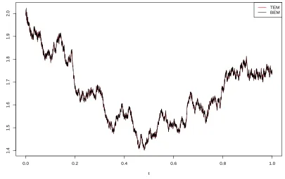
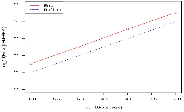
(TEM) with the backward EM (BEM). We will hence use the TEM and BEM to carry out the numerical simulations (and we choose ε = 0.5 for the TEM). Figure 5.1 shows the computer simulations of the sample paths ofx(t) by the TEM and BEM, respectively, with stepsize 10−5. We see that both sample paths are almost identical. We also perform 1000 sample paths of the TEM and BEM solutions for each of stepsizes 10−3,10−4, 10−5 and 10−6. The log-log plot of the strong errors against the stepsizes is shown in Figure 5.2. Comparing it with the dashed reference line of slop 1, we observe that the order of the strong error between the TEM and BEM is 1. But the BEM method has order 0.5 inL1-convergence so we see that our TEM also has the order 0.5 in L1-convergence. This supports our theoretical results.

0.0 0.2 0.4 0.6 0.8 1.0

1.4

1.5

1.6

1.7

1.8

1.9

2.0

t

x(t)

TEM BEM

Figure 5.1: Computer simulations of a sample path ofx(t) by the TEM and BEM with stepsize 10−5: red for TEM and black for BEM.

5

Conclusions

This is the continuation of our recent paper [23], where the truncated EM method was initiated for the multi-dimensional nonlinear SDEs. Under some additional conditions to those imposed in [23], we have discussed the Lq-convergence rates of the truncated EM method and showed that the order of Lq-convergence could be arbitrarily close to q/2. Several examples have been discussed to illustrate our theory. The computer simulations also support our theoretical results.

Acknowledgements

−6.0 −5.5 −5.0 −4.5 −4.0 −3.5 −3.0

−8

−7

−6

−5

−4

−3

log_10(stepsize) log_10(E(max|TEM−BEM|) ●

●

●

●

Error Ref line

Figure 5.2: The strong errors between TEM and BEM. The dashed reference line has slop 1.

(RKES115071), the London Mathematical Society (11219), the Edinburgh Mathematical So-ciety (RKES130172), and the Ministry of Education (MOE) of China (MS2014DHDX020) for their financial support.

References

[1] Anderson D. and Mattingly J., A weak trapezoidal method for a class of stochastic differ-ential equations. Commun. Math. Sci. 9(1) (2011), 301-318.

[2] Appleby J. A.D., Guzowska M., Kelly C. and Rodkina A.,Preserving positivity in solutions of discretised stochastic differential equations. Appl. Math. Comput. 217 (2010), 763-774.

[3] Bahar A. and Mao X., Stochastic delay population denamics. Journal of International Ap-plied Math. 11(4)(2004), 377-400.

[4] Burrage K. and Tian T., Predictor-corrector methods of Runge-Kutta type for stochastic differential equations. SIAM J. Numer. Anal. 40(4) (2002), 1516-1537.

[5] Burrage P. M. and Burrage K.,A variable stepsize implementation for stochastic differential equations. SIAM J. Sci. Comput. 24(3)(2002), 848-864.

[6] Ginzburg V. L., Landau, L. D., On the theory of superconductivity. Zh. Eksperim. i teor. Fiz. 20(1950), 1064-1082.

[7] Gy¨ongy I.,A note on Euler’s approximations. Potential Anal. 8(3) (1998), 205-216.

[8] Higham D.J. and Mao X., Convergence of Monte Carlo simulations involving the mean-reverting square root process. Journal of Computational Finance, 8(3) (2005), 35-62.

[10] Higham D.J., Mao X., Yuan, C.,Almost sure and moment exponential stability in the nu-merical simulation of stochastic differential equations. SIAM J. Numer. Anal. 45(2) (2007), 592-609.

[11] Hu Y., Semi-implicit Euler-Maruyama scheme for stiff stochastic equations. Stochastic Analysis and Related Topics, V (Silivri, 1994), 183-202, Progr. Probab., 38, Birkh¨auser Boston, Boston, MA, 1996.

[12] Hutzenthaler M. and Jentzen A.,Numerical approximations of stochastic differential equa-tions with non-globally Lipschitz continuous coefficients, arXiv:1203.5809.

[13] Hutzenthaler M., Jentzen A. and Kloeden P., Strong and weak divergence in finite time of Euler’s method for stochastic differential equations with non-globally Lipschitz continuous coefficients. Proc. R. Soc. A 467 (2011), 1563-1576.

[14] Hutzenthaler M., Jentzen A. and Kloeden P., Strong convergence of an explicit numerical method for SDEs with non-globally Lipschitz continuous coefficients. Ann. Appl. Probab. 22(2) (2012), 1611-1641.

[15] Khasminskii R.Z. , Stochastic Stability of Differential Equations, Alphen: Sijtjoff and No-ordhoff, 1980. (Translation of the Russian edition, Moscow, Nauka 1969).

[16] Jentzen A., Kloeden P. and Neuenkirch A.,Pathwise approximation of stochastic differential equations on domains: higher order convergence rates without global Lipschitz coefficients. Numer. Math. 112(1)(2009), 41-64.

[17] Klauder J.R., Petersen W.P., Numerical integration of multiplicative-noise stochastic dif-ferential equations. SIAM J. Numer. Anal. 22(1985), 1153-1166.

[18] Kloeden P. E. and Platen E., Numerical Solution of Stochastic Differential Equations, Springer-Verlog, Berlin, 1992.

[19] Lewis A.L.,Option Valuation under Stochastic Volatility: with Mathematica Code, Finance Press, 2000.

[20] Liu W. and Mao X.Strong convergence of the stopped Euler-Maruyama method for nonlinear stochastic differential equations. Applied Mathematics and Computation 223 (2013), 389– 400.

[21] Mao X.,Stochastic Differential Equations and Applications, 2nd Edition, Horwood, Chich-ester, UK, 2007.

[22] Mao X.,Numerical solutions of stochastic differential delay equations under the generalized Khasminskii-type conditions. Appl. Math. Comput. 217(2011), 5512-5524.

[23] Mao X., The truncated Euler–Maruyama method for stochastic differential equations, J. Comput. Appl. Math., in press, 2015.

[24] Mao X. and Szpruch L.,Strong convergence and stability of implicit numerical methods for stochastic differential equations with non-globally Lipschitz continuous coefficients, Journal of Computational and Applied Mathematics 238 (2013), 14–28.

[25] Marion G., Mao X. and Renshaw E.,Convergence of the Euler scheme for a class of stochas-tic differential equations. Int. Math. J. 1(2002), 9-22.

[27] Milstein G. N. and Tretyakov M. V., Stochastic Numerics for Mathematical Physics, Springer-Verlag, Berlin, 2004.

[28] Milstein G. N. and Tretyakov M. V.,Numerical integration of stochastic differential equa-tions with nonglobally Lipschitz coefficients. SIAM J. Numer. Anal. 43(2005), 1139-1154.

[29] M¨uller-Gronbach T.,The optimal uniform approximation of systems of stochastic differen-tial equations. Ann. Appl. Probab. 12(2)(2002), 664-690.

[30] Oksendal B.,Stochastic Differential Equations: an Introduction with Applications, 6th Edi-tion, Springer, Berlin, 2003.

[31] Saito Y. and Mitsui T.,T-stability of numerical scheme for stochastic differential equations. World Sci. Ser. Appl. Anal. 2(1993), 333-344.

[32] Song M., Hu L., Mao X. and Zhang L.,Khasminskii-Type theorems for stochastic functional differential equations. Discrete and Continuous Dynamical Systems B 18(6) (2013), 1697-1714.

[33] Sabanis S., A note on tamed Euler approximations. Electron. Commun. Probab. 18(47) (2013), 1-10.

[34] Szpruch L., Mao X., Higham D. and Pan J.,Numerical simulation of a strongly nonlinear Ait-Sahalia type interest rate model. BIT Numerical Mathematics 51(2011), 405–425.

[35] Tretyakov M.V. and Zhang Z.,A fundamental mean-square convergence theorem for SDEs with locally Lipschitz coefficients and its applications. SIAM Journal of Numerical Analysis 51 (2013), 3135-3162.

[36] Valinejad A. and Hosseini S. M.,A variable step-size control algorithm for the weak approx-imation of stochastic differential equations. Numer. Algorithms 55(4)(2010), 429-446.

[37] Wu F., Mao X. and Chen K., A highly sensitive mean-reverting process in finance and the Euler-Maruyama approximations. J. Math. Anal. Appl. 348(2008), 540-554.

[38] Wang X. and Gan S., The tamed Milstein method for commutative stochastic differential equations with non-globally Lipschitz continuous coefficients, J. Differ. Equ. Appl. 19(3) (2013), 466-490.