Constrained models for optical absorption tomography

A Constrained Solver for Optical Absorption

Tomography

N

P

, A

T

, E

F

, A

C

, H

M

C

,

L

D

, P

W

, M

L

, T

B

, D

W

,

G

H

,

W

J

1_{School of Engineering, Institute for Digital Communications, University of Edinburgh, Edinburgh, UK.} 2_{Department of Electronics and Informatics, Vrije University Brussels, Brussels, Belgium.}

3_{School of Electrical & Electronic Engineering, University of Manchester, Manchester, UK.} 4_{Department of Engineering, Photonics, Strathclyde University, Glasgow, UK.}

*_{Corresponding author: [email protected]}

Compiled September 25, 2017

We consider the inverse problem of concentration imaging in optical absorption tomography with lim-ited data sets. The measurement setup involves simultaneous acquisition of near infrared wavelength-modulated spectroscopic measurements from a small number of pencil beams equally distributed among six projection angles surrounding the plume. We develop an approach for image reconstruction that in-volves constraining the value of the image to the conventional concentration bounds and a projection into low-dimensional subspaces to reduce the degrees of freedom in the inverse problem. Effectively, by re-parameterising the forward model we impose simultaneously spatial smoothness and a choice between three types of inequality constraints, namely positivity, boundedness and logarithmic boundedness in a simple way that yields an unconstrained optimisation problem in a new set of surrogate parameters. Test-ing this numerical scheme with simulated and experimental phantom data indicates that the combination of affine inequality constraints and subspace projection leads to images that are qualitatively and quan-titatively superior to unconstrained regularised reconstructions. This improvement is more profound in targeting concentration profiles of small spatial variation. We present images and convergence graphs from solving these inverse problems using Gauss-Newton’s algorithm to demonstrate the performance and convergence of our method. © 2017 Optical Society of America

OCIS codes: (110.1758) Computational imaging; (110.6960) Tomography; (120.1740) Combustion diagnostics

http://dx.doi.org/10.1364/ao.XX.XXXXXX

1. INTRODUCTION

Chemical Species Tomography (CST) aims to image the con-centration of chemical species present in gas mixtures [1]. Its application to carbon dioxide (CO2) in gas turbine aero-engine exhausts is motivated by the aviation industry’s need to reduce CO2emissions and to enable the analysis of emissions data in order to diagnose engine condition [2], [3]. As CO2is a major product of the combustion process, it provides a good proxy to understand the complex phenomena that govern the perfor-mance of advanced gas turbines and predict irregularities and faults. Moreover, imaging the concentration of carbon dioxide in a jet’s exhaust plume enables the assessment of the performance of novel aviation fuels at full-scale operating conditions. CST was initially inspired by the success of X-ray computed tomog-raphy, and has since been developed into an optical imaging

in-version framework [9]. Existing algorithms are predominantly algebraic using inverse problem regularization tools, see for ex-ample the early work [10] and the more recent [11], [12], [13]. The use of statistical imaging methods is less by comparison, and some notable examples include the simulated annealing algorithm in [14] and the Bayesian estimation in [15], [8] and [12], who have developed algorithms for maximum a posteriori estimation assuming Gaussian priors and measurement likeli-hood probability density functions. As a detailed review of CST is beyond the scope of this paper, we mention that historical milestones and recent advances of the method are succinctly summarised in the recent review [16] and the book chapter [1]. To what concerns the novelty of this work we note that while spatial smoothness-imposing filters have been introduced and analysed in both the optimisation and statistical paradigms of the problem, to the best of our knowledge linear inequality con-straints have not yet been considered in CST. As we elaborate next, our proposed optimisation-based scheme, inspired from the geophysical literature [17], enforces smoothness in the tar-geted image explicitly in the form of heuristically chosen basis functions as well as inequality constraints for positivity and boundedness by reformulating the model. In effect, this yields

anunconstrained inverse problemand aconstrained modelthat is

directly amenable for a variety of alternative inverse problem formulations, e.g. sparsity promoting, total variation or levelset regularisation [18], [19]. Unfortunately, these advantages come at the cost of loosing the original model’s linearity and thus a direct analytical inverse solution is no longer feasible, while the Bayesian setting results in a non-Gaussian posterior for the surrogate parameters, which complicates the inference calcu-lations [8]. Moreover, the use of global basis functions as we advocated in [13] in reducing the dimensionality of the problem poses limitations to the statistical approaches that rely on com-puting image covariances and constructing prior densities from uncorrelated samples [15]. It should however be emphasised that whatever choice of basis is made, it is entirely heuristic, and a low-dimensional basis for the continuous concentration field with insignificant approximation error cannot be found without a priori knowledge of the targeted image. In dealing with infinite dimensional linear models, the approximation into a finite basis can be treated systematically by considering the resulting approximation error as a random variable [20].

To initiate the reader into the CST spectroscopic measure-ment models we provide a brief introduction to the fundameasure-mental relations, and fix our notation for the subsequent sections. Fol-lowing the notation in [21] and assuming the beam intensity at-tenuates exponentially to the intervening medium’s absorbance α≥0, then the ratio of irradiance flux density at the detectorId

[Wcm−2]to that at the sourceIsat a distanceL[cm]is given by Beer-Lambert’s law

Id

Is

ν

=e−α(ν)_{, (1)}

then the spectral absorbance is

α(ν) =

Z

Ldl kν(x), (2)

wherekν[cm−1]is the spectral absorption over the wavenumber perturbationν→ν+δνandxis the spatial coordinate. If the light is measured at wavenumberν[cm−1]andxdenotes the spatial coordinate then

kν(x) =Sν(x;T)φν(x;T,P,X)Ps(x), (3)

whereSν(x;T) [cm−2atm−1]is the temperature-dependent

line-strength andφν(x;T,P,X) [cm]is the line-shape function atν

that depends both on the temperature and pressure of the gas

andPs(x) [atm]is the partial pressure of thesth species, in this

case the CO2. To compute the spectral measurement we dis-cretise the profiles of temperature, total gas pressure and mole fraction in a 2D spatial basis of functions defined on the optical plane to obtainT(x) [K],P(x) [atm]and the molar fraction func-tionX(x)respectively, sincePs(x) =P(x)X(x). Importing data from the HITRAN database [22] at wavenumbers{ν1, . . . ,νN} in the vicinity of the measured frequencyνwe can model the spectral absorbance of the species by approximating the profiles ofSνandφνat the resolution of the above bases using the

def-initions in [21]. In effect the spectroscopic measurement atν becomes

α(ν)=. log Is

Id

νj

≈

N

∑

Z

Ldl Sνj

(x;T)φνj(x,ν;T,P,X)P(x)X(x),

(4)

while the approximation sign indicates that the relation is semi-empirical and depends on the availability and accuracy of the HITRAN data. Given measurements atMdistinct wavenumbers

{α(ν1), . . . ,α(νM)} when the temperature and total pressure profiles along the beam trajectory are known then Eq. (4) can be reduced to a weighted line integral for the sought concentration (mole fraction) function

α(νi) =

Z

Ldl N

∑

ζj(x,νi)X(x), i=1, . . . ,M, (5)

whereζj(x,νi) =Sνj(x)φνj(x,νi)P(x)is a known weight

func-tion. Note that even whenPandTare uniform, theζjfunctions are not, thus Eq. (5) requires some model fitting techniques in order to extract the so-called ‘path concentration data’ along the beam when knowing the{ζ1, . . . ,ζN}and{α(ν1), . . . ,α(νM)} [16].

2. A LINEAR ATTENUATION MODEL FOR CONCENTRA-TION

We consider the inverse problem in CST for reconstructing the concentration imageχbased on the measurement model Eq. (4) at a single wavenumber. Following the Radon trans-form paradigm [9], in a finite dimensional setting the integral equation leads to a discrete linear attenuation model

y=Aχ+e, (6)

whereA∈Rm×n_{is the discretised measurement operator,} χ∈

Rn _{is the discrete concentration parameter that is piecewise} constant on the support of the model elements andeis additive zero-mean noise. Based on Eq. (5) the measurement at theith beam of the system is defined as

yi=.

Z

Li

dl X(x), i=1, . . . ,m. (7)

We are interested in the situations where the degrees of freedom

solutions, making the reconstruction of the concentration prob-lematic. More precisely, ifm<nthenAhasmclosely clustered singular values and, theoretically speaking,n−mzero singular values. While its smallest non-singular value can be shown to be well above zero, see section 9.5 in [9] for the analytical definition of the singular values of the Radon transform and [13] for a numerical justification, the matrix is rank-deficient. To rectify the situation one typically applies some form of regularisation, usually of a Tikhonov-type [23], that stabilises the inversion and yields imaging with adequate stability and resolution. When the number of image parameters, e.g. voxels,nis large, Tikhonov (c.f. Eq. (24)) becomes computationally expensive, and challeng-ing to optimise.

Our approach seeks to enforce some affine inequality con-straints to bound the concentration to its admissible range[0, 1], and to reduce the dimension of the default ‘pixel-based’ parame-ter space by projecting its image onto a subspace of global basis functions that are consistent with its expected smooth features. The methodology we propose has two distinct phases: We first model the concentration using a family of surrogate functions and then formulate the inverse problem with respect to a new set of parameters projected onto a low-dimensional subspace. This approach provides a straightforward way to transform the inverse problem into a low-dimensional unconstrained optimi-sation problem for a differentiable cost function. Its appeal lies primarily in the embedding of the inequality constraints into the model as oppose to constraining the inverse problem, its simplicity of implementation, and its computational robustness as it requires very little tuning. Although other alternatives exist within the framework of constrained optimisation algorithms, such as the projected gradients [24], active sets [25], linear pro-gramming and interior point methods [18], these algorithms are more complex and computationally expensive by comparison.

We describe our methodology by extending our previous work in [13], beginning with some important definitions. The subspace of bounded vectors inS1⊂Rn

S1=. {χ∈Rn|`≤χ≤u}, where 0< ` <u, (8) for some finite bounds`andu. Further let a continuous and invertible, one-to-one mappingυ:Rn→ S1. Then there exists a unique vector of unconstrained parametersρ∈Rnsuch that

χ=υ(ρ), ∀x∈ S1. (9)

We aim to compute the projection of the high-dimensionalρin a low-dimensional space of basis functionsS₂⊂Rn_{, such that}

S₂=. {Qr|r∈Rs_{}, (10)} whereQ∈Rn×s_{is a matrix whose columns form an} orthonor-mal basis of some feature functions{φ1, . . . ,φs}withs n. This arrangement allows to formulate an inverse problem for the projection of the unconstrained vector of parametersρinS2, from which we ultimately obtain a constrained concentration image

ˆ

χ=υ(Πρˆ), where Πρ=Qρ, (11)

forΠ:Rn→ S2the associated projection matrix operator. This framework enforces affine inequality constraints on the admissi-ble range of the image while it approximates the solution within a subspace of basis functions that are consistent with the ex-pected features of the concentration image. For the targeted CST application the benefit of this approach is twofold: It constrains the concentration image within its intrinsic [0,1] bounds, and

thereafter it allows to formulate the inverse problem for the log-arithm of the concentration and thus making it more suitable to image multiscale concentration functions [17]. In the next section we present the foundation of our approach, namely the use of nonlinear surrogate functions that are suitable to model the constraints on the concentration image.

3. SURROGATE FUNCTIONS

For a fixedS₁, we can find a re-parameterisation ofχ∈ S1via an invertible and analytic mapping

υ:R→ S1 (12)

that we name the surrogate mapping. The invertibility provides υwith the simultaneous surjectivity and injectivity, whereas the analyticity providesυwith infinite differentiability. The most simple and practical manner to insure invertibility consists in considering mappings that are strictly monotonic.

We describe a practical method that can be used to obtain a surrogate mapping, by extending and generalising the pricee-dure in [17]. We focus initially on a surrogate mapping that satisfies the strict positiveness of the concentration. Thereafter, we show how we can reuse this surrogate mapping in order to obtain another surrogate mapping that boundsχor its logarithm between two strictly positive bounds.

A. Strict positiveness.

IfS1is the set of the real numbers that are larger than a real number` >0 then the following invertible and analytic function

υp(ρ;`)=. eρ+`, ∀ρ∈R,

is a model of the surrogate mapping Eq. (12). In particular, υp(ρ; 0)is the inverse of the logarithmic function that has already been proposed as a model of the inverse mapping of Eq. (12) [17].

B. Boundedness.

Consider the following function

υs(ρ;`,u)=. `+ u−` 1+ρ−1,

∀ρ∈R, ∀`,u∈R, ` <u.

IfS1is the set of the real numbers in the open interval of end-points`andu, with 0< `, then for a real numberqsuch that 0≤q≤uwe can define the following invertible and analytic function

υb(ρ;`,q,u)=. υs(υp(ρ;`−q);`,u) =`+ u−` 1+ (eρ<sub>+`−q)</sub>−1,

(13) ∀ρ∈R, so that

υb(ρ;`,`,u) =`+ u−`

1+e−ρ, ∀ρ∈R, is just another expression of a model of Eq. (12).

C. Logarithmic boundedness.

A particular case of boundedness occurs when we considerχin an interval that is spanning over several orders of magnitude, or when the interval is extremely narrow. In such cases, it is more appropriate to bound the logarithm ofχ. Indeed by noting that

then by using a function

υl(ρ)=. logρ, ∀ρ∈R, s.t.ρ>0,

and the mappingυpdescribed inA, we can relate the bounded-ness of logχto the ordinary boundedness described inB. For ρ=logχit follows thatρ=υl(υp(ρ; 0))and thus

υl◦υp: logχ7→υb(ρ;`,`,u).

Note that ifS₁is the set of the real numbers that are strictly positive and whose logarithm is in the open interval with end-points`andu, thenυb(ρ;`,`,u)is not a model of the surrogate mapping Eq. (12), becauseυbmapsρ∈ Rto logχinstead of χ. However, since the range ofυb(ρ;`,`,u)is the interval with endpoints`andu, sinceχcan be obtained fromυbunivocally, then

υp(υb(ρ;`,`,u); 0)

always mapsχontoS1, and it is just another expression of a model of Eq. (12).

D. Generic surrogate mapping.

According to the constraints applied onχ, using the invertible and analytic mappings described inA-C, we can define a model of the surrogate mapping Eq. (12) as follows:

υ(ρ)=.



 

 

υp(ρ;`) ifS1={0< ` <χ} (14a) υb(ρ;`,`,u) ifS1={0< ` <χ<u}(14b) υp(υb(ρ;`,`,u); 0) ifS1={` <logχ<u} (14c)

Notice that Eq. (14a) is a special case of Eq. (14b). Indeed, if in Eq. (13) we replaceυswith the identity mapping id(υp) =υp thenυb(ρ;`, 0,u) = υp(ρ;`). Similarly, Eq. (14b) is a special case of Eq. (14c). Indeed, if 0 < `and we replace logχand υprespectively withxand the identity mapping id(υb) = υb thenυp(υb(ρ;`,`,u); 0) =υb(ρ;`,`,u). For this reason, we can obtain the derivatives ofυby considering only the derivatives of Eq. (14c). To keep the notation as general as possible, for all χ∈ S1andρ∈Rnwe have

χ=Υ(ρ) = [Υj(ρ)]n_j=1, Υj(ρ)=. υ(ρj), (15)

and we notice that ifn =1 thenΥreduces toυ. The Jacobian matrix ofΥis then shown to be

JΥ(ρ) =D

"

d dρj

υ(ρj)

#n

j=1

, (16)

where D is an operator that transforms a vectorρin the diagonal matrix whose main diagonal equalsρ. By applying the chain rule of differentiation on Eq. (14c) we obtain that

d dρj

υ(ρj) = d dυb

υp(υb(ρj;`,`,u); 0)

· d

dυpυs(υp(ρj; 0);`,u) d dρj

υp(ρj; 0)

= υp(υb(ρj;`,`,u); 0)(u−`)υp(ρj; 0)

(1+υp(ρj; 0))2

,

therefore in general the derivative ofυis

d dρj

υ(ρj) =



   

   

υp(ρj; 0) if Eq. (14a)

(u−`)υp(ρj;0)

(1+υp(ρj;0))2 if Eq. (14b) υ(ρj) (u−`)υp(ρj;0)

(1+υp(ρj;0))2 if Eq. (14c)

. (17)

4. THE PROJECTED INVERSE PROBLEM

In a previous work we have devised an approach that involved reducing the dimensionality of the sought image by projecting it into a smooth basis of orthogonal functions and thereafter regularising the projected problem [13]. We now attempt to ex-tend this framework by introducing affine inequality constraints on the values of the image. Having defined the surrogate func-tions for the concentration image we set out to cast the inverse problem with respect to the surrogate parametersρ. To stabilise the inversion we reduce the degrees of freedom in the resulting inverse problem, by adopting the following assumption. If we consider a projectionΠρ ∈ S2then we seek to reconstructχ when its corresponding surrogate imageρ=υ−1(χ)satisfies

kρ−Πρk

kρk

<1,

since ultimately our approach is restricted to reconstructing only theΠρofx. The choice of basis functionsQinvolved in the projectionΠ=Q(QTQ)−1QTis made to impart some level of smoothness to the expected image, as this is consistent with the expected profile of the concentration and plume velocity. From the surrogate form of model Eq. (6),

y=Aυ(ρ) +e, (18)

linearising at pointρ(i)yields

y≈A υ(ρ(i)) +JΥ(ρ(i))(ρ−ρ(i))+e, (19)

and thus imposingΠρ=Qrand setting

y(ρ(i)) =y−Aυ(ρ(i)) +AJΥ(ρ(i))ρ(i), K(ρ(i)) =AJΥ(ρ(i)),

we arrive at theith projected surrogate model

y(ρ(i)) =K(ρ(i))Qr+e˜, (20)

with the noise ˜enow including also the projection approxima-tion error. In the context of the Gauss-Newton algorithm, an image can be reconstructed iteratively by solving the regularised problems

ˆ

r(i+1)=argmin r∈_Rs

n

y(ρ(i))−K(ρ(i))Qr

2

+λ2r−r(i)k2

o

,

(21) fori=1, 2, . . . whereλis a regularisation parameter,Πρ(i) =

Qr(i)_{, and JΥthe Jacobian of}

can be efficiently traced based on a heuristic criterion originally proposed in [13]. Ultimately, the reconstructed concentration image can be obtained from Eq. (21) by

ˆ

χ(i)=υ(Qrˆ(i)). (22)

For the sake of comparison, we also compute the constrained linear least squares inverse problem for the original parameters

ˆ

χc=argmin

χ∈_Rn

n

_A

λR

χ−

_y

λRχ0

2o

, for

(

χ>0

`≤χ≤u (23) using an active sets algorithm as this is implemented in Mat-lab’s functionslsqnonnegandlsqlinfor the nonnegative and box constrained cases respectively [28]. The unconstrained in-stance of Eq. (23) constitutes to solving the generalized Tikhonov problem

ˆ

χt = (ATA+λ2RTR)−1(ATy+λ2RTRχ0), (24)

for an initial guesstimateχ0. The comparison with Tikhonov solutions is appropriate for a number of reasons. Tikhonov reg-ularisation is among the most popular regreg-ularisation strategies in inverse problems and CST in particular. Moreover, its an-alytic formulation allows for a direct application to a default constrained optimisation solver, such as those included in Mat-lab, from where we compute images for comparison. Thirdly, the Tikhonov problem bares an evocative resemblance to the maximum a posteriori estimator in the Bayesian inverse prob-lem, subject to a suitably smooth prior density [8], [15], and lastly upon the appropriate choice of the regularization matrix and parameter it can impose the required smoothness in the un-known image profile, which makes is compatible to our method. Note however that our scheme enforces smoothness explicitly by selecting a (particular) basis for the projection in Eq. (11), while Tikhonov imposes smoothness indirectly by correlating the values of the image according to their distance.

5. NUMERICAL RESULTS

In this section we present some results obtained from numerical simulation experiments. Data were computed from Eq. (6) based a high resolution grid withn=10000 elements for a target con-centration imageχand then infused with zero-mean Gaussian noise at a standard deviation of 10% of each data value. The model was constructed to simulate the measurements of the FLITES system [3] based on a beam arrangement of six projec-tion angles at{0, 30, 60, 90, 120, 150}degrees, each comprising twenty one parallel beams, as shown in the schematic of figure1. To investigate the performance of our methods in reconstructing concentration profiles with low and high spatial variation we consider two distinct tests with targetsχ∗_l andχ∗_h, as sums of Gaussian functions

χ∗(x) =

5

∑

χi(x), χi(x) =|χi|exp

n−(x−x0

i)2 2σ_i2

o

, (25)

where the specific amplitudes|χ|, centresx0and spreadsσare tabulated in table1.

To assess the quality of the reconstructed images ˆχand the convergence of the algorithm we compute the standard relative errors for the data and images, which from Eq. (22) are given by

ηD(χˆ)=.

ky−Aχˆk

kyk , and ηI(χˆ)

.

=kχˆ−Πχ

∗_k

kΠχ∗k , (26)

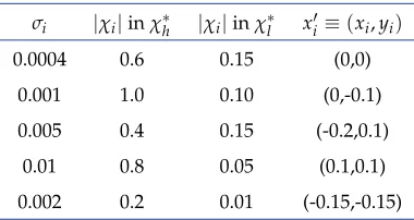
Table 1.Specifications of the synthetic high-variation and

low-variation concentration profileχ∗_handχ∗_l respectively in Eq. (25).

σi |χi|inχ∗_h |χi|inχ∗_l x0_i≡(xi,yi)

0.0004 0.6 0.15 (0,0)

0.001 1.0 0.10 (0,-0.1)

0.005 0.4 0.15 (-0.2,0.1)

0.01 0.8 0.05 (0.1,0.1)

0.002 0.2 0.01 (-0.15,-0.15)

Fig. 1. A schematic of the physical FLITES ring with the 126

recalling that as we showed in [13], due to the subspace projec-tion induced informaprojec-tion loss the ‘best’ image we can hope to recover for a targetχ∗isΠχ∗.

The high variation concentration target is bounded by 3×

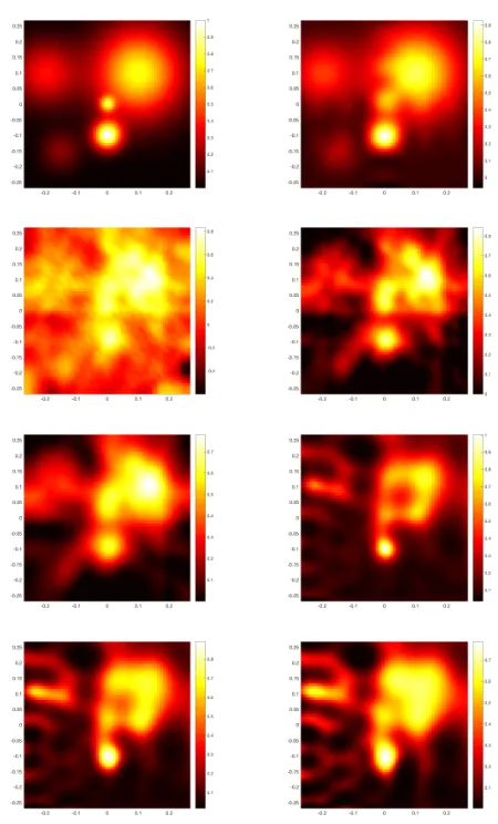
10−4 ≤ χ∗_h ≤ 1 and for this test we have used a subspace of 225 radial basis functions, orthonormalized through the Gram-Schmidt process [28]. In turn this led to a projection approxi-mation error ofkρ∗_h−Πρ_h∗k/kρ∗_hk ≈0.12 which sets the lower bound of the image reconstruction error. We run the algorithm for the three types of surrogate mappings and compare the results with that obtained from the unconstrained and con-strained forms of the Tikhonov solution in Eq. (24) and Eq. (23) respectively, for a smoothness imposing regularisation matrix

R ∈ Rn×n_{based on the definition in [1] and a uniform prior} guessχ0. For the inverse problem the model Eq. (6) was discre-tised on a courser grid comprisingn =3600 voxels on which we have also approximated the target and its projection to aid the visual assessment of the reconstructions and the evaluation of the error measures in Eq. (26). The images in figure2, show that the performance of our scheme is superior to that of the unconstrained Tikhonov method, which yields irrational nega-tive concentration values and is comparable to the constrained Tikhonov solutions. The images of the proposed method corre-spond to running 5 Gauss-Newton iterations on the projected inverse problem for the surrogate parameters with a value of λaround 10−2. In this ‘high-variation’ benchmark the three surrogate formulations perform equally well, converging almost simultaneously after the first 5 iterations as shown in the left column of figure4. The unconstrained Tikhonov solution with the same data and a manually adjustedλ=1 attains a smaller relative data error atηD =2.2×10−4but the relative error in the image is much higher atηI =0.37. To minimise bias in the comparison all initial prior guess images were chosen to be posi-tive and homogenous. The nonnegaposi-tive and bounded Tikhonov solutions were computed based on the Matlab commands af-ter 3400 and 1893 iaf-terations respectively to relative data errors 0.013 and 0.042, and image errors at 0.244 and 0.217. It is also worthwhile mentioning that for the coarse grid with 3600 param-eters, executinglsqnonnegandlsqlinon a 3.4 GHz Intel Core i7 Mac with 32GB RAM took about 16 and 11 minutes respec-tively while the 5 iterations of our algorithm took on average for all three surrogates about 5 seconds. Indicatively, we note that the assembling and othogonalization of the projection bases matrixQtook about 4 seconds while the switching between original and surrogate parameters as in Eq. (22) required less than a second.

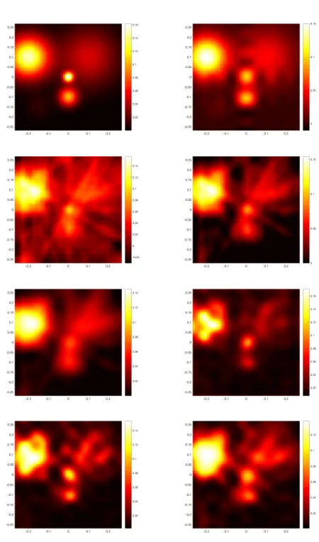
To investigate the utility of our method in reconstructing concentration profiles of low variation we perform a simi-lar simulation on a targetχ∗_l whose values are in the range 1.5×10−5 _{≤ χ}∗

l ≤0.16 as shown in3. Keeping the signal to noise ratio fixed, we compute regularisation values and con-trol the number of iterations using the discrepancy principle after 5 iterations we arrive at the images illustrated in figure

3and the convergence plots forηDandηI on the right hand column of figure4. Similar to the ‘high-variation’ case results our methodology seems to perform better than unconstrained Tikhonov regularisation whereηI=0.30 andηD=1.15×10−4, despite that the subspace projection error is larger, see for ex-ample the images in the top row of figure3. This set of results reveals also that in this case bounding the values of the image or indeed the logarithm of the image improves the reconstruction, both in terms of the spatial resolution of the images but also in

Fig. 2.At the top row the high-variation target imageχ∗_hin

terms of the convergence of the reconstruction algorithm. The graphs at the right column of figure4show that the bounded and logarithmically bounded iterations converge faster than the positivity case, while the graph of the relative image error shows again the issue of divergence in the solution after the first 6 or so iterations highlighting the need for a stoping crite-rion. In terms of the image errors, those of our algorithm are very similar, if not marginally better, to those of the constrained solvers in Matlab atηI =0.18 andηI =0.20 for the positive and box bounded solutions compared toηI =0.24 andηI = 0.23 obtained bylsqnonnegandlinlsqrespectively. In terms of the relative data errors, the unconstrained Tikhonov was again the lowest atηD =1.15×10−4while those of the constrained version were similar to those obtained for our algorithm (c.f. figure4) atηD = 0.027 andηD = 0.064 for the nonnegative and bounded cases. In terms of the computational complexity, the Matlab solvers take in excess of 10 minutes each for 3030 iterations forlsqnonnegand 5388 iterations inlinlsq.

A. Tuning the regularisation parameter

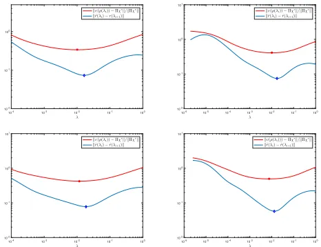
In [13] we have proposed a heuristic method for choosing the regularisation parameter for the linear projected inverse prob-lem, without any surrogate variable transformation. According to this we compute the linearised solution Eq. (21) on a sequence of logarithmically equidistant values ofλ, ranging from the largest singular value ofKQto its smallest non-zero singular value. We then compute the norm of the difference between every two successive solutions and plot them against the mid-point average values of the regularisation parameter. As we argued in [13], given the rank deficiency of the projected, and now surrogate projected model we expect the optimal value of λnear the minimum of the graph within that range ofλvalues

∆r(ˆ λj) =kr(ˆ λi)−r(ˆ λi+1)k, λj=

1

2(λi+λi+1). (27)

To verify and demonstrate this criterion we compute the so-lutions at 500 regularisation parameters and plot the running difference norm∆rˆagainstλin figure5, along with the norm of the discrepancy between eachλ-dependent solutions to the true projected solutionΠχ∗. The graphs, which refer to the bounded and logarithmically bounded surrogate problems for the two test casesχ∗_handχ∗_l show that the two curves attain a minimum around the same value ofλ, e.g. close to 10−2. To aid stability the model Eq. (6) is scaled so thatkAk = 1, and sinceQhas orthonormal columns the maximum singular value ofKQ = AJΥQis around 1. The time required to solve these problems for eachλwas about 1 minute, since despite having to solve 500 different instances, the systems were low-dimensional.

6. REAL DATA RECONSTRUCTION

At the FLITES experiment an optical imaging ring has been con-structed [3] to provide 126 simultaneous measurements of CO2 equally arranged in 6 projection angles, using the calibration-free 2f/1f wavelength modulation spectroscopy technique (TDLS-WM) [5]. The light sources and sensors are positioned perimet-rically at a 12-sided ring of 7 m in diameter. In this section we present some reconstructions from measurements obtained from controlled phantom experiments using this system. The data correspond to two circular, almost homogenous carbon dioxide plumes arranged diagonally with respect to the centre of the computational domain, one at 40 cm diameter and the other at

Fig. 3.At the top row the low-variation target imageχ∗_l in a

0 5 10 15 20 25 Iteration index 10-2 10-1 100 101 R el at iv e d at a er ror Positivity Boundedness Log boundedness

0 5 10 15 20 25

Iteration index 10-2 10-1 100 101 102 R el at iv e d at a er ror Positivity Boundedness Log boundedness

0 5 10 15 20 25

Iteration index 100 R el at iv e im age er ror Positivity Boundedness Log boundedness

0 5 10 15 20 25

Iteration index 10-1 100 101 102 R el at iv e im age er ror Positivity Boundedness Log boundedness

Fig. 4.At the top the relative data errorηD(χˆ)reduction plots

at each Gauss-Newton iteration for the three surrogate trans-formations during theχ∗_h(left) andχ∗_l (right) tests. Below the corresponding curves for the image errorsηI(χˆ)for the same tests and surrogates. The graphs demonstrate the requirement for terminating the iterations in order to avoid fitting the noise into the images, i.e. note the divergence in the bottom row af-ter iaf-teration 6, while the data errors in the upper row continue to reduce. Comparing between the two tests, the graphs to the left show that convergence and error reduction is similar for all three choices of surrogates, while those to the right for χ∗_l show that the boundedness and logarithmic boundedness iterations converge much faster than the positivity case. The errors are computed based on the formulas Eq. (26).

10-4 10-3 10-2 10-1 100

λ

10-2

10-1

100

kυ(ρ(λi))−Πχ∗k/kΠχ∗k kˆr(λi)−r(λi+1)k

10-6 10-5 10-4 10-3 10-2 10-1 100

λ

10-2

10-1

100

101

kυ(ρ(λi))−Πχ∗k/kΠχ∗k kˆr(λi)−ˆr(λi+1)k

10-4 10-3 10-2 10-1 100

λ

10-2

10-1

100

101

kυ(ρ(λi))−Πχ∗k/kΠχ∗k kˆr(λi)−ˆr(λi+1)k

10-6 10-5 10-4 10-3 10-2 10-1 100

λ

10-2

10-1

100

101

kυ(ρ(λi)))−Πχ∗k/kΠχ∗k kˆr(λi)−ˆr(λi+1)k

Fig. 5. Choosing the regularisation parameters. The range of

values forλbeginning at the smallest singular value ofKQ before the rank deficiency jump in the spectrum and ending its largest singular value that was normalised to be 1. The star marker on the red curve denotes the optimal value ofλ while the diamond is the computed minimum of the curve in Eq. (27). Note that normally only the blue curve can be com-puted, and the red curve is plotted here merely for validation.

−0.2 −0.1 0 0.1 0.2 −0.25 −0.2 −0.15 −0.1 −0.05 0 0.05 0.1 0.15 0.2 0.25 −0.03 −0.02 −0.01 0 0.01 0.02 0.03 0.04 0.05

−0.2 −0.1 0 0.1 0.2 −0.25 −0.2 −0.15 −0.1 −0.05 0 0.05 0.1 0.15 0.2 0.25 0.01 0.02 0.03 0.04 0.05 0.06 0.07

−0.2 −0.1 0 0.1 0.2 −0.25 −0.2 −0.15 −0.1 −0.05 0 0.05 0.1 0.15 0.2 0.25 0.01 0.02 0.03 0.04 0.05 0.06 0.07 0.08

−0.2 −0.1 0 0.1 0.2 −0.25 −0.2 −0.15 −0.1 −0.05 0 0.05 0.1 0.15 0.2 0.25 0.01 0.02 0.03 0.04 0.05 0.06 0.07 0.08

Fig. 6. At the top row the high-dimensional Tikhonov

solu-tion and the image reconstrucsolu-tion with the positiveness surro-gate. Below the corresponding images with boundedness and logarithmic boundedness constraints.

60 cm. The concentration of the gas was measured to be approx-imately 6% for both plumes, using a flue gas analyser (Kane 455). The optical signal was generated using a master oscillator power amplifier configuration. The seed laser was an Eblana Photonics Multi Quantum Well Distributed Feedback (DFB) laser (EP1997-DMB01-FM), whose output power could be amplified to a maximum of 2 W using a Thulim Doped Fibre Amplifier designed and manufactured by the University of Southampton [27]. The output from the amplifier is distributed around the hosting ring using a bespoke optical fibre network, providing 126 optical beams to be directed through the imaging space. The seed laser current was modulated at 5 Hz and 100 kHz for the purpose of using the 2f/1f calibration-free tunable diode laser spectroscopy with wavelength modulation technique [5]. The individual photo-diode outputs from the 126 channels were recorded using an NI-PXI-6366 data acquisition (DAQ) board at 2MS/s. As the DAQ only allows 8 channels to be recorded simultaneously an NI-PXI 2530B multiplexor was used to con-secutively switch between the 126 channels, giving a full data acquisition rate of about 0.3 Hz. The recorded signals were demodulated using a bespoke LabVIEW based lock-in ampli-fier and the path-integrated mole-fraction measurements were obtained using the methodology described in [16].

In the image reconstruction we have used the same surro-gate formulations as in the simulated cases, although in this case we have projected the surrogate problem into a basis of 64 discrete cosine basis functions. The resulted images after 4 Gauss-Newton iterations are presented in figure6, for the three different surrogate formulations at a relative data error of

aroundηD = 0.6. Compared to the smooth Tikhonov image,

the iterative results appear to be quantitatively and qualitatively superior. Due to the significant levels of noise in the data the dis-tinction in the diameter of the two plumes is not very profound in these images.

7. CONCLUSIONS

inequal-ity constraints. The key aspect of our approach is the use of surrogate functions that introduce these constraints within the forward model by re-parameterisation leading into an uncon-strained inverse problem formulation. This conuncon-strained model is then projected into a low-dimensional subspace to improve the stability of the inversion when having limited tomographic data. The resulting problem was then addressed using the Gauss-Newton algorithm and results from simulated and real measure-ments demonstrated that the spatial resolution of the images is significantly enhanced compared to unconstrained, Tikhonov solutions with smoothness imposing regularisation. Compared to solving the unprojected inverse problem with non-negativity and bound constraints using constrained optimisation software our method yields images of comparable quality at a small frac-tion of the time. Our computafrac-tional results indicate also that bounding the image’s value or its logarithm from above and below offers faster convergence and better accuracy in concen-tration functions with low spatial variation, although a stopping criterion is needed in order to terminate the iterations before the solution diverges. Compared to unconstrained regularised solvers the advantage of our method is both quantitative and qualitative as the concentration levels are recovered with better accuracy while at the same time the features of the images are enhanced avoiding to a large degree unwanted blurring effects.

8. FUNDING INFORMATION

We acknowledge EPSRC for funding this work in the context of FLITES : ‘Fibre-Laser Imaging of gas Turbine Exhaust Species’ project. (EP/J002151/1)

9. ACKNOWLEDGMENTS

We are grateful to Victor Archilla and coworkers at INTA Madrid for facilitating the phantom tests, and Mark Johnson of Rolls Royce for helpful discussions on jet engine combustion and emissions.

REFERENCES

1. McCann H, Wright P and Daun K 2015,Industrial Tomography: Systems and Applications, Elsevier.

2. Ma L, Li X, Sanders S T, Caswell A W, Roy S, Plemmons D H, and Gord J R, 2013,50-kHz-rate 2D imaging of tepmerature and H20 concentration at the exhaust plane of a J85 engine using hyperspectral tomography, Optics Express,21(1), 1152-1162.

3. Wright P, Mccormick D, Kliment J, Ozanyan K, Tsekenis S, Fisher E, McCann H, Archilla V, Gonzalez-Nunez A, Johnson M, Black J, Lengden M, Wilson D, Johnstone W, Feng Y, and Nilsson J, 2016,Implementation of non-intrusive jet exhaust species distribution measurements within a test facility, IEEE Aerospace Conference.

4. Twynstra M J and Daun K J, 2013,Laser-absorption tomography beam arrangement optimisation using resolution matrices, Applied Optics,51, 7059-7068.

5. Rieker G B, Jeffries J B, and Hanson R K, 2009, Calibration-free wavelength-modulation spectroscopy for measurements of gas tempera-ture and concentration in harsh environmentsApplied Optics,48(29), 5546-5560

6. Ma L and Cai W, 2008,Numerical investigation of hyperspectral tomog-raphy for simultaneous temperature and concentration imaging, Applied Optics47(21), 3751-3759.

7. Cai W and Kaminski F C, 2014,A tomographic technique for the simulta-neous imaging of temperature, chemical species, and pressure in reactive flows using absorption spectrocsopy with frequency-agile lasers, Applied Physics Letters,104.

8. Grauer S J, Tsang R W and Daun K J, 2017,Broadband chemical species tomography: Measurement theory and a proof-of-concept emission detection experiment, J. of Quant. Spectrosc. Radiat. Transf.,198, 145-154. 9. Bertero M and Boccacci P, 2002,Introduction to inverse problems in

imaging, Institute of Physics.

10. Torniainen E D, Hinz A K and Gouldin C F, 1998,Tomographic analysis of unsteady, reactive flows: numerical investigation, AIAA Journal,36(7), 1270-1278.

11. Terzija N and McCann H, 2010,Wavelet-based image reconstruction for hard-field tomography with severely limited data, IEEE Sensors Journal,

11(9), 1885-1893.

12. Daun K J 2010, Infrared species limited data tomography through Tikhonov reconstructionJ. Quant. Spectrosc. Radiat. Transf.111, 105-115.

13. Polydorides N, Tsekenis A, McCann H, Archilla V-P and Wright P 2016,

An efficient approach for limited-data chemical species tomography and its error bounds, R. Soc. A472, 2187.

14. Cai W and Kaminski F C, 2014,Multiplexed absorption tomography with calibration-free wavelength modulation spectroscopy,104

15. Grauer S J, Hadwin P J and Daun K J, 2016,Bayesian approach to the design of chemical species tomography experiments, Applied Optics,

55(21), 5772-5782.

16. Cai W, and Kaminski F C, 2017,Tomographic absorption spectroscopy for the study of gas dynamics and reactive flows, Progress in Energy and Combustion Science,59.

17. Commer M and Newman A G 2008,New advances in three-dimensional controlled-source electromagnetic inversion, Geophys. J. Int.172, 513-535.

18. Boyd S and Vandenberghe L 2004, Convex optimisation,Cambridge University Press.

19. Twynstra M G, Daun K J and Waslander S L, 2014, Line-of-sight-attenuation chemical species tomography through the level set method, J. Quant. Spectrosc. Radiat. Transf.,143, 25-34.

20. Kaipio J and Somersalo E, 2007,Statistical inverse crimes: Discreti-sation, model reduction and inverse crimes, Computational and Applied Mathematics,198(2), 493-504.

21. Hanson R K, Spearrin R M, Goldenstein C S, 2016,Spectroscopy and optical diagnostics for gases, Springer.

22. High Resolution Transmission database, www.hitran.org

23. Hansen P C, 2002,Rank-deficient and discrete ill-posed problems: Nu-merical aspects of linear inversion, SIAM.

24. Bertsekas D P 1982,Projected Newton methods for optimisation prob-lems with simple constraints, SIAM J. Contr. Opt.20(2), 221-246. 25. Gill P E, Murray W, and Wright M H 1981, Practical Optimization,

Academic Press, London, UK.

26. Hanke M 1997,A regularizing Levenberg - Marquardt scheme, with applications to inverse groundwater filtration problems, Inverse problems

13(1), 79-95.

27. Feng Y, Nilsson J, Jain S, May-Smith T C, Sahu J K, Jia F, Wilson D, Lengden M and Johnstone W, 2014,LD-seeded thulium-doped fibre amplifier for CO2measurements at 2µm, 6th Europhoton Conference (EPS-QEOD).