City, University of London Institutional Repository
Citation
:
Allefeld, C. ORCID: 0000-0002-1037-2735 and Haynes, J-D. (2013). Searchlight-based multi-voxel pattern analysis of fMRI by cross-validated MANOVA. Neuroimage, 89, pp. 345-357. doi: 10.1016/j.neuroimage.2013.11.043This is the accepted version of the paper.
This version of the publication may differ from the final published
version.
Permanent repository link:
http://openaccess.city.ac.uk/id/eprint/22834/Link to published version
:
http://dx.doi.org/10.1016/j.neuroimage.2013.11.043Copyright and reuse:
City Research Online aims to make research
outputs of City, University of London available to a wider audience.
Copyright and Moral Rights remain with the author(s) and/or copyright
holders. URLs from City Research Online may be freely distributed and
linked to.
City Research Online: http://openaccess.city.ac.uk/ [email protected]
Searchlight-based
multi-voxel pattern analysis of fMRI
by cross-validated MANOVA
Carsten Allefeldˆ1,2*ˆ; John-Dylan Haynesˆ1–6**ˆ
Affiliations:
1. Bernstein Center for Computational Neuroscience, Charit´e – Universit¨atsmedizin Berlin, Germany 2. Berlin Center of Advanced Neuroimaging, Charit´e – Universit¨atsmedizin Berlin, Germany 3. Department of Neurology, Charit´e – Universit¨atsmedizin Berlin, Germany
4. Berlin School of Mind and Brain, Humboldt-Universit¨at zu Berlin, Germany 5. Excellence Cluster NeuroCure, Charit´e – Universit¨atsmedizin Berlin, Germany 6. Department of Psychology, Humboldt-Universit¨at zu Berlin, Germany
Address for all affiliations: Charit´e-Campus Mitte Philippstr. 13, Haus 6 10115 Berlin, Germany
* E-mail: [email protected] ** E-mail: [email protected]
Corresponding author: Carsten Allefeld, Tel. +49 30 2093 6766
Preprint, published asNeuroImage, 89:345–357, 2014. doi:10.1016/j.neuroimage.2013.11.043
Abstract: Multi-voxel pattern analysis (MVPA) is a fruitful and increasingly popular complement to traditional univariate meth-ods of analyzing neuroimaging data. We propose to replace the standard ‘decoding’ approach to searchlight-based MVPA, measur-ing the performance of a classifier by its accuracy, with a method based on the multivariate form of the general linear model. Fol-lowing the well-established methodology of multivariate analysis of variance (MANOVA), we define a measure that directly charac-terizes the structure of multi-voxel data, the pattern distinctnessD. Our measure is related to standard multivariate statistics, but we apply cross-validation to obtain an unbiased estimate of its popu-lation value, independent of the amount of data or its partitioning into ‘training’ and ‘test’ sets. The estimate ˆD can therefore serve not only as a test statistic, but as an interpretable measure of mul-tivariate effect size. The pattern distinctness generalizes the Maha-lanobis distance to an arbitrary number of classes, but also the case
where there are no classes of trials because the design is described by parametric regressors. It is defined for arbitrary estimable con-trasts, including main effects (pattern differences) and interactions (pattern changes). In this way, our approach makes the full ana-lytical power of complex factorial designs known from univariate fMRI analyses available to MVPA studies. Moreover, we show how the results of a factorial analysis can be used to obtain a measure of pattern stability, the equivalent of ‘cross-decoding’.
Keywords: decoding; multivariate; multi-voxel pattern analysis; fMRI; MANOVA; general linear model
1
Introduction
In the last decade, traditional univariate methods for the analysis of functional magnetic resonance imaging (fMRI) data based on the general linear model (GLM) have increasingly been complemented by new methods that try to access the information content of pat-terns of activation across a set of voxels. Variably termed multi-variate (Haxby, 2012) or multi-voxel pattern analysis (Norman et al., 2006, MVPA), information-based imaging (Kriegeskorte et al., 2006) or simply decoding (Haynes and Rees, 2006), the new tech-niques have been applied to topics as diverse as syntax and seman-tics (Mitchell et al., 2004), visual perception (Kamitani and Tong, 2005), music and speech perception (Abrams et al., 2011), and deci-sion making (Kahnt et al., 2011). For a recent review, see Tong and Pratte (2012).
aspects of subjective experience not determined by the stimulus (Haynes and Rees, 2005b). As an alternative to whole-brain or region-of-interest based analyses, Kriegeskorte et al. (2006) in-troduced the ‘searchlight’ approach that performs multivariate analysis on sphere-shaped groups of voxels centered on each brain voxel in turn. This method results in a statistical map of local multivariate effects which can be seen as the mass-multivariate counterpart to standard mass-univariate fMRI analysis.
The analysis of multi-voxel activation patterns in the ‘decoding’ literature relies almost exclusively on the use ofclassifiers (but see Haynes and Rees, 2005a; Kriegeskorte et al., 2006). Such a classifier (cf. Pereira et al., 2009), often an SVM (Cortes and Vapnik, 1995), is ‘trained’ to distinguish data vectors corresponding to two classes of trials on part of the data, and its performance is assessed or ‘tested’ on the part not used for training. This is repeated such that each part of the data set is once used for testing (cross-validation), and the classification performance is quantified in the form of an accu-racy, the fraction of correctly classified test data points. Nonlinear (kernel-based, see Boser et al., 1992) SVMs can be used, but lin-ear classifiers seem to be sufficient in most cases (Cox and Savoy, 2003; Norman et al., 2006). This procedure can be applied to raw fMRI volumes corresponding to single experimental trials, or to es-timates of parameters of run-wise GLMs. The latter approach has the advantage that parameter estimates have clear attached class memberships, while a single volume may represent a mixture of different experimental conditions.
However, while classification algorithms have a large number of important applications, their use for the purpose of searchlight-based multi-voxel pattern analysis in basic neuroscience represents an unnecessary detour. Classification is the right tool if the interest actually lies in determining the group membership of single items. In neuroscience the most important example of this are brain– computer interfaces (Blankertz et al., 2011; Wolpaw and Wolpaw, 2012), where the goal is e.g. to interpret the intention of a patient for every single neural response, in order to initiate the correct action of a robot arm or communication device. In most decoding studies in cognitive neuroscience, however, the classification result is only considered in the form of theaccuracyor another aggregate statistic, that is then entered into statistical procedures in order to make an inference about the neural processes underlying a cognitive operation. The interest does not lie in the classification result per se, but in whether classification can be performed better than chance.
multivari-ate distribution of the data is different between conditions. In this paper, we therefore propose to avoid the detour through classifica-tion by replacing the accuracy as the statistic used in searchlight-based MVPA studies by a measure that directly quantifies the de-gree to which multivariate distributions differ from each other: the
pattern distinctness D. This measure generalizes the Mahalanobis distance (used by Kriegeskorte et al., 2006) to the case of an ar-bitrary number of classes of trials, and it can also be used with parametric regressors. It is based on the multivariate version of the general linear model (the MGLM) and therefore related to standard statistics used in the multivariate analysis of variance (MANOVA; see Timm, 2002), but cross-validation is applied in order to make it an unbiased estimator of its population value.
The approach of cross-validated MANOVA to searchlight-based MVPA proposed in this paper has a number of advantages over the classification approach:
– The result of classification analysis depends on the kind of algorithm chosen, its parameters, and on the way the classifier is applied to the data (single trial vs run-wise parameter estimates). By contrast, our method provides a unified parameter-free frame-work based on a probabilistic model of the data, which is the direct generalization of the standard univariate model for fMRI data, the GLM.
– Classification accuracy as the numerical value resulting from classifier-based MVPA does not have an interpretation with re-spect to the underlying neuroimaging data, because its value does not only depend on the ‘test’ data being classified, but also on the amount of training data used to construct it. By contrast the pattern distinctness directly characterizes the data by measuring the amount of multivariate variance accounted for by a specific effect, in relation to the amount of error (or ‘noise’) variance. – Classifiers can only assess how discriminable data corresponding to different experimental conditions is. In an experimental design involving two or more factors, it is often interesting to see whether the difference between the levels of one factor is itself different across the levels of another factor: an interaction analysis. While such an analysis can not be implemented using classifiers, the framework of the MGLM is perfectly suited to describe factorial designs and analyze arbitrary contrasts, including main effects and interactions.
pos-sible extension to the case of whole-brain and region-of-interest based MVPA.
2
Method
In the following we derive our measure of multivariate effect in a sequence of steps. Starting with an information-theoretic moti-vation of Mahalanobis distance, we generalize from the underly-ing normal distribution model to the MGLM, and arrive at the al-gorithm of cross-validated MANOVA (cvMANOVA). We investi-gate the properties of the pattern distinctness D theoretically and in a numerical simulation and show that our measure can not only quantify pattern differences and pattern changes, but also pattern stability, the equivalent of ‘cross-decoding’.
2.1
Mahalanobis distance
How well data points from two classes can on average be discrim-inated depends on how different the underlying data distributions are. An alternative to measuring the performance of a classifier is therefore to model those distributions and to quantify their differ-ence. The assumption underlying standard univariate fMRI analy-ses (Friston et al., 1995; Kiebel and Holmes, 2007) is that responanaly-ses in different ‘classes’ are normally distributed, with different class means but the same variance (homoscedasticity). The straightfor-ward generalization of this to the multivariate case is
~yi ∼ N(~µi,Σ), (1)
where~yiis ap-dimensional activation vector (measured BOLD
sig-nal values in p different voxels) for classes i = 1, 2, and ~µi is the
corresponding class mean activation pattern. Σ is a p×p covari-ance matrix describing the within-class varicovari-ance, and N denotes the multivariate normal distribution.
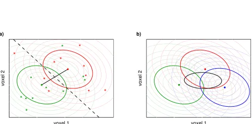
In general, the distinctness of two distributions can be quantified using an information-theoretic measure, the Kullback–Leibler di-vergenceDKL(Kullback and Leibler, 1951). For two equal-variance
normal distributions (see Fig. 1a), this distinctness can be simply expressed by the squared distance of the class means~µ1 and~µ2,
measured with respect to the within-class covarianceΣ,
voxel 1
voxel 2
a)
voxel 1
voxel 2
[image:7.612.54.563.139.390.2]b)
Figure 1: Classification and covariance structure. (a)Data points in voxel activation space that belong to two different classes (red and green stars) can be discriminated using a classification boundary (dashed line) if they come from different distributions (densities indicated by contour lines); here an accuracy of 70 % is achieved. Multivariate normal distributions as shown here are defined by their expectation values (red and green center bullets) and covariance structure (visualized by the strong red and green ellipse-shaped 1σ-lines). In this case, the
discriminability of the two distributions is completely characterized by the Mahalanobis distance∆, the distance of the distribution centers (black line) measured in standard deviations; here∆=1.5. (b)The discriminability of three or more classes is characterized by the magnitude of the between-class covariance (black ellipse) compared to the within-class covariance (colored ellipses). This magnitude can be quantified e.g. by the diagonal diameter of the between-class covariance ellipse measured in standard deviations of the within-class distribution. (Note that the between-class covariance ellipse does not correspond to the 1σ-line of a multivariate normal distribution,
where0 denotes transposition.∆is calledMahalanobis distance (Ma-halanobis, 1936).1
The highest possible mean classification accuracy, achieved by a linear classifier based on perfect knowledge of~µ1,~µ2, and Σ (see
Hastie et al., 2009), can be derived theoretically; it is
αopt =Φ
∆
2
, (3)
whereΦ denotes the cumulative distribution function of the stan-dard normal distribution. If the classifier has been trained on a lim-ited amount of data, imprecise estimation of the distribution pa-rameters leads to worse mean classification performance, but still the mean accuracy α is a monotonically increasing function of ∆,
starting from a chance level of 50 % and saturating for large ∆ to-wards 100 % (for approximate formulas see Wyman et al., 1990).
In contrast to the expected accuracy α estimated by the
classifier-based approach, the equivalent quantity ∆ directly characterizes the multivariate data structure. Other than the accuracy, its esti-mate does not depend on the internals of a particular classification algorithm and it does not saturate for stronger effects. Moreover, it is the multivariate generalization of a standard univariate measure of effect size, Cohen’sd(Cohen, 1988).
2.2
The Multivariate General Linear Model
The multivariate normal distribution model for two-class data (Eq. 1) is a special case of the multivariate general linear model (MGLM),
Y =XB+Ξ. (4)
The equation has the same form as for the GLM underlying univariate fMRI analyses (Friston et al., 1995; Kiebel and Holmes, 2007), except that here the measured data Y is not a time series column vector but of an n×p matrix specifying the signal at n
different time points inpvoxels simultaneously. The design matrix
X specifies time series (columns) for each of the q regressors and remains unchanged from the univariate case. Accordingly, the parameter matrix B is of size q× p and describes the strength of the contribution of each of the q regressors to the signal within each of the p voxels. Finally, each of the n rows of the error term
1The same two-class model underlies linear discriminant analysis.
Ξ is a sample from a p-dimensional normal distribution, N(0,Σ). The following calculations are based on the premise that the rows ofΞare mutually uncorrelated. Since fMRI data are characterized by serial correlations, we assume that they have been removed by a standard whitening procedure during preprocessing (Glaser and Friston, 2007).
The two-class model (Eq. 1) can be written in the form of the MGLM by including two regressors, such that X contains a 1 in the first column for each data point belonging to class 1, a 1 in the second column for each data point belonging to class 2, and zeros otherwise. The two rows of B then correspond to vectors~µ1 and
~µ2.
In GLM-based fMRI analyses,contrast matrices C are used to select specific components out of the total space of effects that the respec-tive model can describe. Each contrast matrix defines a univariate null hypothesis of the formC0B = 0, i.e. the statement that a GLM parameter or a linear combination of parameters is zero, and forms the basis for the computation of a t or F statistic used to test that hypothesis. The same logic applies to the MGLM, only that now the parameters inBbelonging to one regressor are vectors acrossp
voxels, and the specified null hypotheses are multivariate null hy-potheses. If contrasts are used to select partial effects correspond-ing to scorrespond-ingle factors and interactions in a factorial design, this leads to a decomposition or ‘analysis’ of variance (ANOVA) in the case of the GLM and to a multivariate analysis of variance, MANOVA, in the case of the MGLM.
The formal development is again identical in both cases (cf. Kiebel and Holmes, 2007).2 The contrast matrixC is used to separate the parameters of the full model into two parts,
B =B0+B∆ (5)
with
B∆ =C0−C0B =CC−B and B0= B−B∆. (6)
B0describes a reduced model corresponding to the null hypothesis
C0B = 0, andB∆ a possible deviation from this reduced model. In the case of two classes of trials modeled by two regressors and a contrastC = (−1 1)0, B∆ =~µ2−~µ1describes the difference of the
multivariate activation patterns between these classes.
The between-class covariance, i.e. the part of the total covariance of
the data that is accounted for by the class difference, is given by
1
n B
0
∆X0XB∆, (7)
while the within-class covariance is identical to theerror covariance,
1
n
Ξ0Ξ
=Σ. (8)
The size of the multivariate effect is the magnitude of the between-class covariance compared to the within-between-class covariance (Fig. 1b). Since both are p×p matrices, there are different ways to express this comparison in a single number; we choose
D =trace
1
nB
0
∆X0XB∆ Σ−1
, (9)
because in the two-class case it has a simple relationship to the Ma-halanobis distance:
D = 1
4∆
2 · n1+n2
n , (10)
wheren1andn2are the number of data points for class 1 and 2,
re-spectively. We call this measurepattern distinctnessbecause it quan-tifies how distinct different multivariate patterns appear relative to the uncertainty induced by the error.
But the MGLM and the pattern distinctness D are more than just a different way to consider the two-class model. The MGLM can be used with regressors of arbitrary form, i.e. they can be simple indicators for two or more classes of trials, indicator variables con-volved with the hemodynamic response function, or general para-metric regressors where there are no classes.
This allows to apply the MGLM directly to the measured fMRI sig-nal, while a classifier might have to be applied to (run-wise) GLM parameter estimates ˆB in order to provide clear ‘class identities’ for the data points being entered. Moreover, modeling directly the data allows to estimate the ‘within-class’ covariance, which is actu-ally the error covariance Σ, on avolume-by-volume basis, leading to a precise estimate.
case of an interaction of several experimental factors. In short, by using the MGLM the full analytical power of complex factorial de-signsbecomes available to multi-voxel pattern analysis.
Just as the Mahalanobis distance ∆ characterizes the multivariate data structure in the two-class case, the pattern distinctnessD ful-fills this function for the general case of a partial effect defined by a contrastC within an experimental design described by a design matrixX. In contrast to the classification accuracy,D(C)has a clear interpretation as it quantifies the amount of multivariate variance (Cohen, 1982) explained by the effect, measured in units of the error variance.
2.3
Cross-validated MANOVA
The Maximum-Likelihood fit of an MGLM to a given data set is achieved by Least Squares:
ˆ
B=X−Y and Ξˆ =Y−XBˆ. (11)
The straightforward estimate of the pattern distinctness D based on this fit is identical to theBartlett–Lawley–Hotelling trace:
TBLH =trace(H E−1). (12)
Here
H = Bˆ0∆X0XBˆ∆ and E=Ξˆ0Ξˆ (13)
are the hypothesis and error matrices of sums of squares and cross-products. In the univariate case (p =1),HandEare simple sums of squares and the ratioF = H/E· fE/fH gives the ANOVA statistic
with degrees of freedom fH =rankXCand fE =n−rankX.
Along with Wilks’ Λ (cf. Haynes and Rees, 2005a), the Bartlett– Lawley–Hotelling trace TBLH is one of the standard test statistics
used in multivariate statistics (MANOVA, canonical correlation analysis, etc.; see Timm, 2002). As an estimator of D, however, it is severely biased. An intuitive explanation is that TBLH is a
(generalized, squared) distance. Since the estimates cannot be negative, if D is zero or small, estimation errors mostly increase the estimate. Or from a model evaluation perspective, H can be seen as comparing (‘correlating’) the estimate of the contrast effect on the data, XBˆ∆, with itself, leading to an overestimation of the
effect.
cross-validation. The estimate ofDin thelth cross-validation fold,
ˆ
Dl =trace(Hl E−1l ), (14)
combines ˆB∆ computed from data of thelth (‘left out’ or ‘test’) run on the right-hand side with its values from the other (‘training’) runs on the left-hand side:
Hl =
∑
k6=lˆ
B0∆ k
X0XBˆ∆ l and El =
∑
k6=lˆ
Ξ0Ξˆ
k, (15)
where braces with subscript indicate that the expression has to be evaluated using data from the respective run. The complete cross-validated estimate ofD is then the mean of the per-fold estimates
ˆ
Dl. After additionally correcting a multiplicative bias ofE−1in
esti-mating(nΣ)−1, the final unbiased estimator of the pattern distinct-nessDbecomes (see Appendix A)
ˆ
D= (m−1) fE−p−1 (m−1)n ·
1
m
m
∑
l=1ˆ
Dl. (16)
While the Bartlett–Lawley–Hotelling trace TBLH is useful as a test
statistic to determine whether the observed effect is significantly different from zero, its cross-validated version ˆD can serve the same purpose, but additionally provides an unbiased estimate of the size of the effect. Such a characterization of the effect inde-pendent of the amount of data available or its partitioning into ‘training’ and ‘test’ sets enables interpretation and potentially facilitates cross-study comparisons and power analyses (cf. Cohen, 1988). However, the estimated effect size D itself does of course depend on the specific design matrixXused (e.g. number of trials, type of regressors), and may depend on the number of voxels p
included in the analysis.
A small modification is advisable for the purpose of topologically specific inference using a statistical parametric map of ˆD-values. Since searchlight spheres centered near the boundaries of the brain mask contain fewer voxels and the variance of the null distribution of ˆDis approximately proportional to p(see Appendix B), the map has an inhomogeneous null variance. We therefore recommend to use statistical parametric maps of thestandardizedpattern distinct-ness
ˆ
Ds = √1
pDˆ, (17)
2.4
Simulation
The statistical properties of ˆD were investigated using artifi-cial data sets approximately simulating an fMRI experiment. It
comprised m = 4 runs of n = 512 volumes each. There were
n1 = n2 = 16 trials per run for each condition, each lasting for
one volume, such that the design matrix consisted of indicator variables for the two conditions and a constant regressor. Data were generated according to the MGLM equation (Eq. 4) with serially uncorrelated errors, i.e. the simulation refers to data after the whitening preprocessing step. The error covariance was set to Σ = I without loss of generality (cf. Appendix A). The contrast considered was C = (−1 1 0)0. For each choice of simulation parameters (true effect size D and dimensionality p), 10, 000 data sets were generated.
For each artificial data set, additionally the empirical accuracy a
was determined for classification of run-wise parameter estimates ˆ
β1· and ˆβ2· (p-dimensional vectors) as well as for classification of
single-trial volumes, in each case using a linear soft-margin sup-port vector classifier (Cortes and Vapnik, 1995), in the implementa-tion of the LIBSVM library (Chang and Lin, 2011).
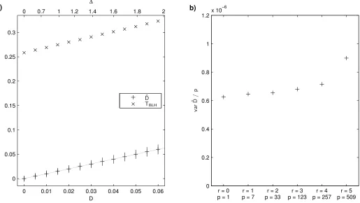
Fig. 2a shows ˆD and TBLH as a function of D for p = 123 voxels,
corresponding to a searchlight radius of 3 voxels. The simulation demonstrates the extreme estimation bias ofTBLH, and confirms the
theoretical result that ˆDis an unbiased estimator ofD.
Fig. 2b shows the sampling variance of ˆDunder the condition that there is no true effect (D = 0), as a function of p. It demonstrates that the ratio var ˆD/p is approximately constant for small to moderate values of p. This supports the theoretical expectation of proportionality between null variance and dimensionality, which means that the standardized pattern distinctness ˆDs = √1pDˆ is a
suitable statistic to construct statistical parametric maps.
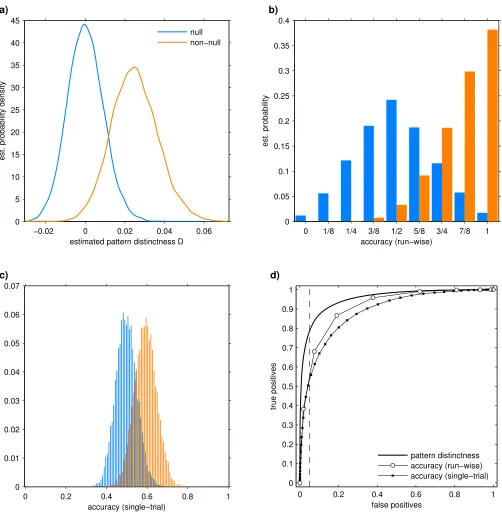
The usefulness of the pattern distinctness ˆD and the empirical ac-curacyaas a statistic to distinguish data sets with a true underlying effect from those with a null effect is investigated in Fig. 3. The cho-sen non-null effect ofD=0.025 can be considered ‘large’ if the cor-responding∆=1.26 is compared to Cohen’s recommendations for
0 0.01 0.02 0.03 0.04 0.05 0.06 0
0.05 0.1 0.15 0.2 0.25 0.3
D
a)
ˆ D TBLH
0 0.7 1 1.2 1.4 1.6 1.8 2 ∆
0 0.2 0.4 0.6 0.8 1 1.2
x 10−6
va
r
ˆ D/
p
b)
r = 0 p = 1
r = 1 p = 7
r = 2 p = 33
r = 3 p = 123
r = 4 p = 257
[image:14.612.53.568.182.472.2]r = 5 p = 509
Figure 2: Simulation results: Statistical properties. (a) The cross-validated and na¨ıve estimates of D, ˆD and TBLH, as a function ofDforp=123 voxels. Values of ˆDare shown with a marker (+) indicating the mean and a
vertical line for the interquartile range of the sampling distribution, values ofTBLHonly with a marker (×). The
identity line ˆD=Dis shown in gray. For reference, the upper horizontal scale gives the corresponding values of the Mahalanobis distance∆. The plot confirms that ˆDis an unbiased estimator ofD, while the Bartlett–Lawley– Hotelling trace TBLHis strongly biased. (b)The ratio var ˆD/pforD = 0, as a function of the number of voxels
−0.02 0 0.02 0.04 0.06 0 5 10 15 20 25 30 35 40 45
estimated pattern distinctness D
est. probability density
a)
null non−null
0 1/8 1/4 3/8 1/2 5/8 3/4 7/8 1
0 0.05 0.1 0.15 0.2 0.25 0.3 0.35 0.4 accuracy (run−wise) est. probability b)
0 0.2 0.4 0.6 0.8 1
0 0.01 0.02 0.03 0.04 0.05 0.06 0.07 accuracy (single−trial) est. probability c)
0 0.2 0.4 0.6 0.8 1
[image:15.612.60.562.57.577.2]0 0.1 0.2 0.3 0.4 0.5 0.6 0.7 0.8 0.9 1 false positives true positives d) pattern distinctness accuracy (run−wise) accuracy (single−trial)
problem, but still the sampling distributions for null- and non-null effect appear to overlap more than for ˆD.
The same observation is presented in a more precise way in Fig. 3d in the form of a ‘receiver operating characteristic’ diagram (ROC, see also Kriegeskorte et al., 2006). If a data set is determined to show an effect based on comparison with a threshold, the trade-off between false and true positive rate can be adjusted by choosing the threshold value. The ROC curves show that in this simulation ˆD
achieves a higher true positive rate than both run-wise and single-trial classification accuracies for arbitrary given false positive rate. Though this result suggests that hypothesis tests based on ˆD may be more powerful than tests based ona, their relative performance will depend on the exact structure of the data set and the chosen comparison; see Sec. 3 for an example where a shows statistically stronger effects than ˆD.
2.5
Pattern stability
A common variation of classifier-based pattern analysis is ‘cross-decoding’ (cf. Haynes and Rees, 2005b), i.e. training a classifier on one pair of classes and testing it on another pair of classes. This method is typically applied in a factorial design, where the two pairs of classes refer to the same factor but under different levels of a second factor (see next section for an example). Cross-decoding is therefore the complement of an interaction analysis: while the latter attempts to show that a pattern difference changes under an additional manipulation, cross-decoding attempts to show that it remainsstable. This approach can be translated into the framework presented here; since our measure of multivariate effect is based on ‘correlating’ parameter estimate differences ˆB∆ between ‘training’ and ‘test’ runs (Eq. 15), it is also possible to apply it to estimate differences computed for different contrasts.
However, the explicit computation of such a modified form of the pattern distinctnessDis not necessary. The degree of stability of a multivariate effect E across the levels of another experimental fac-tor A can be quantified by combining the multivariate measures of the effect E and the interaction E×A. Under the hypothesis of max-imal inconsistency (mutual orthogonality) of patterns across theL
levels of A it holds
D(E) = 1
L−1 D(E×A) (18)
symbol for the set complement (‘\’) to denote the complement of an interaction (‘×’), we can define
D(E\A) = D(E)− 1
L−1 D(E×A) (19)
as the multivariate measure of pattern stability. It is 0 for maximal pattern inconsistency and attains its maximum value of D(E) for zero interaction, i.e. maximum pattern stability.
The expression can be interpreted such that the total amount of variance accounted for by the effect E is reduced by that part that is inconsistent across the levels of A, quantified by the strength of the interaction. Applied to estimates ˆD of the multivariate effects, it can be used as a test statistic to reject the null hypothesis of maxi-mal pattern inconsistency and thereby provide evidence for pattern stability.
3
Application
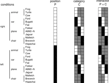
In order to demonstrate the use of our measure of pattern distinct-ness, we reanalyzed the data of Cichy et al. (2011). In this study, renderings of three-dimensional object meshes were presented to subjects either to the left or the right of a central fixation dot. The objects belonged to four different categories with three exemplars for each category, resulting in 24 experimental conditions (see Fig. 4). Images were presented in mini-blocks of six different views of the same object, at a rate of one view per second. There were four mini-blocks per condition in each of the five experimental runs. Data were acquired in 412 fMRI volumes per run at a TR of 2 s, with a field of view covering the ventral visual cortex at an isotropic res-olution of 2 mm. Volumes were slice-time corrected, realigned and normalized to the MNI template. Thirteen subjects participated in the experiment, but the data of one were discarded because of strong head movements. The data of each subject were modeled with one design matrix per run, each comprising regressors for the 24 conditions. Regressors were composed of canonical HRFs time-locked to each image presentation. Preprocessing, construction of the design matrix, and removal of serial correlations were per-formed in SPM8 (http://www.fil.ion.ucl.ac.uk/spm/), further analysis in custom SPM-based MATLAB code (The Mathworks, Natick).
Frog Turtle Cow Ford Bugatti Fiat Fokker A6M2−N Jaguar Malletch Breverch Hopechai Frog Turtle Cow Ford Bugatti Fiat Fokker A6M2−N Jaguar Malletch Breverch Hopechai animal
car
plane
chair
animal
car
plane
chair right
left
conditions
position P
category C
[image:18.612.117.488.206.487.2]interaction P × C
Figure 4: Experimental conditions and contrasts. Renderings of twelve different objects belonging to four dif-ferent categories were shown left and right of a fixation dot. The 24 resulting conditions were examined in the form of three contrasts corresponding to the main effects of position (P) and category (C), and their interaction (P×C). The associated contrast matricesCare shown in grayscale, where white stands for a value of 1, black for
the main effects of P and C, as well as the interaction P × C; the corresponding contrast matrices are shown in Fig. 4.
Using a searchlight of radius 4 voxels (p = 257 voxels), for each searchlight position we computed MGLM parameter estimates ˆB
and residuals ˆΞ(Eq. 11). The respective contrast was applied to ob-tain ˆB∆ =CC−Bˆ. Performing a leave-one-run-out cross-validation, for each fold l = 1 . . .m hypothesis and error matrices Hl and El
were computed (Eq. 15) and from them the fold-wise estimate of pattern distinctness ˆDl (Eq. 14). The per-fold estimates were then
combined into the final unbiased estimate of pattern distinctness ˆD
(Eq. 16). The result was converted into a statistical parametric map, SPM{Dˆs}, of standardized pattern distinctness (Eq. 17). Maps
com-puted for each subject and contrast separately were subsequently smoothed with a Gaussian kernel of 6 mm FWHM.
The application of standard second-level statistics includingt-tests to cross-validated MVPA measures has been discussed critically by Stelzer et al. (2013). We instead followed their approach to perform a group-level permutation test by combining single-subject permu-tation values selected independently in each subject. These single-subject permutations were generated by a sign-permutation pro-cedure adapted for cross-validated MANOVA, described in App. D. With m = 5 runs, there were 24 = 16 single-subject permuta-tions and 1612 = 2.8·1014 combined permutations, out of which 100, 000 were randomly selected. The group-level test statistic was the standardized pattern distinctness ˆDs averaged across subjects.
Statistical results were corrected for multiple comparisons at the voxel level by using the permutation distribution of the maximum statistic across voxels (Nichols and Holmes, 2002).
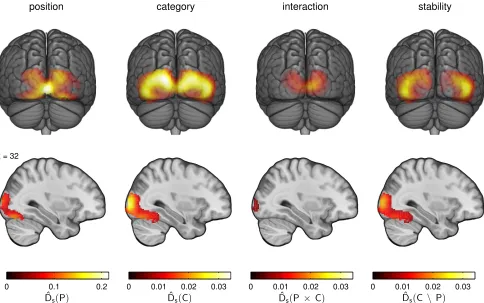
The results are shown in Fig. 5. The pattern distinctness for the three computed contrasts obtains values significantly different from zero over large areas of the visual cortex, with maxima
exhausting the number of computed permutations, P ≤ 10−5
(corr.). The same holds for the measure of pattern stability ˆ
Ds(C\P) = Dˆs(C) −Dˆs(P×C) which quantifies the degree of
stability of category-specific patterns across the two positions (Eq. 19), i.e. indicates the presence of position-invariant category information. The effect sizes reach maxima of ˆD = √pDˆs = 3.45
position
x = 32
0 0.1 0.2
category
0 0.01 0.02 0.03
interaction
0 0.01 0.02 0.03
stability
[image:20.612.65.549.143.446.2]0 0.01 0.02 0.03 ˆDs(P) ˆDs(C) ˆDs(P× C) ˆDs(C \ P)
Figure 5: Analysis results. The results of cvMANOVA in the form of statistical parametric maps of the standard-ized pattern distinctness ˆDs, averaged across twelve subjects, for four different multivariate effects. The maps are
shown on a 3D rendering of the ICBM152 template brain and on a sagittal slice atx= 32. The highlighted areas are those where the multivariate effect was statistically significant at a level of P ≤ 0.05, corrected for multiple comparisons. The multivariate main effect of position (P) is strongest over primary visual cortex, while the main effect of category (C) extends from middle and superior occipital gyrus into the fusiform gyrus. The multivariate interaction of these two factors (P×C) is again mainly confined to primary visual areas. In addition to the three standard contrasts (see Fig. 4), the fourth column shows the difference in effect size between the main effect of category and the interaction, ˆDs(C\P) = Dˆs(C)−Dˆs(P×C). This difference quantifies the degree of stability
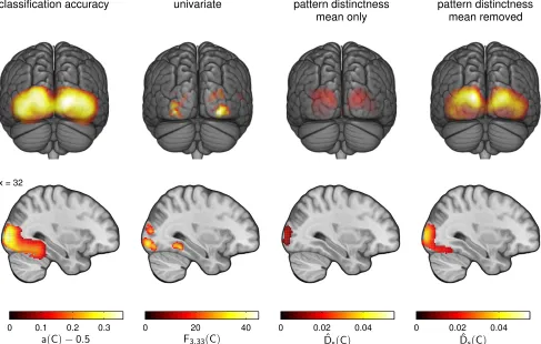
To compare cross-validated MANOVA with established analysis methods, we also computed classification accuracies and mass-univariate statistical parametric maps. However, please note that classification accuracy is not defined for an interaction effect and there is no analogue of ‘pattern stability’ for univariate analysis. Cross-validated accuracies were determined using an SVM to clas-sify run-wise parameter estimates. Accuracy maps were smoothed with a Gaussian kernel of 6 mm FWHM before entering statistical assessment, which was based on a permutation procedure analo-gous to that applied to ˆD, exchanging labels between conditions. Statistical significance of accuracies averaged across subjects was again assessed by comparing actual values with the permutation distribution of the maximum statistic, estimated by 100, 000 times randomly combining single-subject permutations. Additionally, we computed the univariate second-level SPM{F}applied to first-level contrast images (smoothed as above), statistically assessed in SPM8 by standard familywise error correction based on random field theory.
The results for ‘category’ are shown in Fig. 6. The classification analysis gives a similar picture of the localization of category in-formation as cvMANOVA. In contrast to the simulation results of Sec. 2.4, statistical power of the test based on the classification ac-curacy a appears to be higher than that based on the pattern dis-tinctness ˆD. Univariate effects are observed in areas consistent with the multivariate analyses but turn out to be much weaker. To en-sure that this difference is not just due to different statistical meth-ods, we repeated the cross-validated MANOVA, but set all param-eter estimates within each searchlight to their mean before mul-tivariate analysis. The results (Fig. 6) are much weaker and espe-cially fail to uncover category effects in fusiform gyrus. By con-trast, cvMANOVA computed on parameter estimates from which the mean was removed for each searchlight location separately give only slightly weaker results than the original analysis, indicating that the observed effect has a predominantly non-univariate char-acter.
4
Discussion
classification accuracy
x = 32
0 0.1 0.2 0.3
univariate
0 20 40
pattern distinctness mean only
0 0.02 0.04
pattern distinctness mean removed
[image:22.612.63.550.181.491.2]0 0.02 0.04 a(C)−0.5 F3,33(C) ˆDs(C) ˆDs(C)
4.1
Nonnormality
As stated above, our data model assumes multivariate normally distributed additive errorsΞ, which is the natural multivariate gen-eralization of the assumption underlying standard univariate fMRI analyses. The theoretical justification for the normality assumption is that the error term captures all those aspects of the operation of the brain and the MR scanner which do not systematically occur in the experiment and therefore cannot be modeled explicitly. Because these processes are likely to be high-dimensional and their many small contributions add up, according to the central limit theorem the error can be expected to be normally distributed. Since this the-orem generalizes to the multivariate case (see Timm, 2002), the jus-tification also holds for the MGLM. In practice, residuals of prop-erly constructed models in fMRI do appear to be approximately normally distributed (Kruggel and Cramon, 1999), and univariate analyses which depend on this assumption have proven to be suc-cessful and reliable.
A within-class multivariate normal distribution is also the model underlying the standard parametric approach to classification, LDA, which was successfully used in several early MVPA studies (Carlson et al., 2003; Cox and Savoy, 2003; Haynes and Rees, 2005a, 2005b). However, as Hastie et al. (2009) state, optimal performance of linear classifiers is not bound to multivariate normality; it extends to the family of distributions that are characterized by a mean pattern ~µ, a covariance matrix Σ and a monotonically
decreasing functiong(d)such that the density is
p(~x) ∝ g(~x−~µ)0 Σ−1(~x−~µ)
, (20)
theelliptical distributions(see Fang et al., 1990). Since in this family of distributions the probability of a data point is a function of the Mahalanobis distance from the distribution center, the argument translates to our measure: Quantifying the distinctness of distribu-tions using the Mahalanobis distance and our generalizationD is still appropriate for distributions heavier- or thinner-tailed than the multivariate normal, as long as they fall within the elliptical family.
4.2
Nonlinearity
An advantage of classifiers might be seen in the fact that kernel-based methods (Boser et al., 1992) allow for nonlinear classification. However, the established assumptions about the statistical struc-ture of fMRI data that are built into standard univariate analyses do not give reason to expect a gain from nonlinear algorithms. On the contrary, a nonlinear classifier may confound different partial effects in a factorial design that can be differentiated by the multi-variate linear approach proposed in this paper.
For this it is important to note that nonlinear optimal classification boundaries do not arise from a nonlinearity of the patterns, but from a differenterrorcovariance structure within different classes. While the pattern characterizing a class has presumably been generated by a process of nonlinear neural dynamics (cf. Haken, 1995), the pattern vector ~µ itself is a point in voxel activation
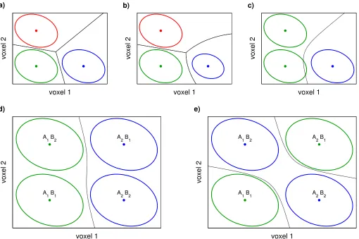
space and therefore does not allow for nonlinear structure. If the data points belonging to each class are distributed according to the same elliptical distribution with different means (Fig. 7a), optimal classification boundaries are piecewise linear. Nonlinear boundaries (Fig. 7b) arise if this ‘homoscedasticity’ assumption is violated. In the simplest case, classification boundaries become (hyper-) paraboloid (quadratic discriminant analysis; see Hastie et al., 2009).
A violation of homoscedasticity is not to be expected as long as the within-class variance consists only of the contributions of complex unknown background processes described by the additive error term Ξ in the MGLM, and all systematically occurring effects are explicitly modeled. The most likely cause of heteroscedasticity is therefore insufficient modeling of the data. An example is shown in Fig. 7c: A situation where there are actually three different patterns involved has been modeled by two classes, disregarding the dis-tinction between two of the patterns. Because of this, the two result-ing classes have a different covariance structure, and one of them is also no longer meaningfully characterized by a single pattern vec-tor. Consequently, the classification boundary becomes nonlinear. However, such a ‘pooling’ of data from different experimental con-ditions, which is sometimes used in classifier-based MVPA studies utilizing more complex designs (e.g. Cichy et al., 2012; Momenne-jad and Haynes, 2012), can be avoided in the MGLM framework: The design matrix should always be constructed such that it mod-els all the systematic experimental effects; and the selection of par-tial effects is implemented by choosing the correct contrast.
voxel 1
voxel 2
a)
voxel 1
voxel 2
b)
voxel 1
voxel 2
c)
voxel 1
voxel 2
d)
A 1 B1 A
1 B2
A 2 B2 A
2 B1
voxel 1
voxel 2
e)
A 1 B1 A
1 B2
A 2 B2 A
[image:25.612.55.565.107.446.2]2 B1
Figure 7: Causes for and misinterpretation of nonlinear optimal classification. (a) If the data adhere to the assumptions of the multivariate linear model which implies that all classes are characterized by the same ellip-tical distribution (red, green and blue ellipses) with the same variance (homoscedasticity), optimal classification boundaries (black lines) are also piecewise linear. (b)These boundaries become nonlinear if the variance differs between classes (violation of homoscedasticity), which however is incompatible with the assumption of additive noise made by the MGLM (Eq. 4). (c)A more realistic scenario for how heteroscedasticity and thereby nonlin-earity may arise is that one class (green) is actually a compound of two or more patterns (greenandred in panel a). (d)Such compound classes occur for instance in the decoding of single factors in a multifactorial design. In the case illustrated here there are two factors A and B with two levels each. The four resulting conditions are pooled into two classes according to the levels of the factor A (green for A1, blue for A2). The clear separation of
these classes by the classification boundary is consistent with the fact that there is a multivariate main effect of factor A. (e)However, a nonlinear classifier would also be able to separate data pooled according to the levels of factor B (green for B1, blue for B2), though there is no multivariate main effect of factor B. By contrast, the
demonstrates that the application of a nonlinear classifier to pooled data can even be misleading. In this example, the four different patterns belong to the four cells of a 2 × 2 factorial design, and the two classes encode either the two levels of factor A (6d) or of factor B (6e). The success of classification in the second case might be interpreted such that there is an effect of factor B, since data pooled according to the levels of this factor can be nonlinearly separated. However, from a MANOVA perspective the situation shown is characterized by an interaction A×B and a main effect of factor A, but no main effect of factor B. The MGLM framework is therefore able to describe the structure of the data in a more detailed way exactly because it is linear.
4.3
Insufficient data
A limitation of MVPA measures like Mahalanobis distance or LDA classification accuracy that use an explicit probabilistic model of the fMRI data (a ‘generative’ model) is that in a high-dimensional space spanned by a large number of voxels the number of data points is not sufficient to properly estimate the within-class
covari-anceΣ. In such a case, using a ‘discriminative’ model, which does
not describe the distribution of the data points but only allows to assign them to classes, may be necessary.
This limitation holds for the cross-validated MANOVA method presented in this paper, too. However, the situation is vastly improved compared to methods applied to run-wise parameter estimates because the MGLM operates on the level of single volumes. Moreover, it makes even better use of the data than trial-wise classification. Where a classifier would assess the within-class variation based on the volumes belonging to the two classes of trials involved, the error covariance of the MGLM is estimated using the residuals of the full model across the whole length of the recording. Since within the cross-validation scheme (Sec. 2.3) the error covariance estimate in each fold is based on data from all but one of the m runs, a non-singular estimate E is obtained as soon as(m−1) fE ≥ p, where the number of error degrees of freedom
is given by the number of volumes per run minus the number of linearly independent regressors. For searchlight-based MVPA of typical fMRI studies not just a non-singular but a good estimate should be possible for radii up to 4 (p =257).
or reduction of dimensionality via principal component analysis as a preprocessing step (cf. Carlson et al., 2003) or via built-in model constraints (Worsley et al., 1997) are possible solutions, but with the drawback that the resulting estimator is biased. A better approach to extend the field of application of cvMANOVA might therefore be to develop a model of the local error covariance structure, e.g. based on voxel distance or tissue types.
5
Conclusion
In this paper we have introduced a measure for use in searchlight-based MVPA studies, the pattern distinctness D, as a replacement of the often employed measure of accuracy. Instead of quantifying the performance of a classifier, our measure is based on the multi-variate extension of the general linear model (the MGLM). It there-fore does not depend on a particular classifier and its parameters, but directly characterizes the structure of fMRI data by quantifying the amount of multivariate variance explained by a given effect, in terms of the error variance. The measure is related to standard MANOVA statistics, but cross-validation is applied to obtain an un-biased estimate ˆDof the size of the effect. Other than the approach of Friston et al. (2008) that implements Bayesian model selection for the MGLM, our method aims to be a straightforward extension of univariate statistics to the multivariate case.
The MGLM underlying cross-validated MANOVA uses the same design matrix and is analyzed using the same contrast matrices as those used with the GLM, which thereby provide a unified basis for univariate and multivariate analyses. Because it is based on the MGLM, cvMANOVA can be used for two or more classes of tri-als but tri-also with parametric regressors, and ˆD can quantify the multivariate effect defined by any estimable contrast. This way it becomes possible to use MVPA to investigate main effects in a fac-torial design as well as interactions, i.e. the question whether the
pattern difference between two or more levels of one factorchanges
Appendix
A
Estimation bias
The expectation value of ˆDl is
hDˆli =trace D
Hl El−1 E
=tracehHli hE−1l i
, (A.1)
because Hl and Elare uncorrelated, since ˆB∆ and ˆΞarise from
mu-tually orthogonal projections. For the hypothesis matrix,
hHli =
∑
k6=lˆ
B0∆ k X0XBˆ∆ l =
∑
k6=lˆ
B∆0 k X0XBˆ∆ l,
(A.2) because the two braces are computed from data of different runs, and sincehBˆ∆i =B∆,
hHli= (m−1)B∆0 X0XB∆. (A.3)
The error matrix follows a Wishart distribution (Timm, 2002),
El =
∑
k6=lˆ
Ξ0Ξˆ
k ∼ Wp(Σ,(m−1) fE), (A.4)
and therefore the expectation of its inverse is
hE−1l i = 1
(m−1) fE−p−1Σ −1
. (A.5)
Consequently,
hDˆli =
(m−1)n (m−1) fE−p−1
trace
1
nB
0
∆X0XB∆Σ−1
, (A.6)
where the trace term is identical to the definition of D(Eq. 9), and therefore
hDˆi=
*
(m−1) fE−p−1
(m−1)n ·
1 m m
∑
l=1 ˆ Dl +=D. (A.7)
B
Null distribution
In order to calculate the variance of ˆDlforB∆ =0, we first
approx-imateE−1l by its expectation value (Eq. A.5), so that
ˆ
Dl ≈
1
(m−1) fE−p−1 trace
(Hl Σ−1) for p(m−1) fE.
For the trace holds
trace(Hl Σ−1) =trace
∑
k6=lˆ
B0∆ k X0XBˆ∆ l·Σ−1 !
, (B.9)
and since
ˆ
B∆ =CC−X−Y =CC−X−Ξ (B.10)
forB∆ =0,
trace(HlΣ−1) =
∑
k6=ltrace
Ξ0
X0−CC− k
X0XCC−X−Ξ l·Σ−1.
(B.11) Under the trace, Σ−1 acts as a normalization of Ξk and Ξl, so that
we can chooseΣ=I (the identity matrix) without loss of generality.
Without the intermediate matrix expressions, trace(Ξ0kΞl) is the sum of p inner products of two different n-dimensional random vectors each, with elements independently distributed asN(0, 1). That is, it is the sum of p n product-normally distributed random variables. Due to the additional matrices forming projection operators, the inner products are actually calculated in an fH
-dimensional subspace (due to the contrast C) of a q-dimensional space (due to the design matrixX), and the trace becomes a sum of
p fH independent product-normally distributed random variables,
each of unit variance. Therefore
vartrace(Hl Σ−1)
= (m−1) p fH, (B.12)
and
var ˆDl ≈
(m−1)p fH
((m−1) fE−p−1)2
. (B.13)
Moreover, since due to the central limit theorem sums of indepen-dent random variables tend towards the normal distribution, we can expect ˆDl to be approximately normally distributed around 0
for largerp fH (rule of thumb:>30).
Due to complex statistical dependencies between the cross-validation folds the simple extension, var ˆD ≈ p fH/((m −
1)m n2), can only be a very rough approximation. However, the proportionality topshould hold well forp(m−1) fE.
C
Pattern stability
design, but not A. It therefore consists of a ‘contrast element’cthat is replicated across the levels ofA
C = c c .. . c . (C.14)
We denote asCi the partial contrasts of C, i.e versions of C where
all the replications of c are replaced by zeros, except for the one associated with leveli=1 . . .Lof factor A.
The matrix to extract the parameter difference B∆ associated with
effect E from the parametersBof the full model (Eq. 6) has the form of a Kronecker product
CE =CC− = 1 L
1 1 . . . 1 1 1 . . . 1
..
. ... . .. ... 1 1 . . . 1
⊗ (cc−), (C.15)
while the corresponding matrix for the interaction E×A has the form
CE×A = 1
L
(L−1) −1 . . . −1
−1 (L−1) . . . −1
..
. ... . .. ...
−1 −1 . . . (L−1)
⊗ (cc−). (C.16)
The condition of maximal inconsistency of the multivariate effects associated withcacross the levels of A is defined by the mutual or-thogonality of the partial effects,CiCi−B. In this case, contributions
due to the off-diagonal elements of the matrices in the previous two expressions become zero, and consequently
D(E) = 1
L−1 D(E×A). (C.17)
The resulting measure of pattern stability,
D(E\A) = D(E)− 1
L−1 D(E×A), (C.18)
can be considered a special form of the pattern distinctness D
which is defined by an extraction matrix
CE\A =CE− 1
L−1 CE×A = 1
L−1
0 1 . . . 1 1 0 . . . 1
..
. ... . .. ... 1 1 . . . 0
⊗ (cc−).
In this form the analogy to cross-decoding becomes apparent: The measure only comprises terms that combine patterns fromdifferent levelsof the factor A.CE\A cannot be written as a productCC−and therefore does not correspond to a contrast, butD(E\A)shares the statistical properties of the pattern distinctnessD.
D
Permutation statistics
As shown in Appendix A, if there is no true effect the single-fold estimate ˆDlis asymptotically normally distributed around 0.
How-ever, the approximation we were able to derive for var ˆDl does not
simply translate to ˆD itself, and we do not have any results for higher order moments. Combined with the fact that empirical data will not exactly adhere to the assumption of multivariate normality underlying these derivations, we recommend to use a permutation procedure for the assessment of a statistically significant deviation from a null hypothesis, H0 : D =0.
A permutation test (Good, 2005; Lehmann and Romano, 2005; Nichols and Holmes, 2002) is a null hypothesis test that makes only weak distributional assumptions, and derives the critical value of a test statistic by a computational procedure that utilizes the given sample. The method is based on the symmetries of the distribution of the data (or derived statistics) under H0, which make it possible
to generate a set of artificial samples consistent with the null hypothesis by exchanging (‘permuting’) parts of the original data. The test statistic is computed for all possible permutations, and the null hypothesis is rejected if the actual value of the statistic has an extreme position within the set of permutation values.
In the case of cross-validated MANOVA, we propose to implement permutations at the level of experimental runs beause they can be considered mutually statistically independent. The circumstance that MGLM parametersBare estimated separately for each run and the cross-validation procedure combines parameter estimates from different runs into the measure ˆDleads to the following approach:
Under the null hypothesis D = 0 for a given contrast C, the con-trast parameter estimate ˆB∆ = CC−Bˆ is symmetrically distributed around 0. The resultingsign permutation
ˆ
B∆ k → −Bˆ∆ k (D.20)
does not change the value of ˆD, half of these permutations are re-dundant, leaving an effective number of 2m−1permutations.
For the typical number of runs of an fMRI experiment, the resulting number of permutations is not sufficient to perform a null hypoth-esis test for a single subject at standard significance levels. In this paper, we follow the approach of Stelzer et al. (2013) to construct a group-level permutation distribution by combining permutations independently selected in each subject (see Sec. 3).
Acknowledgements
The authors would like to thank Guillaume Flandin for provid-ing invaluable insights into the innards of SPM8 and Radek Cichy for access to the fMRI data set, Martin Hebart, Kerstin Hackmack, Mar´ıa Herrojo Ruiz, Carsten Bogler, Martin Weygand, Jakob Hein-zle, Stefan Bode, Kai G ¨orgen, and Fernando Ram´ırez for discus-sions, comments, and help, as well as two anonymous reviewers for helpful criticism.
An implementation of the analysis method for use with SPM8 can be obtained from the corresponding author.
References
Abrams, D., Bhatara, A., Ryali, S., Balaban, E., Levitin, D., Menon, V., 2011. Decoding temporal structure in music and speech relies on shared brain resources but elicits different fine-scale spatial pat-terns. Cereb. Cortex 21, 1507–1518.
Blankertz, B., Lemm, S., Treder, M., Haufe, S., M ¨uller, K.-R., 2011. Single-trial analysis and classification of eRP components – a tuto-rial. NeuroImage 56, 814–825.
Boser, B.E., Guyon, I.M., Vapnik, V.N., 1992. A training algorithm for optimal margin classifiers, in: Proceedings of the Fifth Annual Workshop on Computational Learning Theory. ACM, pp. 144–152.
Carlson, T.A., Schrater, P., He, S., 2003. Patterns of activity in the categorical representations of objects. J. Cogn. Neurosci. 15, 704– 717.
Chang, C.-C., Lin, C.-J., 2011. LIBSVM: a library for support vector machines. ACM Trans. Intell. Syst. Technol. 2, 27:1–27:27.
Cichy, R.M., Heinzle, J., Haynes, J.D., 2012. Imagery and perception share cortical representations of content and location. Cereb. Cortex 22, 372–380.
Cohen, J., 1982. Set correlation as a general multivariate data-analytic method. Multivariate Behavioral Research 17, 301–341.
Cohen, J., 1988. Statistical power analysis for the behavioral sci-ences, 2nd ed. Lawrence Erlbaum.
Cortes, C., Vapnik, V., 1995. Support-vector network. Mach. Learn. 20, 273–297.
Cox, D.D., Savoy, R.L., 2003. Functional magnetic resonance imag-ing (fMRI) “brain readimag-ing”: detectimag-ing and classifyimag-ing distributed patterns of fMRI activity in human visual cortex. NeuroImage 19, 261–270.
Edelman, S., Grill-Spector, K., Kushnir, T., Malach, R., 1998. Toward direct visualization of the internal shape representation space by fMRI. Psychobiology 26, 309–321.
Fang, K., Kotz, S., Ng, K., 1990. Symmetric multivariate and related distributions, ed. Chapman; Hall.
Friston, F., Holmes, A.P., Worsley, K.J., Poline, J.-P., Frith, C. D., Frackowiak, R.S.J., 1995. Statistical parametric maps in functional imaging: a general linear approach. Hum. Brain Mapp. 2, 189–210.
Friston, K., Chu, C., Mour˜ao-Miranda, J., Hulme, O., Rees, G., Penny, W., Ashburner, J., 2008. Bayesian decoding of brain images. NeuroImage 39, 181–205.
Friston, K.J., Frith, C.D., Liddle, P.F., Frackowiak, R.S., 1993. Functional connectivity: the principal-component analysis of large (PET) data sets. J. Cereb. Blood Flow Metab. 13, 5–14.
Glaser, D., Friston, K., 2007. Covariance components, in: Friston, K.J., others (Eds.), Statistical Parametric Mapping: the Analysis of Functional Brain Images. Academic Press.
Good, P.I., 2005. Permutation, parametric, and bootstrap tests of hy-potheses, 3rd ed. Springer.
Goutte, C., Toft, P., Rostrup, E., Nielsen, F. ˚A., Hansen, L.K., 1999. On clustering fMRI time series. NeuroImage 9, 298–310.
Haken, H., 1995. Principles of brain functioning: a synergetic ap-proach to brain activity, behavior, and cognition, ed. Springer.
Haxby, J.V., 2012. Multivariate pattern analysis of fMRI: the early beginnings. NeuroImage.
Haxby, J.V., Gobbini, M.I., Furey, M.L., Ishai, A., Schouten, J.L., Pietrini, P., 2001. Distributed and overlapping representations of faces and objects in ventral temporal cortex. Science 293, 2425–2430.
Haynes, J.-D., Rees, G., 2005a. Predicting the orientation of invisi-ble stimuli from activity in human primary visual cortex. Nat. Neu-rosci. 8, 686–691.
Haynes, J.-D., Rees, G., 2005b. Predicting the stream of conscious-ness from activity in human visual cortex. Curr. Biol. 15, 1301–1307.
Haynes, J.-D., Rees, G., 2006. Decoding mental states from brain activity in humans. Nat. Rev. Neurosci. 7, 523–534.
Kahnt, T., Grueschow, M., Speck, O., Haynes, J.-D., 2011. Percep-tual learning and decision-making in human medial frontal cortex. Neuron 70, 549–559.
Kamitani, Y., Tong, F., 2005. Decoding the visual and subjective con-tents of the human brain. Nat. Neurosci. 8, 679–685.
Kiebel, S.J., Holmes, A.P., 2007. The general linear model, in: Fris-ton, K.J., others (Eds.), Statistical Parametric Mapping: the Analysis of Functional Brain Images. Academic Press.
Kriegeskorte, N., Goebel, R., Bandettini, P., 2006. Information-based functional brain mapping. Proc. Natl. Acad. Sci. U. S. A. 103, 3863–3868.
Kruggel, F., Cramon, D.Y. von, 1999. Modeling the hemodynamic response in single-trial functional mRI experiments. Magn. Reson. Med. 42, 787–797.
Kullback, S., Leibler, R.A., 1951. On information and sufficiency. Ann. Math. Stat. 22, 79–86.
Lehmann, E.L., Romano, J.P., 2005. Testing statistical hypotheses, 3rd ed. Springer.
Mahalanobis, P.C., 1936. On the generalised distance in statistics. Proc. Natl. Inst. Sci. India 2, 49–55.
McIntosh, A.R., Bookstein, F.L., Haxby, J.V., Grady, C.L., 1996. Spa-tial pattern analysis of functional brain images using parSpa-tial least squares. NeuroImage 3, 143–157.
Mitchell, T.M., Hutchinson, R., Niculescu, R.S., Pereira, F., Wang, X., Just, M., Newman, S., 2004. Learning to decode cognitive states from brain images. Mach. Learn. 57, 145–175.
Momennejad, I., Haynes, J.-D., 2012. Human anterior prefrontal cortex encodes the “what” and “when” of future intentions. Neu-roImage 61, 139–148.
Nichols, T.E., Holmes, A.P., 2002. Nonparametric permutation tests for functional neuroimaging: a primer with examples. Hum. Brain Mapp. 15, 1–25.
Norman, K.A., Polyn, S.M., Detre, G.J., Haxby, J.V., 2006. Beyond mind-reading: multi-voxel pattern analysis of fMRI data. Trends Cognit. Sci. 10, 424–430.
Pereira, F., Mitchell, T., Botvinick, M., 2009. Machine learning clas-sifiers and fMRI: a tutorial overview. NeuroImage 45, S199–S209.
Sch¨afer, J., Strimmer, K., 2005. A shrinkage approach to large-scale covariance matrix estimation and implications for functional ge-nomics. Stat. Appl. Genet. Mol. Biol. 4, 32.
Stelzer, J., Chen, Y., Turner, R., 2013. Statistical inference and mul-tiple testing correction in classification-based multi-voxel pattern analysis (mVPA): random permutations and cluster size control. NeuroImage 65, 69–82.
Timm, N.H., 2002. Applied multivariate analysis, ed. Springer.
Tong, F., Pratte, M.S., 2012. Decoding patterns of human brain ac-tivity. Annu. Rev. Psychol. 63, 483–509.
Wolpaw, J., Wolpaw, E.W. (Eds.), 2012. Brain–computer interfaces: principles and practice, ed. Oxford University Press.
Worsley, K.J., Poline, J.-B., Friston, K.J., Evans, A.C., 1997. Charac-terizing the response of pET and fMRI data using multivariate lin-ear models. NeuroImage 6, 305–319.