The Roles of Majorization and Generalized Triangular Decomposition in Communication and Signal Processing

(1)

TRIANGULAR DECOMPOSITION IN COMMUNICATION

AND SIGNAL PROCESSING

Thesis by

Ching-Chih Weng

In Partial Fulfillment of the Requirements for the Degree of

Doctor of Philosophy

California Institute of Technology Pasadena, California

2011

(2)

c

2011

(3)

Acknowledgments

I still remember the day I first met my advisor, Professor P. P. Vaidyanathan, during an admission interview back in February of 2006. I was nervous, but hopeful at the same time, for the potential to study under such an esteemed scholar. When he told me that he would gladly take me under his wing, I was ecstatic—my parents thought I won a secret lottery of some sort because I was overfilled with joy. It is therefore now, five years later, that I express my most sincere gratitude to Prof. Vaidyanathan. He is a true gentleman, whose considerate guidance and careful nurturing led me to complete one of the most important milestones in my life. Without his advice and inspiration, my academic career would not have been the same. In every respect, he is the perfect teacher and a role model and I know all of his students will continue to learn from as we journey through our lives.

I would also like to thank members of my defense and candidacy examining committee: Pro-fessor Yaser Abu-Mostafa, ProPro-fessor Babak Hassibi, Dr. Andre Tkacenko, and Dr. Kevin Quirk. Their knowledge and expertise have been instrumental to my study at Caltech. I studied infor-mation theory from Yaser, and stochastic signal processing from Babak; I learned communication theory with Kevin, and Andre’s excellent papers on filter bank theory built a solid basis for my own academic research.

In regard to providing me with the financial resources to pursue this degree, I would like to thank the Office of Naval Research (ONR) and Taiwan’s TMS scholarship from the National Sci-ence Council. Because of their generous support, I was able to join Caltech’s excellent academic environment. This is a unique place on Earth because of all the researchers and scholars that have contributed their knowledge to better human lives, and continue to do so with uncompromising dedication. It has been an honor to be a part of their extraordinary community.

(4)

was very fortunate to work with these smart people, and enjoyed all the stimulating discussions and joyful moments that we shared. In particular, Borching and Chun-Yang are like two big broth-ers to me. Coming from a similar cultural background, their encouragement and friendship are treasures that I will continue to cherish.

My special thanks go to Christina Lin. She has brought me infinite happiness since our eyes met the very first time. I am so grateful to have her in my life. Also, Christina’s parents, Alex and Irene Lin, have been more than supportive, treating me like their own son.

Being raised in a traditional Taiwanese family, I sometimes find it difficult to express love and affection verbally to my dear parents, Chang-Yi Weng and Li-Chuan Huang. However, it is only with their unconditional love that I grew to become the man that I am today. They have worked hard to provide me with my education and all the resources that I may have taken for granted. A simple “thanks” is not enough to show them my deepest appreciation, but I hope to make them proud. In addition, I would like to thank my brother, Pei-Chao, and sister, I-Han, for their support and for taking care of my parents when I am abroad. I am also grateful to my grandfather Shu-Gen Weng, and grandmother Tsui-Hsiu Weng Lu. I know that grandma has always watched me with a loving eye from above.

(5)

Abstract

Signal processing is an art that deals with the representation, transformation, and manipulation of the signals and the information they contain based on their specific features. The field of signal pro-cessing has always benefited from the interaction between theory, applications, and technologies for implementing the systems. The development of signal processing theory, in particular, relies heavily on mathematical tools including analysis, probability theory, matrix theory, and many oth-ers.

Recently, the theory of majorization, which is an extremely useful tool for deriving inequalities, was introduced to the signal processing society in the context of MIMO communication system design. This also led many researchers to develop a fundamental matrix decomposition called generalized triangular decomposition (GTD), which was general enough to include many existing matrix orthogonal decompositions as special cases.

The main contribution of this thesis is toward the use of majorization and GTD to the theory and many applications of signal processing. In particular, the focus is on developing new signal pro-cessing methods based on these mathematical tools for digital communication, data compression, and filter bank design. We revisit some classical problems and show that the theories of majoriza-tion and GTD provide a general framework for solving these problems. For many important new problems not solved earlier, they also provide elegant solutions.

(6)

have not been observed before. We also discuss the use of each of these theoretical solutions under practical considerations. In addition to total power constraints, we also consider the transceiver optimization under individual power constraints and other linear constraints on the transmitting covariance matrix, which includes a more realistic individual power constraint on each antenna. We show the use of semidefinite programming (SDP), and the theory of majorization again pro-vides a general framework for optimizing the linear transceivers as well as the DFE transceivers. The transceiver design for frequency selective MIMO channels is then considered. Block diagonal GMD (BD-GMD), which is a special instance of GTD with block diagonal structure in one of the semi-unitary matrices, is used to design transceivers that have many desirable properties in both performance and computation.

The second part of the thesis focuses on signal processing algorithms for data compressions and filter bank designs. We revisit the classical transform coding problem (for optimizing the theoretical coding gain in the high bit rate regime) from the view point of GTD and majorization theory. A general family of optimal transform coders is introduced based on GTD. This family includes the Karhunen-Lo´eve transform (KLT), and the prediction-based lower triangular transform (PLT) as special cases. The coding gain of the entire family, with optimal bit allocation, is maximized and equal to those of the KLT and the PLT. Other special cases of the GTD-TC are the GMD (geometric mean decomposition) and the BID (bidiagonal transform). The GMD in particular has the property that the optimum bit allocation is a uniform allocation. We also propose using dither quantization in the GMD transform coder. Under the uniform bit loading scheme, it is shown that the proposed dithered GMD transform coders perform significantly better than the original GMD coder in the low rate regime.

(7)

(8)

List of Figures

1.1 (a) Frequency flat MIMO channel model. (b) Frequency selective MIMO channel model. 3 1.2 (a) The general form of linear transceivers with channelH(ejω), precoderF(ejω), and

equalizerG(ejω₎_{. (b) The general form of DFE transceivers with channel}_H₍_ejω₎_,

pre-coder F(ejω₎_{, feedforward filter} _G₍_ejω₎_{, and feedback filter}_B₍_ejω₎_{. Note that the}

successive decision feedback and decoding is performed at the receiver. The matrix

B(ejω₎_{is restricted to be strictly upper triangular for casual implementation. . . .} ₅

1.3 TheM-channel maximally decimated filter bank with uniform decimation ratioM. . 10

1.4 The polyphase representation of theM-channel maximally decimated filter bank. . . 11

2.1 The illustration of the relations between sets of functions [41]. . . 22

3.1 The MIMO transceiver with linear precoder and DFE. . . 33

3.2 The proposed form of optimal solution for the DFE transceiver. . . 39

3.3 The SVD system, which represents a linear transceiver. . . 42

3.4 The QR transceiver, which has the lazy precoder. This is identical to the ZF-VBLAST system. . . 43

3.5 Example 1. BER versus Tx-Power forP kbk = 32. . . 52

3.6 Example 2. BER versus Tx-Power forP kbk = 14. . . 52

3.7 Example 3. BER versus Tx-Power whenbk= 6for allk.. . . 53

3.8 Example 4. BER versus Tx-Power when bit vector is fixed as[8, 8, 6, 6]. . . 54

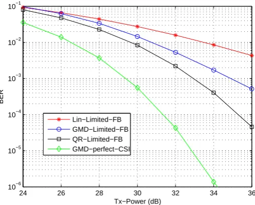
3.9 BER versus Tx-Power with limited feedback (8 feedback bits per block, and 32 bits transmitted per block). . . 56

3.10 BER versus Tx-Power with limited feedback (8 feedback bits per block, and 24 bits transmitted per block). . . 56

(13)

3.12 Comparing four transceivers for 100 channel realizations, with each antenna power

≤9. The x-axis represents the total power constraint. . . 63

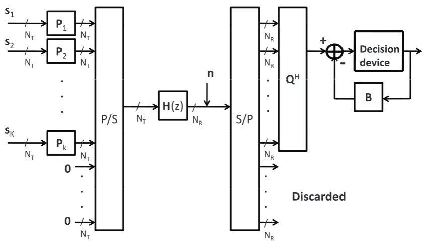
4.1 The ZP-BD-GMD transceiver. The signal vectorsiis first linear precoded by the

uni-tary matrixPi. The precoded symbol vectors andNP zero vectors are then passed

through a parallel-to-serial converter before transmitting to channelH(z). The re-ceiver discards the contaminated signals, and passes the clean signal through DFE.

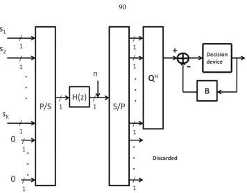
QH is the feedforward filter, andBis the feedback filter, whose coefficients are ob-tained from the entries inL. . . 76 4.2 The ZP-BD-GMD transceiver for SISO channels. The lazy precoder is used. The vector

with signal symbolssiappended withNPzeros is passed through a parallel-to-serial

converter before transmitting to the channelH(z). The receiver discards the contam-inated signal, and passes the clean signal through DFE.QH_{is the feedforward filter,}

andBis the feedback filter. . . 90 4.3 The effective channel gain of ZF-BD-GMD and ZF-Optimal transceivers for channel

Ha(z). . . 92

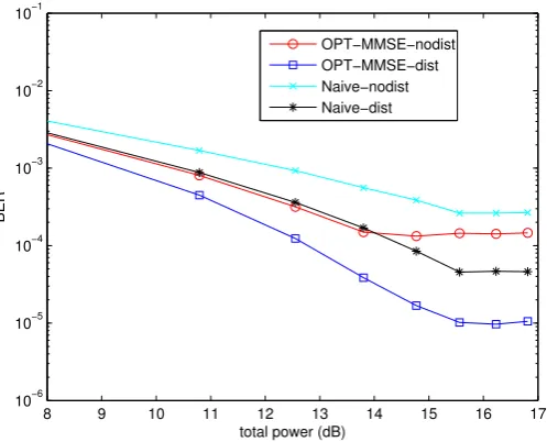
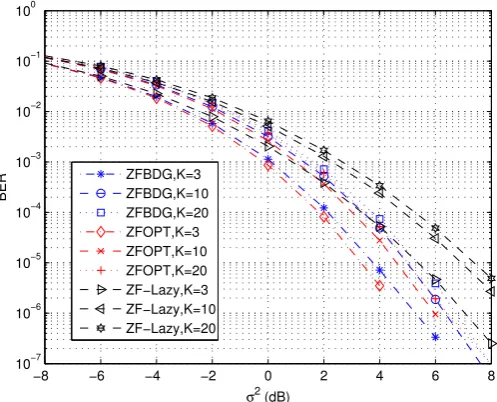
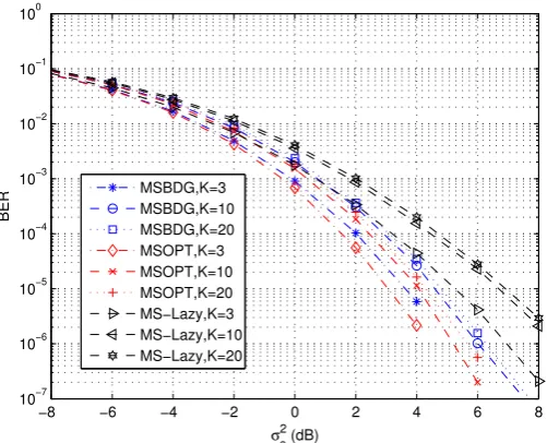
4.4 The BER performance of the zero-forcing systems for MIMO (NT =NR= 2) Rayleigh

channels of order3, withK = 3,K = 10, andK = 20. “ZFBDG” represents the ZF-BD-GMD system; “ZFOPT” represents the ZF-Optimal system; and “ZF-Lazy” repre-sents the lazy precoder with zero-forcing DFE. . . 93 4.5 The BER performance of the MMSE systems for MIMO (NT = NR = 2) Rayleigh

channels of order3, withK = 3, K = 10, andK = 20. “MSBDG” represents the MMSE-BD-GMD system; “MSOPT” represents the MMSE-Optimal system; and “MS-Lazy” represents the lazy precoder with MMSE-DFE. . . 94 4.6 The BER performance of the zero-forcing systems for SISO (NT =NR = 1) Rayleigh

channels of order 3, with K = 3, K = 10, and K = 20. “ZFOPT” represents the ZF-Optimal system; and “ZF-Lazy” represents the lazy precoder with zero-forcing DFE. 94 4.7 The BER performance of the MMSE systems for SISO (NT =NR= 1) Rayleigh

chan-nels of order3, withK = 3,K = 10, andK = 20. “MSOPT” represents the MMSE-Optimal system; and “MS-Lazy” represents the lazy precoder with MMSE-DFE. . . . 95

(14)

5.2 A direct implementation of the PLT. . . 106

5.3 The PLT implemented using MINLAB(I) structure. . . 106

5.4 The GTD transform coder implemented using MINLAB(I) structure. . . 108

5.5 The BID Transform coder implemented using MINLAB(I) structure. . . 111

5.6 Use of GTD-TC in the progressive transmission context. . . 111

5.7 Performance of different transform coders with optimal bit allocation. Input covari-ance matrix has a high condition number (107_). _{. . . 115}

5.8 Performance of different transform coders with optimal bit allocation. Input covari-ance matrix has a low condition number (103). . . 115

5.9 Comparison of coding gain of different transform coders with optimal bit allocation. Input covariance matrix has a high condition number (107_{). . . 116}

5.10 Performance of different transform coders with uniform bit allocation. Input covari-ance matrix has a high condition number (107_{). . . 116}

5.11 Performance of different transform coders with uniform bit allocation. Input covari-ance matrix has a low condition number (103_{). . . 117}

5.12 Subtractive dithered GMD transform coder. . . 120

5.13 Nonsubtractive dithered GMD transform coder. . . 120

5.14 The equivalent model of dithered GMD transform coder. . . 122

5.15 Performance of different transform coders. . . 124

6.1 The biorthogonal GTD subband coders forM = 4. . . 129

6.2 A restricted case of the biorthogonal GTD subband coders forM = 4. . . 140

6.3 Coding gain of subband coders withM = 3for the AR(1) process withρfrom0.85to 0.95. . . 142

6.4 Coding gain of subband coders withM = 4for the AR(2) process withρfrom0.95to 0.99andθ=π/3. . . 143

6.5 Monotone behavior of the coding gain as a function of the number of channels for the AR(1) process withρ= 0.95. . . 144

6.6 Nonmonotone behavior of the coding gain as a function of the number of channels for the AR(2) process withρ= 0.975andθ=π/3. . . 144

(15)

(16)

List of Tables

5.1 Design and Implementation Costs of Transform Coders . . . 111

(17)

Chapter 1

Introduction

Signal processing is an art that deals with the representation, transformation, and manipulation of signals and the information they contain based on their specific features. It is a technology that spans an immense set of disciplines. The field of signal processing has always benefited from the interaction between theory, applications, and technologies for implementing the systems. The de-velopment of signal processing theory, in particular, relies heavily on mathematical tools including analysis, probability theory, matrix theory, and many others. The theory of majorization, which is an extremely useful tool for deriving inequalities, was recently introduced to signal processing so-ciety. This also led researchers to develop a fundamental matrix decomposition called generalized triangular decomposition (GTD), which was shown to be general enough to include many existing orthogonal matrix decompositions as special cases.

The present thesis is a contribution towards the use of these newly developed mathematical tools in several important signal processing problems. In particular, we focus on the signal pro-cessing for communications and filter bank designs. With these powerful mathematical tools at hand, we revisit some classical problems and show that the theories of majorization and GTD pro-vide a general framework for solving these problems. For some important new problems, these new tools also provide elegant solutions.

(18)

Chapter 9 of [111].

1.1

MIMO Transceiver Optimization

1.1.1

MIMO Channel Models

The first part of this thesis focuses on the communication system design, in particular, transceiver design for multiple-input multiple-output (MIMO) channels. We consider modeling the communi-cation channels as linear time invariant (LTI) systems with additive noise. The focus is on MIMO channel models because they represent a unified way to model a wide variety of many different types of communication scenarios. Also, the matrix-vector notation can be conveniently used to handled MIMO channel models. This fact is crucial for applying elegant matrix theory results to many communication system design problems.

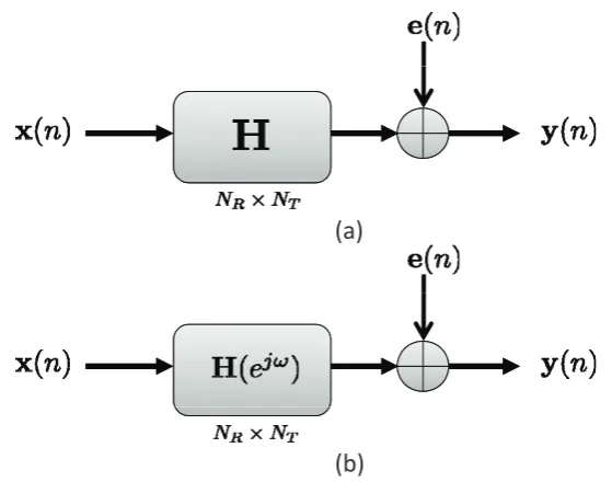
The models we considered are the MIMO frequency flat channel model, and the MIMO fre-quency selective channel model, which are shown in Fig. 1.1(a) and Fig. 1.1(b), respectively. Here

x(n)is theNT ×1transmitted signal,y(n)is theNR×1received signal, ande(n)is theNR×1

additive noise introduced by the channel. TheNR×NT channel matrix is modeled asH(ejω)for

the frequency selective case. When the channel is memoryless, the channel is modeled as the con-stant matrixH. In these linear models, the received signal is the channel noise plus the transmitted signal after being linearly distorted by the channel. For frequency flat channels, the input/output relation of the system is

y(n) =Hx(n) +e(n),∀ integern.

For frequency selective channels, the received signaly(n)is the noisee(n)plus the output of the filterH(ejω₎_{in response to}_x₍_n₎_{. The MIMO channel models are general enough to model many}

different communication scenarios, as we will see from several examples in the following.

(19)

(a)

[image:19.595.186.466.104.324.2]

(b)

Figure 1.1: (a) Frequency flat MIMO channel model. (b) Frequency selective MIMO channel model.

wireless systems. If spatial diversity is simultaneously exploited at both the transmitter and the receiver, it is natural to use a MIMO representation. In this setting,NRis the number of

receiving antennas, andNT is the number of transmitting antennas.

2. Blocked scalar channels with finite memory: The scalar channels with memory can be converted to MIMO channels without memory in a number of ways. Two of the most common tech-niques for this are the zero-padding and cyclic-prefix precoding techniques [89]. The zero-padding precoding produces the effective frequency flat channel matrixH having Toeplitz structure, and the cyclic-prefix precoding produces circulant matrix H. The elements of H

in each case can be obtained from the time domain samples of the channel coefficients. The cyclic-prefix precoding is in particular of great interests since it leads to OFDM and DMT systems, which have great performance advantages in wireless communication systems and digital subscriber line (DSL) systems.

In addition to the two examples mentioned above, there are many other common communica-tion scenarios that can be modeled appropriately as MIMO channel models. These include multi-carrier systems on frequency selective channels, systems exploiting polarization diversity, and code division multiple access (CDMA) channels. Note that the structures ofHandH(ejω₎_depend

(20)

opti-mization problem with any givenHorH(ejω)

1.1.2

Transceiver Optimization and History

Transceiver optimization has had a long history since the 1950s. Because of the technological break-through of DSL, MIMO, and wireless communications, research in this area has become very in-tense since the 1990s. However, much of the recent work has its roots in the mathematical meth-ods and signal models in earlier papers. This is the reason why we shall review the history of transceiver optimization in somewhat detailed fashion. The readers interested in more compre-hensive treatments are referred to Chapter 9 in [111].

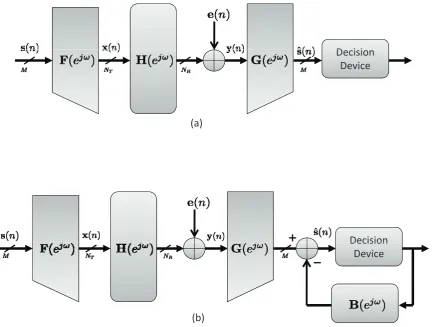
Fig. 1.2 shows the transceiver models we consider in this thesis. The channelH(ejω₎_(frequency

selective in general) is assumed to be with dimensionNR×NT, ande(n)is the additive channel

noise. Heres(n)is theM ×1symbols,x(n)is the transmitted signal,y(n)is the received signal, andˆs(n)is the input to the scalar decision devices. Fig. 1.2(a) shows the linear transceiver with precoderF(ejω₎_{, and equalizer}_G₍_ejω₎_{. Fig. 1.2(b) shows the DFE transceiver with precoder}_F₍_ejω₎_,

feedforward filterG(ejω₎_{, and feedback filter}_B₍_ejω₎_{. Note that the successive decision feedback}

and decoding is performed at the receiver. The matrixB(ejω)is therefore restricted to be strictly upper triangular for casual implementation. In both systems, the transmitted signalx(n)is the symbols(n)after linearly precoded byF(ejω₎_{, and the received signal}_y₍_n₎_{is formed by channel}

noisee(n)plus the transmitted signal distorted by the channelH(ejω₎_{. Also note that the model in}

Fig. 1.2 is general enough to model the frequency flat case. If the channel is frequency flat, where the channel is a constant matrixH, then all the other matrices in Fig. 1.2 are also constant matrices. The transceiver optimization problem is to optimize{F(ejω₎_,_G₍_ejω₎_}_{for the linear transceiver,}

or{F(ejω₎_,_G₍_ejω₎_,_B₍_ejω₎_}_{for the DFE transceiver, subject to appropriate constraints under some}

assumptions of the channel state information available, such that some measure of performance is optimized. This simple model leads to a multitude of interesting optimization problems depending upon the applications. For example, one may wish to minimize the bit error rate under a total average power constraint or individual antenna power constraints. One may also consider the quality of service problem to minimize the transmitted power under some bit rate and bit error rate constraints for subchannels.

(21)

assump-D

i i

Decision

Device

(a)

Decision

Device

[image:21.595.111.544.215.542.2]

(b)

Figure 1.2: (a) The general form of linear transceivers with channelH(ejω₎_{, precoder}_F₍_ejω₎_{, and}

equalizerG(ejω₎_{. (b) The general form of DFE transceivers with channel}_H₍_ejω₎_{, precoder}_F₍_ejω₎_,

(22)

tions on the channel state information (CSI). CSI at the receiver (CSIR) is traditionally obtained via the transmission of pilot symbols that allows the estimation of the channel. CSI at the transmitter (CSIT), on the other hand, cannot be directly obtained as such. One scheme to obtain CSIT is to send the transmitter the quantized version of channel coefficients once the receiver estimates the chan-nel. Another popular scheme is the so-calledlimited feedbacktechnique, in which the receiver feeds back the index of the precoder in the predetermined codebook to inform the transmitter which pre-coding scheme to use. Although the CSIT may not be perfect in practice, it is still crucial to discuss theoretically how to jointly optimize the transmitter and receiver assuming perfect CSIT and CSIR are both at hand. This serves as a performance upper bound and gives insight to practical designs. At the same time, it is also important to consider the more robust designs, i.e., the situation where perfect CSIT and/or CSIR is not available.

The history of linear transceiver optimization (also see Chapter 9 of [111] for more detailed review) can be dated back to the paper by Costas [16] in 1952, in which for the identity continu-ous channel the author addressed the problem of optimizingprefilterandpostfilterto minimize the mean square error of the reconstructed signal. It was shown that the optimal scheme is of the form that adopts some Wiener-type receiver and some power loading on the transmitted signal across frequency. Optimization of the transceivers for discrete symbol streams under channel distortions was then considered by Berger and Tufs [6]. The Wiener-type receiver was again shown to be opti-mal, and the transmission scheme is similar to the fashion of Costas but with some modifications. In 1971, Chan and Donaldson [11] extended the optimization to cover sampling and quantization as in digital communication systems. The design of filters for the case of bandlimited channels was later addressed by Chevillat and Ungerboeck [13].

Another line of research is on replacing the linear receiver by the decision feedback equal-izer (DFE) to combat the inter-symbol interference (ISI). In general, DFEs are superior to linear equalizers—slight for good channels, moderate for channels with severe attenuation distortion, and substantial for channels with spectral nulls. Price [84] assumed a zero-forcing condition and found the joint optimum DFE receiver and linear transmitter. The joint MMSE transmitter and receiver were later obtained by Salz [87]. Several other authors of important papers on DFE transceiver optimizations include Falconer and Foschini [22], Messerschmitt [66], and Witsenhausen [118].

(23)

square MIMO filtersfor the case of transmitting a discrete time sequence through a continuous time channel under the average power constraint. Salz showed that the optimal equalizer was identified to be a Wiener-type filter and the transmitter was obtained from the Karush-Kuhn-Tucker (KKT) condition for constrained optimization. By using a theorem based on the concept of Schur-convexity provided by Witsenhausen, Salz showed that the optimal solution can be obtained by diagonalizing the channel using singular value decomposition (SVD), and deriving the optimal filters for the diagonal channel. This diagonalization was later to be observed ubiquitously in various MIMO transceiver optimization problems. In 1988 Malvar and Staelin [63] addressed the transceiver optimization for rectangular channel and transceiver matrices. Instead of total power constraints, individual antenna power constraints are also considered in [45] and [63]. Besides linear transceivers, the MIMO DFE transceiver optimization was addressed by Yang and Roy in [138], in which the authors proposed the optimal system that minimizes the MSE simultaneously minimizes the geometric MSE.

In 2003 Palomaret al.[73] officially introduced the theory of majorization and Schur-convexity to the linear transceiver optimization, and thus unified many existing works in the literature. In this milestone paper, the authors proposed a formulation that covers a wide range of objective func-tions and constraints for MIMO transceiver optimization problems. The solufunc-tions can be divided into different classes depending upon whether the objective function is convex or Schur-concave. If the objective function is Schur-concave in the mean square errors of the subchannels, the diagonalizing structure is always optimal. If the objective is Schur-convex, the optimal solution diagonalizes the channel after a very specific rotation of the transmitted symbols. Many of the ex-isting works were shown to be special cases within this framework. Since this paper, the theory of majorization and convex optimization became more heavily used in this field.

(24)

published by Zhang et al. [142], and Xuet al. [137]. A unified framework for DFE transceivers under total average power constraints, which can be seen as a parallel counterpart of Palomar et al.’s 2003 linear transceiver paper, was also reported in [41], and independently in [90]. Based on the concept of multiplicative majorization, the framework covers a wide range of objective func-tions and the solufunc-tions are divided into different classes depending upon whether the objective function is Schur-convex and Schur-concave in the logarithms of the MSEs in the subchannels. The UCD scheme was shown to be optimal for the class of Schur-convex functions. For the class of Schur-concave functions, the optimal solution becomes the degenerate linear transceiver.

It is sometimes desirable to optimize the transceiver system with specific quality of service (QoS) for each of the subbands, which could be assigned to different users. Pandharipande and Dasgupta [18] extended the work of [50] and used majorization theory to established some results for digital multitone (DMT) systems. In 2004, Palomaret al. extended their 2003 milestone paper and considered the QoS problem [77] for linear transceivers. Jiang et al. on the other hand consid-ered the QoS problem for DFE transceivers and proposed the so-calledtunable channel decomposition

(TCD) [39]. This later led them to the discovery of generalized triangular decomposition (GTD) [38]. Most of the results described above assume the channel, precoder, and equalizer to be constant matrices. For frequency selective channels, some of the early papers considered frequency de-pendent precoder and equalizers. The solution ended up being ideal unrealizable filters [88, 138]. These papers still have great value since they provide a theoretical upper bound and give insight to design practical systems. More recently some researchers considered the transceivers with finite memory and showed how to design these filters for practical applications. For example, Mertins [67] constrained the precoder to be a FIR matrix but the receiver can in general to be IIR. The work of Phoong et al. [81] restrained both the precoder and equalizer to be FIR filters. The paper by Vijaya Krishna and Hari [113] considered the optimization of minimum redundancy precoders, which was originally proposed by Lin and Phoong [80].

(25)

transceivers for many different communication scenarios. This framework was later extended to the DFE transceivers in [91], and Grassmannian codebook was again found to be useful.

Such is the very brief history of transceiver optimization. Researchers across many decades have devoted themselves to this field. As mentioned above, the 2003 paper by Palomaret al. officially brought the theory of majorization and Schur-convexity into this field and changed the way people view these problems. By considering the DFE transceiver counter part, Jianget al. discovered a novel matrix decomposition—generalized triangular decomposition (GTD) that was shown to be useful in the MIMO transceiver QoS problem. This thesis continues this line, and further shows that the theory of majorization and GTD is useful not only in the scenarios described in these earlier papers, but also in broader signal processing applications including other important transceiver optimization problems, transform coding problems, and filter bank optimization.

1.2

Transform Coder and Signal Adapted Filter Bank

Optimiza-tion

A filter bank (FB) is used to decompose a signal into several bands, which are then processed in-dependently and combined. Processing resources can be allocated according to specific features in each of the subbands. The optimization of filter banks based on knowledge of input statistics has been of great interest in signal processing for a long time. The transform coder optimization, before the time of the filter bank, was first considered by Huang and Schultheiss [33] in the 1960s. Since then, there have been many advances in the theory of filter banks, wavelets, and their ubiq-uitous signal processing applications including data compressions, signal denoising, and digital communications.

Fig. 1.3 shows the standardM-channel filter banks which can be found in many signal process-ing books, e.g., [107]. The subband processorsPican represent many kinds of linear or nonlinear

(26)

such that the polyphase matricesR(ejω)andE(ejω)satisfy

R(ejω)E(ejω) =I

for allω. This is also called the perfect reconstruction (PR) property. The reason is that in the absence of any subband processing, the PR property impliesxˆ(n) = x(n)for alln. For the special case where the polyphase matrixE(ejω₎_{is paraunitary (i.e., unitary for all}_ω_{) and}_R₍_ejω_{) =}_E†₍_ejω₎_,

the filter bank is called anorthonormal filter bank. In this case, the set ofM filters{Hk(ejω)}is said

to be orthonormal, and the set of synthesis filters can be shown to beFk(ejω) =Hk∗(e jω₎_.

A filter bank whose filters depend on knowledge of the input statistics is called a signal-adapted filter bank. The subband coding problem, which is an instance of the signal-adapted filter bank design problems, is to quantize the subband signals rather than to quantize the original signal directly, based on the knowledge of input statistics. While other performance measures in the rate-distortion sense are possible, one measure that receives much attention is thetheoretical coding gain. The coding gain maximization problem is equivalent to the minimization of the average mean-square error of the reconstructed quantized signal by designing the filter bank and the bit allocation scheme.

M

!"

M

!"

M

Analysis

Bank

M

!"

M

Subband

processors

Synthesis

Bank

Figure 1.3: TheM-channel maximally decimated filter bank with uniform decimation ratioM.

(27)

M

!"M

1

M

!"M

z

1

z

1

z

1

z

Polyphase

matrix

M

!"M

Subband

processors

Polyphase

matrix

z

1

z

Figure 1.4: The polyphase representation of theM-channel maximally decimated filter bank.

if and only if theM-fold blocked versionx(n)is wide sense stationary (WSS), meaning that the mean and autocorrelation ofx(n)do not depend onn. In this thesis, we will adopt this assump-tion and also assume thatx(n)and hencex(n)are zero mean. In addition, we will assume that we only have knowledge of the second order statistics ofx(n), namely the autocorrelation function

Rxx(k) =E[x(n)x†(n−k)]. The power spectral density (psd) matrixSxx(ejω), which is simply the

Fourier transform ofRxx(k), will often appear in the discussion.

We now give a brief overview of the past work in this field. For the special case where the matricesE(ejω₎_and_R₍_ejω₎_{are constant, the system in Fig. 1.4 is said to be a}_{transform coder}_{. In}

(28)

theprincipal component filter banks(PCFB) was introduced and developed in [100]. Theoretical re-sults for the optimality of an orthonormal filter bank with unconstrained filter order was developed by Vaidyanathan in [106]. It was shown that there are two necessary and sufficient conditions for the optimal orthonormal subband coder, namely,total decorrelationandspectrum majorization. For the case of biorthogonal filter banks, it was conjectured by Vaidyanathan and Kirac that the op-timal structure is the cascade of the opop-timal orthonormal filter bank, and a set of half-whitening filters applied to the signal in each individual subband [109]. This conjecture was later proven to be true by Moulinet al. in [70]. The authors in [70] also showed the two fundamental properties, total decorrelation and spectrum majorization, are also two necessary conditions for optimality of biorthogonal filter banks. The same group of researchers also extended their work and derived the optimal subband coders when there is no perfect reconstruction constraint [68].

These theoretical results provide a nice performance bound on the filter banks with uncon-strained filter order. However, finite length filter implementation methods are needed for practice. The finite impulse response (FIR) solutions to the orthonormal and biorthogonal filter banks are also discussed extensively in the literature [44, 58, 69, 70, 97, 98, 102].

As mentioned earlier, principal component filter bank (PCFB) is a closely related concept. PCFB was shown to be simultaneously optimal for a variety of objective functions within the class of orthonormal filter banks. By definition, a PCFB for an input psdSxx(ejω)and for a classCof filter banks, if it exists, is one whose subband variance vector

σ= [σ2_v₀σ_v2₁ · · · σ_v2_M₋₁]T

(29)

upper bound on the performance we can expect from paraunitary filter banks.

Such is the very brief review of the filter bank optimization problem. The research in this field, since as early as Huang and Schultheiss’ transform coding paper, has been continued for almost five decades. In this thesis, we introduce the generalized triangular decomposition (GTD), which was originally developed in the MIMO communication society, to this field. We will show that the concept of GTD and the theory of multiplicative majorization give this classical problem a completely new look. Many novel coder structures are proposed, and several theoretical results are established. The connection of the GTD filter bank to the PCFB will also be indicated.

1.3

Outline and Scope of the Thesis

There are two major signal processing problems considered in detail in this thesis. The first prob-lem of focus is transceiver designs for MIMO communications (Chapter 3, 4). We consider many different MIMO communication scenarios, including the optimization of DFE transceivers when bit allocation is allowed, QoS problem for DFE transceivers, transceiver design under individual antenna power constraints, and also the transceiver design for frequency selective channels. Based on the concept of majorization and the use of generalized triangular decomposition, many novel designs are proposed, and performance analyses are provided. The second problem of focus is the data compression and signal-adapted filter bank optimization (Chapter 5, 6). We first revisit the classical transform coding problem. Then, based on GTD, we propose and optimize a new sub-band coding structure, which can be shown to have superior performance than the existing ones. Many theoretical results as well as practical concerns will be presented. The connection between the current thesis and existing work in literature will also be clearly indicated. In the following we briefly discuss the scope of each chapter.

1.3.1

Review of Majorization, Matrix Theory, and Generalized Triangular

De-composition (Chapter 2)

(30)

majorization is introduced as well.

Then, we review the connections between majorization and the matrix theory. Additive ma-jorization is closely related to the properties of diagonal elements and eigenvalues of Hermitian matrices. On the other hand, multiplicative majorization is the complete characterization of the relation between singular values and eigenvalues of complex-valued square matrices. We then introduce the generalized triangular decomposition (GTD) developed by Jianget al.. This decom-position is very fundamental and incorporates many existing well-known matrix orthogonal de-compositions as special cases. Several examples of the GTD will be discussed in this chapter as well. Finally, we will review some mathematical properties of the block diagonal geometric mean decomposition (BD-GMD).

1.3.2

Transceiver Designs for MIMO Frequency Flat Channels (Chapter 3)

In Chapter 3, we consider several transceiver design problems for frequency flat MIMO channels using GTD and majorization theory. Mainly two scenarios are considered in detail.

The first part of this chapter considers the joint optimization of MIMO transceivers with linear precoders, decision feedback equalizers (DFEs), and bit allocation schemes. It is shown that the generalized triangular decomposition (GTD) offers an optimal family of solutions. The optimal linear transceiver (which has a linear equalizer rather than a DFE) with optimal bit allocation, as well as the DFE transceiver using the geometric mean decomposition (GMD), are members of this family. The QR-based system used in the VBLAST system is yet another member of the optimal family and is particularly well suited when limited feedback is allowed from receiver to transmit-ter. Thus, GTD provides a general theoretical framework for this optimization problem, and gives insight on the practical designs.

(31)

to also incorporate any finite number of linear constraints to the covariance matrix of the input.

1.3.3

Transceiver Designs for MIMO Frequency Selective Channels (Chapter

4)

While the previous chapter focuses on frequency flat MIMO channels, this chapter is devoted to transceiver designs for MIMO frequency selective channels. We consider using the block-diagonal GMD (BD-GMD), a novel matrix decomposition that was originally proposed by Linet al. in 2008 [47] for MIMO broadcast channel, to design the DFE transceivers. Two new BD-GMD transceivers are proposed: the ZF-BD-GMD system, where the receiver is a zero-forcing DFE (ZF-DFE), and the MMSE-BD-GMD system, where the receiver is a minimum-mean-square-error DFE (MMSE-DFE). We show that the BD-GMD systems have many optimal properties and at the same time computationally efficient. These make the proposed BD-GMD favorable designs for frequency selective MIMO channels.

1.3.4

The Role of GTD in Transform Coding (Chapter 5)

In this chapter we revisit the classical transform coding problem from the view point of GTD and majorization theory. In the first part of this chapter, a general family of optimal transform coders (TC) is introduced based on GTD. This family includes the Karhunen-Lo´eve transform (KLT), and the generalized version of the prediction-based lower triangular transform (PLT) introduced by Phoong and Lin in 2000 [79], as special cases. The coding gain of the entire family, with optimal bit allocation, is equal to those of the KLT and the PLT. Other special cases of the GTD-TC are the GMD (geometric mean decomposition) and the BID (bidiagonal transform). The GMD in particu-lar has the property that the optimum bit allocation is a uniform allocation; this is because all its transform domain coefficients have the same variance, implying thereby that the dynamic ranges of the coefficients to be quantized are identical.

(32)

dithered (GMD-NSD) transform coder where the decoder has no knowledge about the dither. Un-der the uniform bit loading scheme, it is shown that the proposed dithered GMD transform coUn-ders perform significantly better than the original GMD coder in the low rate regime.

1.3.5

The Role of GTD in Filter Bank Optimization (Chapter 6)

In this chapter we consider the filter bank optimization based on the knowledge of input signal statistics. GTD and the theory of majorization is again used to give a new look to this classical problem. We propose the GTD filter bank as a subband coder for optimizing the theoretical coding gain. The focus is on perfect reconstruction orthonormal GTD filter banks and biorthognal GTD filter banks. In both cases, we show that there are two fundamental properties in the optimal solutions, namely,total decorrelationandspectrum equalization. The optimal solutions can be obtained by performing the frequency dependent GTD on the Cholesky factor of the input power spectrum density matrices. We also show that in both theory and numerical simulations, the optimal GTD subband coders have superior performance to optimal traditional subband coders. In addition, the uniform bit loading scheme, with no loss of optimality, can be used in the optimal biorthogonal GTD coders. This solves the granularity problem in the conventional optimum bit loading formula. The proposed GTD filter banks can also be used in MIMO communication systems. We consider the transceiver with linear precoding and zero-forcing decision feedback equalization for MMO frequency selective channels. The quality of service (QoS) problem of minimizing the transmitted power subject to the bit error rate and total bit rate constraints is considered. Optimal systems with orthonormal precoder and unconstrained precoder are both derived and shown to be related to the frequency dependent GTD of the channel frequency response.

1.4

Notations

The notations used throughout this thesis are defined as follows. Boldfaced lower case letters rep-resent column vectors. Boldfaced upper case letters and calligraphic upper case letters are reserved for matrices. Superscripts∗_{, and}T_{, as in}_a∗_,_AT _{denote the conjugate and the transpose,}

(33)

the notation diag(x)denotes the diagonal matrix with diagonal terms equal to the elements inx. In figures, “↑ N” and “↓ N” denote the signal upsampler and downsampler, respectively [107]. For any x ∈ Rn_, _x

[1] ≥ x[2] ≥ · · · ≥ x[n] denote the elements of x in descending order, and x(1) ≤ x(2) ≤ · · · ≤ x(n)denote the elements ofxin ascending order. For two real vectorsxand

y,x+ yory≺+ xdenotes thatxadditively majorizesy[65]. For two complex vectorsxandy,

(34)

Chapter 2

Review of Majorization, Matrix

Theory, and Generalized Triangular

Decomposition

In this chapter we will give a brief overview of the necessary mathematical preliminaries, on which many of the results in this thesis are based. We will first introduce majorization theory, Schur-convexity, and the relation to matrix theory. Then, we will review the generalized triangular de-composition (GTD). A special case of GTD, namely the block-diagonal geometric mean decompo-sition (BD-GMD), will also be introduced.

2.1

Review of Majorization and Schur Convexity

The idea of majorization and Schur-convexity is very fundamental to many problems in linear alge-bra and optimization. One of the earliest references on this topic is the book by Hardy, Littlewood, and P ´olya [29]. More recent references include Marshall and Olkin [65]. The relation between ma-jorization theory and matrix theory is discussed extensively in [32]. Many of the results reviewed in this chapter are used in the thesis. The readers interested in more comprehensive treatments are also referred to [111].

2.1.1

Additive Majorization and Schur Convexity

(35)

The notion of majorization makes this precise.

Definition 2.1:(Additive Majorization.) For anyx,y∈Rn_{, the vector}_x_{is said to additively}

majorizey(oryis additively majorized byx), and is denoted asx+yif and only if1

k

X

i=1

x[i]≥

k

X

i=1

y[i], ∀k= 1,2,· · ·, n−1

and

n

X

i=1

x[i]=

n

X

i=1

y[i]

From the above definition it can be seen that the notion of majorization is invariant to any permutation of the elements in the vector, i.e.,

x+yif and only ifΠ1x+ Π2y

for any permutation matrixΠ1andΠ2. The ordering “+” defined onRn is apreorderingbut not

partial ordering(see p.13 of [65]). However it is also partial proper orderingif it is regarded as an ordering of sets of numbers rather than as an ordering of vectors. It it important to remember that two sequences may not have any majorization relationship.

One simple observation is that the vector of the arithmetic mean of the elements is always additively majorized, which is shown in the following example.

Example 2.1:Letx∈Rn_{, and}_x_{denote the constant vector with the value equal to the arithmetic}

mean of the elements inx, i.e., 1

n

Pn

i=1xi. Then,x+x. ♦

The notion of majorization is closely related to Schur-convexity. Specifically, Schur-convexity characterizes the differentiable functions that preserve the ordering+onRn(see p.53 of [65]).

Definition 2.2:(Schur-Convexity.) A real-valued functionφdefined on a setA⊆Rn_{is said to be}

Schur-convex onAif

x≺+yonA ⇒φ(x)≤φ(y). 1_{The notation}_x

(36)

In addition,φis said to be Schur-concave if and only if−φis Schur-convex.

Note that the sets of Schur-concave and Schur-convex functions do not form a partition of the set of all functions. This fact will be illustrated later in Fig. 2.1.

There are many beautiful examples of Schur-convex/concave functions that arise in optimiza-tion problems in signal processing and communicaoptimiza-tions. Some of the examples follow from the theorems presented in this section. The first theorem shows the relation between convex functions and Schur-convex functions [29, 65].

Theorem 2.1.1 The inequality

n

X

i=1

g(xi)≥ n

X

i=1 g(yi)

holds for all continuous convex functions g : R → R if and only if x + y. Therefore, the function f(x) =Pn

i=1g(xi)is a Schur-convex function inx. ♦

Example 2.2: (Log-Product.) Letg(x) = log(x)for any positivexand thusg is convex. The function

f(x) =

N

X

i=1 g(x) =

N

X

i=1

log(x) = log

N

Y

i=1 xi

!

is Schur-convex. ♦

Example 2.3:(The average probability of error of MIMO communication systems.) The average sym-bol error probability of a scalar Gaussian communication channel is given by (see p.383 - p.385 of [111])

Pe(y) =cQ(A/

√

y),

wherecandAare constants depending on the constellations (the size of PAM or QAM signaling) used and the signal power,yis the error variance, andQ(·)is theQ-function. It was shown that Q(A/√y)is convex iny for y < A2/3. Therefore, the average symbol error probability of a M-channel MIMO communication system is given by

Pe(y) =

c M

M

X

k=1 Q(√A

yk

(37)

Using Thm. 2.1.1, it can be shown thatPe(y)is Schur-convex ifyk < A2/3for allk. ♦

There are a number of simple but useful facts relating to compositions that involve Schur-convex and Schur-concave functions (p.61 of [65]). Ifg(x)is Schur-convex thenf(x) = h(g(x))is Schur-convex, as long ash(·)is a non-decreasing real function of its argument. More relations are shown as follows:

g(x)is Schur-convex andh(y)is non-decreasing⇒f(x)is Schur-convex; g(x)is Schur-convex andh(y)is non-increasing⇒f(x)is Schur-concave; g(x)is Schur-concave andh(y)is non-decreasing⇒f(x)is Schur-concave;

g(x)is Schur-concave andh(y)is non-increasing⇒f(x)is Schur-convex.

2.1.2

Multiplicative Majorization

The notion parallel to additive majorization ismultiplicative majorization, which finds application in various signal processing problems [133, 28, 38].

Definition 2.3:: (Multiplicative Majorization[65, 38].) For anyx,y∈Rn₊, the vectorxis said to multiplicatively majorizey(denoted asx×y) if and only if

k

Y

i=1

x[i]≥

k

Y

i=1

y[i], ∀k= 1,2,· · · , n−1

and

n

Y

i=1

x[i]=

n

Y

i=1

y[i].

From these two definitions, we observe that if all elements ofxandyare positive, then

x×y⇐⇒ln(x)+ln(y)

(38)

Figure 2.1: The illustration of the relations between sets of functions [41].

Example 2.3: Letx ∈Rn

+ andˆxdenotes the constant vector with the value equals to the geo-metric mean of the elements inx, i.e. pQn n

i=1xi. Then

x×ˆx.

♦

A type of function closely related to the notion of multiplicative majorization is the composition of Schur-convex functions and the exponential function. The compositionf ◦exp : RN _→ _R_is

defined as

f◦exp(x)≡f(ex1_{, e}x2_,_{· · ·}_{, e}xN₎_.

The following theorem is a direct consequence of the composition rule of Schur-convex func-tions with increasing convex funcfunc-tions.

Theorem 2.1.2 (a) The composite functionf◦expis Schur-convex if functionf :R⊆Rnis Schur-convex. (b) If the composite functionf ◦expis Schur-concave, thenf :R⊆Rnis Schur-concave. ♦

(39)

2.2

Relation to Matrix Theory

There are several important facts connecting matrix theory and the notion of majorization. These beautiful results in the matrix singular values and eigenvalues of a square matrix, or eigenvalues and diagonal terms of a Hermitian matrix, serve as the foundation of the results established in this thesis.

2.2.1

Hermitian Matrices

The first result we present here was proved by Schur in 1923. It relates the diagonal elements of a Hermitian matrix to its eigenvalues [65].

Theorem 2.2.1 (Diagonal elements and eigenvalues of a Hermitian matrix [31, 65].) LetRbe ann×n

Hermitian matrix with diagonal elements denoted by the vectordand eigenvalues denoted byλ. Then

λ+d. (2.1)

That is, for a Hermitian matrix, the vector of eigenvalues majorizes the vector of diagonal elements. ♦

For Theorem 2.2.1, the converse is also true. Therefore, the notion of additive majorization is the strongest relation we can have between the diagonal elements and the eigenvalues of Hermitian matrices.

Theorem 2.2.2 (Existence of a particular Hermitian matrix, see Thm 4.3.32 in [31].) Letλ,d∈Rn_{, and}

satisfy (2.1), then there exists a Hermitian matrixMsuch thatdis the vector of diagonal elements ofM,

andλis the vector of eigenvalues ofM.

The above two theorems are very important in the optimization of transceivers for MIMO chan-nels. One nice application is Witsenhausen’s observation used in [88]. The other use of these two theorems is in the unified framework of linear transceiver optimization provided by Palomaret. al

in [73]. The following example is very crucial in establishing the results of [73].

Example 2.4:Letd,λ∈Rn_{denote the vector of diagonal elements and the vector of eigenvalues}

of a Hermitian matrixM, respectively. Letd¯ = ¯d×[1,1,· · · ,1]T _{denote the vector with all elements}

(40)

elements isd¯. Here is a way to obtain such matrix. Suppose the eigenvalue decomposition ofM

isM = TΛT†. LetQ be any unitary matrix with identical magnitudes for all its elements, i.e.,

|[Q]ij| = 1/

√

n.Examples of such matrices are the normalized DFT matrix and the normalized Hadamard matrix for certain values ofn[49, 73]. LetM0 =Q†T†ΛTQ, then for any diagonal of

M0,

[M0]kk= n

X

i=1

[Q†]kiλi[Q†]ik=

1

n

X

i=1 λi= ¯d.

Therefore,M0is an example of a Hermitian matrix with diagonal elementsd¯and eigenvaluesλ.♦

2.2.2

Complex-Valued Square Matrices

The fundamental results on the relation between eigenvalues and singular values of a square complex-valued matrix was first established by Weyl in 1949 [134]. The findings can be presented as follows:

Theorem 2.2.3 (Eigenvalues and singular values [134, 32, 140].) LetM∈Cn×n_{, and let}_λ

iandσidenote

the eigenvalues and singular values ofM, respectively. Then

[σ₁2,· · ·, σ2_n]T ×[|λ1|2,· · ·,|λn|2]T. (2.2)

That is, multiplicative majorization relationship exists in eigenvalues and singular values of a complex valued

matrix. ♦

It is surprising that the converse is also true. This important result was established by Horn in 1954 [30].

Theorem 2.2.4 (The converse of Theorem 2.2.3, see [30] or Thm 3.6.6 in [32].) Letσ ∈Rn

+, andλ∈Cn.

Supposeσandλsatisfy (2.2), then there exists a square matrixM∈Cn×nsuch thatσis the set of singular

values ofM, andλis the set of eigenvalues ofM. ♦

(41)

2.3

Generalized Triangular Decomposition

Generalized triangular decomposition (GTD) was developed by Jianget. al.in 2007 [38]. It utilizes the multiplicative majorization relation of eigenvalues and singular values in a square matrix, and also generalizes this relation to rectangular matrices. To be more specific, the theorem statement of GTD is as follows.

Theorem 2.3.1 (Generalized triangular decomposition.) LetH∈ Cm×n_{be a rank-}_K_{matrix with singular}

valuesσh,1, σh,2,· · ·, σh,Kin descending order. Letr= [r1, r2,· · ·, rK]be any vector which satisfies

a≺×h, (2.3)

wherea= [|r1|,|r2|,· · ·,|rK|]andh= [σh,1, σh,2,· · · , σh,K]. Then there exist matricesR,Q, andPsuch

thatHcan be decomposed as

H=QRP†, (2.4)

whereRis aK×Kupper triangular matrix with diagonal terms equal tork, andQ∈ Cm×KandP∈ Cn×K

both have orthonormal columns. ♦

According to the GTD factorization algorithm described in [38], ifHandrare real-valued, then the matricesQ,R, andPcan be taken to be real-valued.

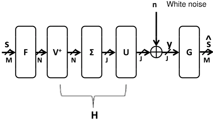
The GTD can also be viewed as triangularization of the input matrix Hby two semi-unitary matrices (PandQ) on both sides. There are many standard decompositions that can be regarded as special instances of the GTD. These are listed below. The first five can be found in standard texts [25, 31], while the sixth was proposed by Jiang et. al. in the context of MIMO transceiver optimization.

1. Thesingular value decomposition(SVD),H=UΣV† whereΣis a diagonal matrix containing the singular values on the diagonal.

2. TheSchur decomposition,H=Q∆Q†where∆is an upper triangular matrix with eigenvalues of a square matrixHon the diagonal.

(42)

4. Thecomplete orthogonal decomposition,H=Q2R2Q†1, whereH† =Q1R1is the QR factoriza-tion ofH†andR†₁=Q2R2is the QR factorization ofR†1.

5. Thebidiagonal decomposition,H=QBP†, whereBis a bidiagonal and upper triangular matrix (page 251 of [25]).

6. Thegeometric mean decomposition(GMD) [36],H=QRP†whereRis an upper triangular ma-trix with the diagonal elements equal to the geometric means of the positive singular values.

The computation of performing GTD has the same asymptotic complexity as the singular value decomposition [38]. Jianget. al. provided a numerically stable algorithm to compute any GTD with prescribed diagonal elements as long as the multiplicative majorization relation is satisfied. The algorithm starts by performing the singular value decomposition to obtain the diagonal matrix with singular values on the diagonals. Then, successive Givens rotations are performed to produce the middle upper triangular matrix with prescribed diagonal elements. Note that the singular values are invariant under Givens rotations. The details of this algorithm and a computer code implementation can be found in [38].

2.3.1

Block-Diagonal Geometric Mean Decomposition

The block diagonal geometric mean decomposition (BD-GMD) is a special case of the GMD. In BD-GMD, one of the unitary matrices in (2.4) is restricted to be block diagonal. The price paid is that the diagonal elements of the middle triangular matrix can no longer be made equal. Instead, they are block-wise equal. To be more specific, consider the matrix decomposition of the following form. SupposeH∈Cm×n_{is with full column rank}_n_{and we are seeking the decomposition}

H†=PLQ†,

whereQis am×nmatrix with orthonormal columns,Lis an×nlower triangular matrix, andP

is an×nblock diagonal matrix of the form diag(P1,P2,· · · ,PK)where each blockPiis a unitary

ni×nimatrix. The task is to find a matrix decomposition such that the diagonal elements ofLare

equal in blocks ofn1,· · · , nK elements respectively. This decomposition was proposed by Linet.

(43)

The algorithm proposed by [47] is as follows. First, rewrite the decomposition as 



H†₁

H†r

 =

 

P1 0

0 Pr

 

 

L1 0

A Lr

   

Q†₁

Q†r



 (2.5)

whereH†₁andQ†₁aren1×msubmatrices, andL1andP1aren1×n1square matrices.H†rdenotes

the remaining lower part of the matrixH†. Expanding the above equation gives the following two equations

H†₁=P1L1Q†1 (2.6)

and

H†_r=PrAQ†1+PrLrQ†r. (2.7)

From Equation (2.5), it can be seen that by performing the GMD, the diagonal elements ofL1 can be made equal. SinceQhas orthonormal columns, the submatricesQ1andQrare orthonormal

to each other. Thus, from Equation (2.7), multiplication by the projection matrixI−Q1Q

†

1gives

H†_r(I−Q1Q1†) =PrLrQ†r.

Here, the right side of the above equation has the same form as in (2.5), so the algorithm proceeds recursively. To solve forA, equation (2.7) is multiplied byP†randQ1 on the left and right hand side, respectively, giving

A=P†_rH†_rQ1.

This decomposition then has equal diagonal elements in each block of L. After performing the BD-GMD, the matrixH†can be decomposed as follows:

H†=

       

H†₁

H†₂

.. .

H†_K

        =         

P1 0 · · · 0

0 P2 . .. ... ..

. . .. ... 0 0 · · · 0 PK

        

| {z }

P         

L1 0 · · · 0

× L2 . .. ... ..

. . .. ... 0 × · · · × LK

        

| {z }

L        

Q†₁

Q†₂

.. .

Q†_K

        | {z }

Q†

(44)

(45)

Chapter 3

Transceiver Designs for MIMO

Frequency Flat Channels

In this chapter we consider the optimization of transceivers for frequency flat MIMO channels. The first part of this chapter studies the optimization of MIMO transceivers with linear precoders, decision feedback equalizers, and bit allocation schemes. Considered first is the minimization of the average transmitted power, for a given total bit rate and a specified set of error probabilities for the symbol streams. While this joint optimization has not been addressed in the past, a variety of related transceiver designs have been studied previously. When the transmitter has perfect channel information, four major optimization problems have been considered. First, for fixed precoder and DFE matrices, the optimal bit loading problem has been studied in [9]. Second, for the case where the bit allocation is fixed to be uniform, joint optimization of the precoder and DFE matrices is a well studied problem [36, 37, 41, 90, 137, 142]. Third, for the case of linear transceivers, the joint optimization of the precoder, the (linear) equalizer, and bit allocation has been studied in [48] (under ZF constraint), and in [74] (without ZF constraint). Fourth, if the precoding matrix is restricted to be a diagonal matrix where only power loading applies, the optimization of rate and power allocation for the systems with DFE receiver has been discussed in [14]. If no perfect channel state information is present (only channel statistics known at the transmitter), the optimization of power and rate allocation for the system with DFE receiver was addressed in [83].

(46)

decom-position (GTD) introduced in [38] offers an optimal solution. The GTD in fact gives rise to a family of solutions, with the bit allocation details changing from solution to solution. We will see in par-ticular that the optimal linear transceiver with optimal bit allocation, which has alinearequalizer rather than a DFE, is a member of this family of solutions. This shows formally that, under optimal bit allocation, optimum linear transceivers achieve the same transmitted power as optimum DFE transceivers with bit allocation. These discussions assume that the bit allocation formula is real-izable (i.e, the bits are nonnegative integers). The DFE transceiver based on the geometric mean decomposition (GMD) [36] is another member of the above family of optimal solutions, and is such that the optimal bit allocation formula yieldsidentical bits for all symbol substreams, when the specified error probabilities are identical for the substreams. DFE with GMD therefore achieves minimum power even without the need for bit allocation. In a way this complements one of the results in [36], namely, when all symbol streams are constrained to have identical bits, the average bit error rate (BER) for fixed power is minimized by the GMD. Other special cases arising from the GTD family of optimal DFE systems include the VBLAST system [135], and a new solution called the bidiagonal (BID) transceiver. Two other optimization problems are then considered: (a) mini-mization of power for specified set of bit rates and error probabilities (the QoS problem), and (b) maximization of bit rate for a fixed set of error probabilities and power. It is shown in both cases that the GTD yields an optimal family of solutions.

The second part of this chapter considers the joint transceiver optimization problem for fre-quency flat MIMO channels under other constraints. The linear transceiver as well as the DFE transceiver are considered. Instead of only the total power constraint, in this section we also con-sider the more realistic per-antenna power constraints on the transmitter [45, 139]. This is because in practice each antenna is limited individually by its equipped power amplifier. In [45], the MMSE problem under individual power constraints is solved sub-optimally using a numerical approach. In [139], the multiuser down-link transceiver design problem is considered. The total power con-straint might still be needed since the antennas might rely on a common power supply. Under these constraints, we consider the linear transceiver case and also the simple nonlinear case, i.e., linear precoding with DFE at the equalizer.

(47)

In [73], the authors considered only Schur-concave objective functions subject to the individual power constraints. However, the problem of optimizing the transceiver for other important ob-jective functions (e.g., Schur-convex functions, including average BER) was not addressed. Direct use of the results of [73] to address this case is nontrivial. In [76] the author considered shaping constraints on the transmitted signal covariance matrix. However, as acknowledged by the author in [76], the paper introduced a stronger artificial constraint that leads to a sub-optimal solution.

Our work is to tackle these unsolved problems in the literature. For the linear transceiver case, we first consider the minimum AM-MSE (Arithmetic Mean of Mean Square Errors) design. We show that it can be reformulated as a semi-definite program (SDP), which can be solved nu-merically by convex optimization tools. Then, among the family of minimum AM-MSE linear transceivers, we develop a method to find the one that minimizes the average bit error rate as well as many other objective functions. This second step is achieved by appealing to majorization the-ory. Similarly, for the transceivers with linear precoding and DFE, we first consider the minimum GM-MSE (Geometric Mean of Mean Square Errors) design. We show that it can also be reformu-lated as an SDP, and solved efficiently. Then, among the family of minimum GM-MSE designs, we develop a method to find the one that minimizes the average bit error rate as well as many other objective functions.

Based on majorization theory [65], we will argue that the minimal average BER transceiver design method developed in this section can also be applied to a wider class of objective functions. Also, we will show that under the framework developed here, any additional linear constraints on the covariance matrix of the transmitted signals can be further added, and the problem is solved both in theory and practice with no difficulty. Examples of such constraints may be spatial power masks. This was formulated but not elaborated in [76]. In addition, it is shown in Section 3.3.5 that our framework includes the case studied in [76].

The content of this chapter is mainly drawn from [123, 128], and portions of it have been pre-sented in [119, 120, 125].

3.1

Outline

(48)

covariance matrix, including total power constraint and individual antenna power constraints. Fi-nally, the conclusions are made in Sec. 3.4.

3.2

MIMO Transceivers with Decision Feedback and Bit Loading

In this section, we consider MIMO transceivers with a linear precoder and a decision feedback equalizer (DFE), with bit allocation allowed at the transmitter end. Zero-forcing and QAM sig-naling are considered throughout, and the perfect channel information is assumed to be known to the transmitter and the receiver. This section is structured as follows. In Sec. 3.2.1, we formulate the power minimization problem. In Sec. 3.2.2, we show that under optimal bit allocation, opti-mum linear