Circuit breaker simulated operation & behaviour under faulted power system conditions

(1)

University of Southern Queensland

Faculty of Health, Engineering & Sciences

Circuit Breaker Simulated Operation & Behaviour Under

Faulted Power System Conditions

A dissertation submitted by

B. Wentworth

in fulfilment of the requirements of

ENG4112 Research Project

towards the degree of

Bachelor of Power Engineering

(2)

Abstract

The rapid increase in electrical demand and supply reliability for both domestic and

industrial use throughout the modern world provides a set of unique challenges for supply

authorities. It is not only paramount that the ever increasing supply and reliability

demands are met but also environmental and cost concerns are addressed.

It has been proven that single pole tripping and reclosure schemes implemented on EHV

(Extra High Voltage) transmission lines greatly aid in both supply availability and

reli-ability. However, it is obvious that such schemes will greatly increase the complexity to

both the primary and secondary systems. Subsequently, it is clear that the behaviour of

the primary network under single pole operation must be extensively modelled to enable

adequate protection and control by secondary protection systems.

Throughout the following study a technique for determining the maximum fault duration

on a transmission network that incorporates single pole tripping has been developed.

Fur-ther to this, investigations into accurate modelling of the physical network particularly

pertaining to the fault arc that will be seen inside an EHV circuit breaker when

open-ing under faulted network conditions has been undertaken. These techniques have been

utilised to produce a specific maximum fault duration of 57ms for an example case study;

subsequent circuit breaker failure times were then developed for a number of protection

(3)

University of Southern Queensland Faculty of Health, Engineering & Sciences

ENG4111/2 Research Project

Limitations of Use

The Council of the University of Southern Queensland, its Faculty of Health, Engineering

& Sciences, and the staff of the University of Southern Queensland, do not accept any

responsibility for the truth, accuracy or completeness of material contained within or

associated with this dissertation.

Persons using all or any part of this material do so at their own risk, and not at the risk of

the Council of the University of Southern Queensland, its Faculty of Health, Engineering

& Sciences or the staff of the University of Southern Queensland.

This dissertation reports an educational exercise and has no purpose or validity beyond

this exercise. The sole purpose of the course pair entitled “Research Project” is to

con-tribute to the overall education within the student’s chosen degree program. This

doc-ument, the associated hardware, software, drawings, and other material set out in the

associated appendices should not be used for any other purpose: if they are so used, it is

(4)

Certification of Dissertation

I certify that the ideas, designs and experimental work, results, analyses and conclusions

set out in this dissertation are entirely my own effort, except where otherwise indicated

and acknowledged.

I further certify that the work is original and has not been previously submitted for

assessment in any other course or institution, except where specifically stated.

B. Wentworth

(5)

Acknowledgments

First and foremost I would like to thank my supervisor Dr Tony Ahfock for his unwavering

support and assistance throughout the entire dissertation process; without his invaluable

assistance the completion of this dissertation would not have been possible.

Secondly, I would like to thank my family; Heather, Greg, Megan and Laura for the

support and encouragement shown when the demands of this dissertation appeared too

great.

(6)

List of Figures

2.1 Simplified Network Impedance Diagram. . . 6

2.2 Simplified Network Impedance Diagram - Fault Location. . . 8

2.3 (a) Negative Sequence Diagram. (b) Zero Sequence Diagram . . . 8

2.4 (a) Combined Sequence Diagram.(b) Simplified Combined Sequence Diagram 9 2.5 Fault Oscillogram (Courtesy Sing Wai Mak, Ausnet Services). . . 11

4.1 PI Line Model Diagram (Mathworks(b) 2016). . . 23

4.3 Simplified Network Diagram. . . 26

4.4 Single Line Diagram - Fault Locations. . . 32

5.1 Cassie Model - Current Chopping . . . 40

5.2 Mayr Model - Current Chopping . . . 40

5.3 Mayr Model - 0 Ω Impedance . . . 42

5.4 Mayr Model - 1000 Ω Impedance . . . 43

5.5 Mayr Model - 0MW Load . . . 45

(12)

LIST OF FIGURES xii

5.7 Positive DC Offset . . . 47

(13)

List of Tables

2.1 Summary Systemδ With Respect to System Impedance Change. . . 9

2.2 Summary of System Stability With Respect toδ. . . 10

3.1 Short Circuit Ground Fault Levels. . . 15

4.1 Example Line Loading Records. . . 25

4.2 500kV Circuit Breaker Recorded Operation Times. . . 27

4.3 500kV Protection Device Recorded Operation Times. . . 27

5.1 Results Summary - Start of Line - Table. . . 35

5.2 Results Summary - Middle of Line - Table. . . 36

5.3 Results Summary - End of Line - Table . . . 36

5.4 Mayr vs. Cassie Effect On Fault Duration . . . 37

5.5 Arc Model Effect On Fault Current Magnitude . . . 38

5.6 Mayr vs. Cassie Effect On Fault Current Magnitude . . . 38

5.7 Arc Model Effect On Post Fault Current Magnitude . . . 39

(14)

LIST OF TABLES xiv

5.9 Impedance Effect On Time . . . 41

5.10 System Load Effect On Time . . . 44

5.11 System Load Effect On Fault Current . . . 44

5.12 Post Fault Current . . . 45

B.1 Results - DT - Start of Line - Table. . . 60

B.2 Results - Mayr - Start of Line - Table. . . 61

B.3 Results - Cassie - Start of Line - Table. . . 62

C.1 Results - DT - Middle of Line - Table. . . 64

C.2 Results - Mayr - Middle of Line - Table. . . 65

C.3 Results - Cassie - Middle of Line - Table. . . 66

D.1 Results - DT - End of Line - Table. . . 68

D.2 Results - Mayr - End of Line - Table. . . 69

(15)

Chapter 1

Introduction

The following chapter is comprised of three sections; firstly, the justification and reasoning

behind the need for this dissertation are discussed, secondly, the overall objectives are

outlined and described, and finally, the prerequisites will be defined.

1.1

Project Justification

As global population and standard of living continue to rapidly increase it is obvious and

indisputable that the demand for electricity will also continue to increase. In addition to

this consumption accretion both household and industrial consumers are also expecting

an ever increasing level of supply reliability.

In many cases these large increases in demand will put additional strain on aging power

system equipment that is already heavily loaded. This will evidently reduce the level of

reliability achieved.

The foremost solution would be to install additional transmission and distribution

equip-ment that achieve very high levels of system redundancy. However this solution is not

practicable for two main reasons: firstly, society’s ever increasing environmentalist

influ-ence demands the reduction in destruction of flora; secondly, the increase in construction

costs predominantly driven by inflation and the rise of wages have imposed heavy

(16)

1.2 Objectives 2

The above restrictions have subsequently forced many distribution and transmission

com-panies to seek and develop technologies that can supply large amounts of reliable power

using fewer transmission lines, which will thereupon reduce both environmental damage

and costs.

In an attempt to meet the requirements and restrictions outlined above, transmission

companies must essentially have fewer transmission lines that are capable of supplying

very large amounts of power. This is achieved by installing EHV (Extra-High Voltage)

lines which become backbones to the electricity network.

As the amount of power transported by these network backbones is so great it is

abun-dantly clear that additional reliability measures must be taken to prevent mass outages in

the case of an unexpected system event. This additional reliability on the EHV network

is often achieved by the application of single pole tripping.

Although single pole tripping increases reliability it also important to note that it greatly

increases the complexity of system events and related protection and control devices.

It is clear from the above paragraphs that there is a need to determine, understand and

model the behaviour of three phase networks that operate with a single pole tripping

scheme.

1.2

Objectives

The overall aim of this dissertation is to give a detailed study of single pole circuit breaker

operation and arcing characteristics under faulted power system conditions. Arcing

char-acteristic models will be combined with power system network models for the purpose of

determining the realistic clearance time for a high voltage circuit breaker, from fault

ini-tiation to fault clearance under various network configurations/conditions; subsequently

applying these findings to a three phase network where minimal clearance and circuit

breaker failure times are required to ensure network stability. The six following points

outline the main project objectives.

A) Examine existing information on EHV (Extra High Voltage) CB (Circuit Breaker)

(17)

1.3 Resource Requirements 3

B) Determine the characteristics of three (3) phase (single pole operated) EHV CBs.

C) Utilise EHV CB models to simulate a power network that can achieve the single pole

tripping characteristics defined in objective B

D) Determine a realistic fault characteristic for a single phase fault in a three phase power

system.

E) Utilise a realistic arc model under various system faulted conditions.

F) Analyse fault clearance times to determine a realistic circuit breaker failure time.

1.3

Resource Requirements

The network simulation including all EHV CB arc modelling and fault modelling is to

be implemented using Mathworks Simulink Simscape Power Systems. Existing Mayr and

Cassie arc models were available from Mathworks(a) (2016).

1.4

Chapter Summary

This introductory chapter has provided the justification and project objectives. Firstly

the increase in consumer demand and reliability expectation was discussed; this

subse-quently led into the justifications behind utilising single pole tripping schemes rather than

installing new transmission and distribution equipment. Secondly, the overall aim and

(18)

Chapter 2

Background

The following chapter is comprised of two main sections; technical background and fault

data. The first section describes the operational behaviour of a single pole scheme and

gives a detailed example of the improvements seen when using a single pole network;

the second section contains a record of a single phase to ground fault that is to be used

extensively to determine EHV CB characteristics and parameters.

2.1

Technical Background

Throughout the following section a discussion focusing on the behaviour and

charac-teristics of a single pole circuit breaker utilised within a three phase network will be

undertaken; this dialogue will contribute towards meeting the requirements of objective

B. Furthermore, an in-depth investigation and subsequent case study into the effect single

pole circuit breakers have on network stability will be carried out.

2.1.1 Circuit Breaker Operation

A protection and control scheme that incorporates single pole tripping will initially detect

a fault within the protected object or zone as per any standard 3 pole scheme. However

after this initial fault detection the protection device will then determine what type of

fault is occurring and the number of phases involved. If it is determined that a phase to

(19)

2.1 Technical Background 5

leaving the remaining two phases closed and supplying load. When a two phase or three

phase fault is detected then a protection trip will be issued to all poles.

It is important to note that whenever a single pole trip is issued a re-closure initiate for

that pole is also issued as the network is not designed to run on two phases alone; the

reasoning behind this will be discussed and justified in detail later in this section.

As a generalised statement single pole schemes will use the below pro forma;

Single phase fault: the faulted phase is tripped and reclosed after a pre-defined dead time.

If the fault has been cleared then the system returns to stable conditions. If the fault has

not cleared after this dead time then the remaining two phases will be tripped. This will

cause both a single pole and three pole reclose lockout. It is also important to implement

a single pole circuit breaker fail scheme. In this scenario a single pole trip has been issued

and the pole has not opened; after a predetermined breaker failure time a three pole trip

must be issued to the original circuit breaker and the backup breaker/s upstream. The

variation from a normal breaker failure scheme is that even under correct operation of a

single pole trip the remaining two phases will continue to carry load current. Because of

this load current each pole must have an individual current check to correctly assess the

breaker failure conditions.

Two phase and three phase faults will trip all three poles and will be reclosed after a

predetermined dead time. If the fault has been cleared then the system returns to stable

conditions. If the fault has not cleared after this dead time then all three poles will be

tripped and no further reclosure will take place. As per any three pole scheme if a trip

is issued and the fault has not been cleared within a pre-determined time circuit breaker

fail initiate will be issued.

Evolving faults must also be given consideration when implementing single pole tripping.

Evolving faults start as a single phase to ground fault and then involve other phases

before that fault is cleared. As single pole protection schemes have protection on a per

pole basis they will inherently have some capability to deal with faults evolving; however

additional logic is required to ensure that a three pole trip is issued when the second

individual pole fault detector is active. This is a built in function in almost all modern

(20)

2.1.2 Network Stability

Ngamsanroaj & Watson (2014) state that over 90% of transmission line faults are phase

to ground and transient. Following this reasoning it is of no surprise that modern power

networks implement single pole tripping schemes. These schemes are utilised to increase

the reliability and availability of mesh transmission systems. It is blatantly obvious that

the degree of which single pole tripping can improve the reliability of a mesh network is

dependent on how that particular mesh network is configured.

In any case single pole tripping will increase the reliability of any network as when a

single pole is tripped the increase of network impedance is much less than that of a three

pole trip. AEMO (2013) show that the Victorian transmission network has a 500kV

backbone that not only runs the entire length of the state but also interconnects with

South Australia and New South Wales. It is obvious that such a intergral component

of the transmission network will require the highest level of reliability available; this

backbone has two parallel 500kV lines that implement single pole tripping at all terminal

locations. Utilising the methodology outlined in GE Group (2002) in combination with

the network parameters obtained from the Victorian transmission authority the following

example will demonstrate the necessity for single pole tripping within the EHV Victorian

[image:20.595.135.455.504.582.2]

mesh network.

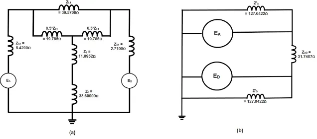
Figure 2.1: Simplified Network Impedance Diagram.

Figure 2.1 can be considered a simplified version of a section within the Victorian

back-bone. The maximum power that can be delivered can be easily obtained by:

PM AX =

E2

X (2.1)

WherePM AX is the maximum power the network can deliver, E2 is the constant system

(21)

Equation 2.1 is the theoretical steady state stability limit, and will occur when the voltage

at source EA leads the voltage at source ED by 90 degrees. It is widely known that

networks do not operate at the steady state stability limit. Equation 2.1 can be expanded

into 2.2 to represent a more realistic power transfer across the system.

P = EAED

XAD

Sin(δ) (2.2)

Where EA is the phase to phase transmission voltage at A, ED is the phase to phase

transmission voltage at D,XAD is the system reactance between A and D, finallyδ is the

angle EA leadsED.

Due to the heavy level of voltage regulation throughout the network we can assume that

the voltages at source A and D are held constant. This gives a relationship where the angle

between the two voltages is directly related to the power flow. The higher the system

reactance, the higher the angle between the two voltage sources. Hence as described above

the lower the change of system reactance the greater the stability of the system.

For the purposes of this example the following assumptions have been made: the line

characteristics of line B and line C are identical (ZB =ZC =ZL), impedanceZAis equal

to 20km of the total line impedance for one line and impedance ZD is equal to 10km of

the total line impedance for one line.

The following data about a specific section of the Victorian 500kV network has been

obtained from the transmission authority: positive sequence impedance for entire line

as 39.57Ω, zero sequence impedance for entire line as 112.02Ω and the line length as

146km. Hence ZL1 = 39.57Ω and ZL0 = 112.02Ω. Subsequently the following can easily

be obtained:

ZA1= 20∗ ZL1

l (2.3)

ZA0= 20∗ ZL0

l (2.4)

ZB1 = 10∗ ZL1

l (2.5)

ZB0 = 10∗ ZL0

(22)

Where lis the 146km length of the line.

Using equations 2.3, 2.4, 2.5 and 2.6 we can determineZA1as 5.4200Ω/km,ZA0as 15.3460Ω/km,

ZB1 as 2.7100Ω/kmandZB0 as 7.6730Ω/km.

ZAD−N ormal =ZA1+

ZL1

2 +ZD1 (2.7)

Equation 2.7 shows the effective impedance between the two sources under normal

oper-ational conditions and can easily be determined as 27.9150Ω.

ZAD−Single−Line=ZA1+ZL1+ZD1 (2.8)

Equation 2.8 describes the effective impedance between the two sources with one line in

service. This situation would occur when a three pole trip has occured on one of the lines

with the other remaining in service. Equation 2.8 can be determined thatZAD−Single−Line

[image:22.595.141.458.432.519.2]

is equal to 47.7Ω.

Figure 2.2: Simplified Network Impedance Diagram - Fault Location.

Now consider Figure 2.2 which indicates a single phase to ground fault in the centre of

one of the transmission lines. When analysing a phase to ground fault positive, negative

and zero sequence networks must be be analysed.

Figure 2.3: (a) Negative Sequence Diagram. (b) Zero Sequence Diagram

(23)

and series reduction the negative sequence impedance can be reduced to a single value of

11.8592Ω. While Figure 2.3 (b) shows the negative sequence impedances, using delta-star

transformation and series reduction the negative sequence impedance can be reduced to

[image:23.595.138.456.179.319.2]

a single value of 33.6000Ω

Figure 2.4: (a) Combined Sequence Diagram.(b) Simplified Combined Sequence Diagram

Figure 2.4 (a) shows the combined sequence diagram. This diagram incorporates all

three sequence networks; however it must be simplified to be of any real use. Performing

successive star delta transformation in combination with series reduction on Figure 2.4 (a)

we can obtain Figure 2.4 (b). As Figure 2.4 (b) shows the combined sequence impedance

can be simplified down three values, however as we are attempting to determine the

impedance between the sources it is clear that we only require ZAD which has been

simplified to 31.7407Ω. In this instance we will assume that the resistive component is

negligible, hence; ZAD=XAD

Using equation 2.2 the table 2.1 can be created:

Table 2.1: Summary Systemδ With Respect to System Impedance Change.

Case ZAD δ

2 lines in service (normal conditions) 25.92 Ω 24.50◦

2 lines in service (A-G fault - 1 pole trip) 31.74 Ω 30.52◦

2 lines in service (A-G fault - 3 pole trip) 47.70 Ω 49.75◦

Using the simplified equal area stability equations determined in GE Group (2002) we

get the following stability equation:

E2 Xb

(24)

2.2 Fault Data 10

Where E is the constant system voltage, Xb is the system impedance after breaker

op-eration, δ1 is the angle of the system before the breaker operation,δ2 is the angle of the

system after the breaker operation andPT is the total power flowing through the system

at the time of the breaker operation.

Table 2.2 can be developed by applying equation 2.9 to each of the circuit breaker

oper-ation scenarios. Equoper-ation 2.2 has been used to determine a realistic power flow of 4000

MW at the time of fault.

Table 2.2: Summary of System Stability With Respect toδ.

Case Equation Results System

2 lines in service (A-G fault - 1 pole trip) 13952 MW> 8725 MW Stable

2 lines in service (A-G fault - 3 pole trip) 8156 MW>7383 MW Stable

Whilst it can be seen that under the given conditions the system will remain stable for

both a single pole and three pole trip, it is clear that the system maintains a much higher

level of stability for a single pole trip. It is also important to note that if the system were

to be subjected to above normal loading conditions then a three pole trip on one line may

result in the system becoming unstable.

2.2

Fault Data

Fault records obtained from the Victorian 500kV transmission network will be used to

obtain numerous parameters for the simulated network. By obtaining parameters from

actual fault data a more realistic model can be produced using less assumptions, this will

aid in meeting objectives B and D. The fault oscillogram in figure 2.5 has been extracted

from a recording device that was monitoring a 550kV, 63kA, 50Hz circuit breaker. This

type of breaker is used extensively throughout this and many other EHV networks.

The values obtained from the fault oscillogram will be measured and used for validation

and verification of the calculated fault model used within this study. Figure 2.5 is a

captured fault record of a single phase to ground fault on the Victorian EHV network

and is suitable for the purposes of this study as all simulated faults are of a single phase

(25)

[image:25.595.128.465.90.468.2]

2.3 Chapter Summary 11

Figure 2.5: Fault Oscillogram (Courtesy Sing Wai Mak, Ausnet Services).

It can readily be seen that the fault oscillogram in Figure 2.5 comprises of four

compo-nents; F1-A shows the recorded A phase faulted line current, F5-VA indicates the A phase

faulted line voltage, 87L DIFF OP A illustrates when the differential protection element

operated and BREAKER 1 CLOSED describes the A phase CB closed status.

The current zero for this fault occurs 53.13 ms after fault inception and 29.38 ms after

protection relay operation.

2.3

Chapter Summary

The background chapter is comprised of two major sections; the first section contains a

technical background and provides a detailed example of the benefits seen when utilising

(26)

2.3 Chapter Summary 12

record from an in service protection device that has been subject to a single phase to

ground fault; this record will be utilised within later chapters to establish realistic circuit

(27)

Chapter 3

Literature Review

The following section is an overview of the literature used to determine the

characteris-tics and behaviour of SF6 CB’s within an EHV network. This section will address the

behaviour of extra high voltage circuit breakers particularly pertaining to arcing during

faulted network conditions. It is the aim of the report to use these previous studies as a

benchmark for determining methods to obtain realistic fault simulation and subsequently

fault clearance times.

3.1

Circuit Breaker Characteristics

The following section discusses the characteristics of an EHV CB; subsequently it is an

important component in meeting the requirements of objective B. Firstly it is important

to consider how and why an EHV CB will operate. When a fault occurs on an EHV

network a protective device will detect the faulted condition and then initiate a trip to

the EHV CB. This trip initiate will effectively begin the process of parting of the EHV CB

contacts. Whilst the time taken for the CB contacts to physically part is extremely quick

(a matter of milliseconds) it is still long enough for an arc to form. There are numerous

types of insulation materials used by manufacturers of EHV CB’s; however the current

leader in insulation material is SF6. Subsequently this study will focus on EHV CB’s

(28)

3.2 Transmission Line Characteristics 14

Oh, Y. and Song, K. (2015) describe that when analysing current interruption inSF6CB’s

it is important to consider the arc plasma generated between the separating contacts. This

plasma will be at a temperature of many thousands of degrees, encompass high electric

field conduction as well as super and sub sonic gas flows . The aforementioned factors

all hinder in the extinguishing of the arc. With this in mind the overall concept of

arc extinction is still relatively simple; the arc resistance increases as the contacts part,

when this arc resistance is large enough the arc current is interupted, this is particularly

prevalent at the zero crossing. Conversely if the resistance is not large enough directly

after a zero crossing occurs the arc will be re-ignited and the fault will continue.

3.2

Transmission Line Characteristics

To determine which line parameters are necessary to accurately model a single phase to

ground fault we must first look at how the line will behave under faulted conditions; these

line characteristics will aid in meeting the requirements of objective A and B. Jannati,

Vahidi, Hosseinian & Ahadi (2011) describe that when a system is healthy and a phase

to ground fault occurs two distinct arcs will be seen, a primary arc and a secondary arc.

The Primary arc is essentially caused by a short circuit that has been formed when

one phase of a healthy system is faulted to earth. Arc quenching will be discussed in

much greater detail throughout this report; however for the purpose of determining line

parameters the primary arc can be considered quenched when the contacts of the high

voltage circuit breaker on the faulted phase are fully opened. After the aforementioned

primary fault has been cleared by the operation of the high voltage circuit breaker it will be

assumed that the two non-faulted phases will remain closed and supplying load. Jannati

et al. (2011) state that due to the two healthy phases remaining closed a capacitive

coupling effect will be seen and the faulted phase may then produce a secondary arc.

It is well known that to effectively model any electrical circuit the impedance must be

known, transmission lines are no exception. However, as justified in the above paragraphs,

to accurately model a line with single pole tripping it is not only essential to have accurate

line impedance values but effectively represent the capacitive coupling effect.

Pinto, Costa, Kurokawa, Monteiro, de Franco & Pissolato (2014) describe in great detail

(29)

3.3 Network Fault Levels 15

and also the spacing between conductors; in particular how multiconductor transmission

systems can be represented by an impedance matrix [Z] and admittance matrix [Y].

However they continue to describe that whilst maintaining sufficient accuracy these two

multiconductor matrix’s can be simplified into four sequence component value; positive

sequence capacitive reactance (XC1), zero sequence capacitive reactance (XC0), positive

sequence impedance (Z1) and zero sequence impedance (Z0).

3.3

Network Fault Levels

To accurately and effectively model any fault and meet the requirements of objective B

and C it is important to determine the perspective maximum short circuit level at that

particular point in the network. These short circuit levels are expected to be much larger

than the network has been designed to handle continuously. Perspective maximum short

circuit levels are determined by the voltage and the impedance of the system and are

essentially considered as the maximum amount of current that can be delivered at the

specified point in the network.

The 500kV network that has been used for validation throughout various stages of this

report is a critical component to the Victorian transmission network; AEMO (Australian

Energy Market Operator) have publically released the short circuit fault values for all

major terminal stations throughout the entire Victorian backbone. The relevant short

circuit values from AEMO (2012) have been summarised in table 3.1.

Table 3.1: Short Circuit Ground Fault Levels.

Station Pre-Fault Voltage Ig Deliverable Power

MLTS 520.6 kV 15.5 kA 8069.3 MVA

MOPS 527.5 kV 9.5 kA 5011.3 MVA

TRTS 526.0 kV 7.5 kA 3945.0 MVA

APD 520.5 kV 8.8 kA 4580.4 MVA

HYTS-B1 523.6 kV 8.5 kA 4450.6 MVA

(30)

3.4 Network Loading Effects 16

3.4

Network Loading Effects

Goday, E. and Celaya, A (2012) describe how a three phase transmission line will be

subjected to both electromagnetic and electrostatic coupling during its normal operational

conditions. It is subsequently obvious that these coupling effects will remain whenever all,

or part of the transmission line is energised. Hence, it is clear that to achieve objective

C these coupling effects must be considered in detail.

As described previously, when a single phase to ground fault occurs a primary arc is

formed. The protection device will then initiate a single pole trip on the faulted phase.

The un-faulted phases will remain closed and continue to supply load. It is because of

this load voltage and current within the two un-faulted phases that electromagnetic and

electrostatic coupling induce a voltage and subsequent current on the now open phase.

Electrostatic coupling is commonly called capacitive coupling and can essentially be

de-scribed as a function of the line voltage and physical line characteristics. The line

capac-itance is a combination of the distance between each of the phases and also the distance

of the phase conductors to the ground.

Goday, E. and Celaya, A (2012) have developed equation 3.1 to determine the electrostatic

secondary arc current and equation 3.2 to represent the recovery voltage.

IARC−C =VLN∗jωCm (3.1)

VREC =VLN

Cm

(2Cm+Cg)

(3.2)

WhereVLN is the line to neutral voltage,Cm is the equivalent capacitance between phases

and Cg is the capacitance to ground. From the relationship defined in 3.2 it is easy to see

that higher line voltages will produce higher levels of electrostatic coupling.

NTT Technical (2007) describe that electromagnetic induction is caused by alternating

current inducing a magnetic field around the conductor it is flowing through. When

another conductor is within this induced magnetic field it will then be subjected to the

(31)

3.5 Definite Maximum Fault Time 17

describing how electromagnetic induction is a function of the load current and the total

distance that the conductors are paralleled. In the situation of a single phase trip the

conductors will obviously be parallel for the entire lenth of the line.

From the above paragraphs it is clear that the line voltage and current in the un-faulted

phases will create an electrostatic and electromagnetic coupling effect in the recently

opened faulted phase. It is clear that the larger the voltage and current of the un-faulted

phases the larger the coupling effect. Hence loading on the transmission line will play a

large role in the TRV (transient recovery voltage) seen.

3.5

Definite Maximum Fault Time

Clearly it would be ideal if the detection of a fault by a protective device and the operation

of a high voltage circuit breaker happened instantaneously; however, in reality neither of

these hold true.

When considering the realistic operation time to clear a faulted circuit, it is first important

to consider what actually causes the interruption of current. The actual interruption

device is a EHV CB. However for this interruption to occur a protective device must first

initiate the operation. When a fault is present and detected by a protective device it will

issue a trip to the EHV CB. Although both protection operation and EHV CB operation

speeds are increasing as technology advances both of these aspects still take some physical

time to complete and cannot be considered instantaneous.

It can then be said that with a very simplistic view when a EHV CB’s contacts are fully

open that any fault that was present will be cleared. For the purpose of this section of

the study it will be assumed that the EHV CB’s are of adequate rating to interrupt any

fault and that all faults will be cleared when the circuit breaker contacts are fully open.

With this assumption in mind the time of the fault is then limited to the initial detection

time of the protection device plus the time it takes for the contacts of the EHV CB to

fully open. This time will be called the definite maximum fault time. In reality, the fault

may be broken before this time or not at all; earlier arc interruption will be discussed in

(32)

3.6 Arc Models 18

3.6

Arc Models

Literature relating to two prominent arc models will be discussed throughout the following

section. In the first subsection Mayrs arc model will be analysed; the second will discuss

Cassies arc model. To meet objective D it is the intent of this study to perform analysis

using both arc models with the desire to then compare the results.

3.6.1 Mayr Arc Model

Schavemaker & van der Slui (2000) defines the Mayr arc as equation 3.3, where G is the

arc conductance,um is the arc voltage,im is the arc current,τm is the arc time constant

and P0 is the cooling power.

1 G dG dt = dlnG dt = 1 τm

(um∗im

P0 −1) (3.3)

The Mayr model assumes that the thermal conduction at small currents is the cause of

power loss. It can then be said that the arc conductance is highly temperature dependant.

Further to this it can be determined that the arc conductance depends very little on the

cross sectional area; subsequently the cross sectional area of the arc will be assumed as a

constant. In addition to the above assumptions Mayr states that the relationship between

the voltage and current is constant; hence P0 is equal to PLOSS and is to be considered

constant. When there is no power input to the arc (zero crossing) τm is time constant of

the change in temperature.

P =ui (3.4)

Using the fundamental relationship in equation 3.4 we can simplify equation 3.3 to obtain

3.5: 1 G dG dt = dlnG dt = 1 τm ( P PLOSS

−1) (3.5)

(33)

3.7 Arc Conductance 19

throughout the iterative process, howeverPLOSS is a constant that must be known prior.

3.6.2 Cassie Arc Model

Bizjak, Zunko & Povh (1995) defines the Cassie arc as equation 3.6, where Uc is the arc

voltage andτcis the arc time constant.

1

G dG

dt =

1

τc

(u

2

U2

c

−1) (3.6)

The Cassie model assumes that convection is the only cause of power loss in the arc.

Subsequently it can assumed that the temperature in the arc is constant. Further to this

it can be determined that the cross sectional area of the arc is proportional to the current.

By inspection of equation 3.6 it is clear thatucan be determined and will vary throughout

the iterative process, howeverUcis constant and must be known prior.

3.7

Arc Conductance

It is quite obvious that the breaking ability of a circuit breaker will depend on a multitude

of factors. Subsequently there are a number of ways to successfully model circuit breaker

arcing. Smeets & Kertsz (2000) have previously determined that arc conductance at

current zero is an exceptional parameter for determining the ability of a circuit breaker

to interrupt current and subsequently aid in meeting objective D.

Summarising the investigation performed by Smeets & Kertsz (2000) they determine that

large power losses will increase the ability of current interuption; after consideration of

this statement is also quite intuitive.

It is easy to see that large power loss is directly related to small arc conductance; this is

obvious because conductance is the reciprical of resistance. Hence, if either the resistance

(34)

3.8 Fault Impedance 20

3.8

Fault Impedance

Andrade,V and Sorrentino, E (2010) explain that the magnitude of the short circuit

current that is seen will be dependent on the fault impedance. Upon thinking about this,

it is actually an incredibly simple realisation; the relationship of V =IZ must hold true;

hence, when an impedance is high, the current must be low.

It is important to remember that the total fault impedance is made up of three

ma-jor components; the arcing resistance across the circuit breaker, transmission line tower

grounding, and any additional object that may have caused the faulted condition. If an

object has come into contact with a transmission line and caused a fault it can have

almost any combination and variation of impedance. However Jeerings & Linders (1989)

define that the most common causes are either highly resistive or those of essentially of

zero resistance.

3.9

Chapter Summary

The literature review has collected and complied relevant information from various sources

to produce a realistic expectation of a single pole operated SF6 CB within a three phase

EHV network. The behaviour and effects of numerous interconnected power system

com-ponents were discussed at length to provide a comprehensive understanding of the overall

system. Further to this, particular attention has been given to internal CB arcing that

would be seen under faulted network conditions. It is abundantly clear that both the

network and circuit breaker characteristics determined within this chapter are essential

(35)

Chapter 4

Methodology

The following chapter will discuss the methodology used to simulate a single pole trip

on a three phase network. Circuit breaker arcing models and power system modelling

components will also be outlined throughout this chapter. The selection and reasoning

of the network modelling components, definite maximum fault time characteristics, Mayr

arc model parameters, Cassie arc model parameters, fault impedance considerations, fault

location variations and fault inception angle alterations will be discussed.

4.1

Simulink Model Introduction

Due to the complexity and sheer number of calculations required to accurately reflect

a power network it was decided that the use of simulation software would be necessary.

Mathworks Simulink Simscape Power Systems was the obvious package of choice as this

software package has been used on numerous occasions throughout studies at USQ and

would satisfactorily contribute to meeting objective C. The below subsections have been

created to show how the components of the simulation model were developed.

4.1.1 Line Parameters

For purposes of this study the line parameters have been obtained from the network

authority and hence they will not be verified from first principles. To coincide with the

(36)

4.1 Simulink Model Introduction 22

line. The following values are for the full length of the line; Positive sequence capacitive

reactance (XC1) of 1621.2000Ω, Zero sequence capacitive reactance (XC0) of 3117.1000Ω,

Positive sequence impedance (Z1) of 2.9819+39.4536jΩ, Zero sequence impedance (Z0) of

18.2598+110.5194jΩ.

To accurately reflect the transmission line it is important to determine the positive and

zero sequence resistance in per unit length (ohms/km), positive and zero sequence

induc-tance per unit length (H/km) and positive and negative sequence capaciinduc-tance per unit

length. Using basic principles all of the per unit line parameters can be obtained from

the aformentioned values provided by the network authority.

C1 = 1

2π f XC1

/lLIN E (4.1)

C0 = 1

2π f XC0

/lLIN E (4.2)

R1 = 2.9820

146.7300 (4.3)

R0 = 18.2598

146.7300 (4.4)

L1= Z1

2π f/lLIN E (4.5)

L0= Z0

2π f/lLIN E (4.6)

Using Equations 4.1, 4.2, 4.3, 4.4, 4.5 and 4.6 the line parameters can be determined as

follows: C1as 13.3812ηF,C0as 6.9595ηF,R1as 0.0203Ω,R0as 0.1244Ω,L1as 8.4473mH

(37)

4.1.2 Line Modelling

Within the previous sub-section the line characteristics have been determined and it is

now critical to decide how they can most effectively be used within Mathworks Simulink

Simscape Power Systems. There are a number of equally valid approaches that could

be utilised to simulate a long transmission line using the values determined above. For

the purposes of this study it has been determined that two of the pre-built Simscape

Power Systems block models may be suitable. The Three-Phase Pi Section Model and

the Distributed Parameter Line model will now be discussed to decide which best meets

the needs of the analysis being undertaken.

As the name indicates the three-phase pi section model implements parameters that are

lumped into a pi arrangement. In this model the transmission line resistance, inductance

and capacitance are lumped as shown in Figure 4.1.

Figure 4.1: PI Line Model Diagram (Mathworks(b) 2016).

Throughout the study it is intended that the fault is to be moved to various locations

along the line and subsequently it is seen that a model using distributed parameters would

be beneficial. It is also important to note that throughout Mathworks Simulink Simscape

Power Systems documentation it was stated the three-phase pi section model does not

handle high frequency transients as well as the distributed parameter model.

As described by the name, the distributed parameter line model does exactly that;

dis-tributes the transmission line resistance, inductance and capacitance across the entire

length of the line. It is important to note that although the line parameters are

dis-tributed, the losses are lumped. Figure 4.2 depicts a single phase representation of the

(38)

is a three phase system, the distributed line parameter block will automatically perform

Modal Transformation to convert the individual phase values into Modal values that are

[image:38.595.138.454.159.243.2]

independent.

When reading technical documentation Mathworks(c) (2016) it states that the distributed

line method uses Bergeron’s traveling wave method and then defines the following

equa-tions for figure 4.2.

er(t)−Zcir(t) =es(t−τ) +Zcis(t−τ) (4.7)

es(t)−Zcis(t) =er(t−τ) +Zcir(t−τ) (4.8)

Given that;

is(t) =

es(t)

Z −Ish(t) (4.9)

ir(t) =

er(t)

Z −Irh(t) (4.10)

As stated previously the losses will be lumped.

Ish(t) = (

1 +h

2 )(

1 +h

Z er(t−τ)−hIrh(t−τ))+(

1−h

2 )(

1 +h

Z es(t−τ)−hIsh(t−τ)) (4.11)

Irh(t) = (

1 +h

2 )(

1 +h

Z es(t−τ)−hIsh(t−τ))+(

1−h

2 )(

1 +h

(39)

Where;

Z =Zc+

r

4 (4.13)

h= Zc− r

4 Zc+r₄

(4.14)

Zc=

r

1

c (4.15)

τ =d√lc (4.16)

Where r is the line resistance, l is the line inductance and c is the line capacitance all

in per unit (km) values. It can be seen from the paragraphs above that the distributed

parameter line model would be the suitable for use throughout this study.

4.1.3 Network Loading Parameters

As described within the literature review it is paramount that the loading conditions along

the line are simulated to achieve a realistic electrostatic and electromagnetic coupling

effect. Table 4.1 has been derived from the example power transferred within the technical

introduction; the values within this table will be used within the modelling process. It

will be assumed that the line voltage remains constant on the un-faulted phases.

Table 4.1: Example Line Loading Records.

No Load Moderate Load

Line Power 0 MW (Voltage Only) 2000 MW

It is important to note that the no load scenario in Table 4.1 will still have energisation

current and voltage for the line, however the load will not be consuming any active or

(40)

4.1.4 Short Circuit Fault Level

The short circuit values that were tabulated in table 3.1 within the literature review

can easily be implemented in Simscape Power Systems using the pre-built three-phase

source with R-L impedance block. The Mathworks documentation (Mathworks(c) n.d.)

describes that you can enter the internal source characteristics either directly or indirectly

with short circuit values and an X_R ratio. Since the network values available are short

circuit values the later option will be used to define the internal impedance of the source.

4.1.5 Network Overview

Throughout the methodology section the importance, selection and justification of the

individual electrical network components have been discussed; however the relationship

of these components to each other has not yet been established. The paramount need to

correctly identify how these network components are connected and interact is obvious as

the interactions between almost any of the components involved will alter the resultant

fault.

Figure 4.3: Simplified Network Diagram.

Figure 4.3 shows a simplified single line diagram of the network that is under analysis,

whilst appendix F shows a detailed diagram of the Mathworks Simulink Simscape Power

(41)

4.2 Definite Maximum Fault Time 27

4.2

Definite Maximum Fault Time

To achieve accurate results and meet objective E utilising this method it is clear that the

specific EHV CB times for CB’s that are utilised within the particular section of network

being analysed must be determined. Throughout the technical introduction a portion

of the 500kV Victorian backbone was used; this portion of network will continue to be

used to determine realistic values. The three EHV CB’s that are used in this particular

portion of the network are; Siemens 3AT5, ABB HPL550 T31A4 and Alstom GL317D.

When consulting the technical documentation by Siemens (2008) it is specified that the

Siemens 3AT5 trip time as 2 cycles (40ms), ABB (2014) specifies the ABB HPL550 T31A4

trip time as 2 cycles (40ms) and Alstom (2010) specifies the Alstom GL317D trip time is

specified as 2 cycles (40ms).

Table 4.2: 500kV Circuit Breaker Recorded Operation Times.

CB Type Fastest Mean Slowest

Siemens 3AT5 22 ms 31 ms 40 ms

ABB HPL550 T31A4 28 ms 37 ms 46 ms

Alstom GL317D 19 ms 31 ms 42 ms

As the majority of this equipment is aging, to accurately simulate the definite maximum

fault time the actual operational times of in service protective devices have been

sum-marised in table 4.3 and actual operational times of the extra high voltage circuit breakers

have been summarised in table 4.2. These values have been obtained from utility

main-tenance records.

Table 4.3: 500kV Protection Device Recorded Operation Times.

Relay Type Fastest Mean Slowest

GE L90 20.0 ms 24.5 ms 29.0 ms

MiCom P546 20.0 ms 25.0 ms 30.0 ms

Noting that the values in table 4.3 are the extremes of the protection relay; these values

take into account the slowest and fastest protection elements regardless of protection type.

Table 4.3 gives the maximum protection relay operation time of 30.0 ms and Table 4.2

(42)

4.3 Arc Resistance & Conductance Calculation 28

time is 76 ms.

4.3

Arc Resistance & Conductance Calculation

It will be the aim of this section to determine the arc resistance at current zero for the

recorded fault within the introduction; this will aid in meeting objectives B and D. As

described within the literature review the arc resistance can essentially be determined

using ohm’s law.

R= v

0

i0 (4.17)

Wherev0 is the gradient of the voltage andi0is the gradient of the current. Using Equation

4.17 it is easy to calculate the arc resistance at current zero; R0 is described by 4.18.

R0 =

v₍0_arc₋_zero₎

i0₍_arc₋_zero₎ (4.18)

Wherev0₍_arc₋_zero₎is the voltage gradient as the time approaches current zero andi0₍_arc₋_zero₎

is the current gradient as time approaches current zero. Studies by Ahmethodzic, Kapetanovic,

Sokolija, Smeets & Kertesz (2011) have previously indicated that the rapid changes at

current zero can make these gradients very hard to determine. These studies have

sub-sequently taken values immediately before current zero and found that they produce

sufficiently acurate results. Hence the Equation 4.19 can be used to obtain the arc

resis-tance 625ns before current zero. This study will use 625ns before current zero as it is the

minimum step size available from the fault recording.

R625=

v(arc−zero−625ns)−v(arc−zero)

625ns /

i(arc−zero−625ns)−i(arc−zero)

625ns (4.19)

Using values obtained fom the fault record in combination with equation 4.19 it can be

(43)

4.4 Mayr Arc Model 29

4.4

Mayr Arc Model

The following section has been divided into two subsections and will contribute to meeting

objective D and E; the first section discusses the methodology used to determine the Mayr

arc model parameters, the latter section will then be used to discuss the implementation

of the values determined former section.

4.4.1 Mayr Arc Model Parameters

Mathworks Simulink Simscape Power Systems (Mathworks(a) 2016) include a pre-built

Mayr arc model which will be used extensively. Within the literature review it was found

that we are required to know G and PLOSS. There are a number of numerical methods

to determine these values, however, the method that has been chosen for this report is to

obtain the values from a previous fault record.

G= 1

R (4.20)

Using the basic relationship of equation 4.20 and the results from 4.19, G can easily be

obtained as 3.52 mS.

P =ui (4.21)

Using the fundamental power equation 4.21 and values u and i obtained from the

afor-mentioned fault record at 625 ηs before zero currentPLOSS can be determined as 37.714

kW.

4.4.2 Mayr Arc Model Implementation

To solve the Mayr differential equation numerically, Gustavsson (2004) explains it must

first be converted to discrete form. Following the method used by Gustavsson (2004) both

sides of equation 3.5 will be multiplied by G; then the Euler forward approximation will

(44)

4.5 Cassie Arc Model 30 dG dt = 1 τm ( i 2 PLOSS

−G) (4.22)

Gn+1−Gn

tn+1−tn

= 1 τm ( i 2 n PLOSS

−Gn) (4.23)

Giving

Gn+1=

∆t

τm

i2_n PLOSS

−Gn(1−

∆t

τm

) (4.24)

The reciprocal of equation 4.24 will give you the arc resistance, this resistance is used to

determine if the arc is extinguished.

4.5

Cassie Arc Model

The following section has been divided into two subsections and aims to contribute to

ob-jectives D and E; the first section discusses the methodology used to determine the Cassie

arc model parameters, the latter section will then be used to discuss the implementation

of the values determined former section.

4.5.1 Cassie Arc Model Parameters

Mathworks Simulink Simscape Power Systems (Mathworks(a) 2016) include a pre-built

Cassie arc model which will be used extensively along side the Mayr model. Within

the literature review it was found that Uc is constant and must be known prior. As to

be expected, there are a number of numerical methods to determine this value, however,

keeping alignment with previous sectionsUcwill be obtained from a previous fault record.

Similarly to the Mayr arc equation the arc conductance must be known; however this

value will remain identical for both methods. Hence the equation 4.20 and the results

from 4.19 remain true andG can easily be obtained as 3.52 mS.

Uccan easily be realised from the aformentioned fault record at 625ηs before zero current

(45)

4.6 Fault Location 31

4.5.2 Cassie Arc Model Implementation

Similar to the Mayr arc equation to solve the Cassie arc equation numerically we must

first convert it to discrete form. This can be done by multiplying both side of 3.6 by G.

The Euler forward approximation will be used to form the final equation 4.27.

dG dt = 1 τc (iu U2 c

−G) (4.25)

Gn+1−Gn

tn+1−tn

= 1

τc (inun

U2

c

−Gn) (4.26)

Giving

Gn+1=

∆t

τc

inun

U2

c

+Gn(1−

∆t

τc

) (4.27)

The reciprocal of equation 4.27 gives the arc resistance, this resistance is used to determine

if the arc is extinguished.

4.6

Fault Location

Contributing to objective E a number of fault locations will be discussed throughout the

following section. This study will focus in particular on three (3) positions along one (1)

transmission line; the beginning of a transmission line, centre of a transmission line and

finally at the end of a transmission line.

Figure 4.4 shows a single line diagram of the transmission network that will have the

aforementioned faults applied to it. The TRTS-HYTS-APD transmission line was selected

and is a three ended transmission scheme.

The three faults indicated in figure 4.4 (fault location 1, fault location 2 and fault location

3) will be applied and analysed individually.

As this network has two parallel transmission lines the beginning and end of the line fault

(46)

[image:46.595.87.507.88.350.2]

4.7 Fault Impedance 32

Figure 4.4: Single Line Diagram - Fault Locations.

them being the fault magnitude which is heavily influenced by the short circuit values of

the closest terminal station.

The faulted condition in the middle of the transmission line will experience quite different

behaviour to its two counterparts; in particular the TRV (transient recovery voltage)

experienced will be much greater. This larger TRV is caused by the distance from the

line reactors and electromagnetic and electrostatic effects produced be the long line length

and will subsequently assist in the possibility of a restrike.

4.7

Fault Impedance

As discussed within the literature review, when an object comes into contact with a

transmission line causing a fault it can have almost any combination and variation of

impedance. However for the purpose of meeting objective E this study will consider the

extreme cases of 0Ω impedance will be used for the low impedance simulated fault path

and 1000Ω will be used for the high impedance simulated fault path.

As the fault circuit is simulated by closing an ideal circuit breaker to earth at the faulted

(47)

4.8 Fault Inception Angle 33

fault circuit breaker.

4.8

Fault Inception Angle

Costa, Souza & Brito (2012) describe the fault inception angle as the electrical angle at

which the fault occurs. This angle is taken at the faulted location and at the instant

immediately before the fault occurs. As the faulted waveform is oscillating it is easy to

see why the inception angle will have a major role in not only the duration of the fault

but also the restriking characteristics seen.

Aiding in the successful completion of objective E this study will alter the faulted inception

angle from -90◦ to 90◦ in steps of 30◦. This alteration in inception angle can be achieved

by varying the angle of the short circuit current in the three-phase source block. The

inception angle will be taken at the fault location; hence, multiple sources and network

parameters will be considered to achieve the correct angle at each faulted location.

4.9

Chapter Summary

The methodology chapter details the process and techniques utilised to successfully

simu-late a single pole trip on a three phase network. The selection, implementation, utilisation

and justification of all individual network components and parameters including the Mayr

(48)

Chapter 5

Results and Discussion

As described in detail throughout the methodology section Mathworks Simulink Simscape

Power Systems was used to create a number of fault simulation models. Appendix F

includes images of the nine (9) individual fault simulation models that were created to

represent each arc simulation method at the various fault locations.

For each of the three (3) faulted locations eighty four (84) individual test states were

simulated and results recorded. Appendix B, C and D include tabulated results for the

varying combination of fault arc model, circuit impedance, system load, inception angle

and fault location. A summary of the results obtained and subsequent discussion will be

contained throughout the following section.

5.1

Results Summary

This section contains an overview of the results obtained whilst meeting objective E;

the various combinations of faulted system conditions will be summarised whilst keeping

a primary focus on the clearance time of the circuit breaker to enable the completion

of objective F in the final section of this chapter. The longest fault duration summary

Tables 5.1, 5.2 and 5.3 contain a succinct overview of Appendix B, C and D and show

the longest simulated fault durations at the start, middle and end of the line respectively.

These summarised tables not only include the fault duration for each of the three (3)

(49)

5.1 Results Summary 35

each fault duration was achieved.

Table 5.1: Results Summary - Start of Line - Table.

Model

Type

Fault

Impedance

Load

(MW)

Max. Fault

Duration (ms)

Inception

Angle (◦)

Fault

Mag (A)

Post Fault

Mag. (A)

DT 1000 0 99 0 236 49.1

Mayr 1000 0 46 -30 217 40.7

Cassie 1000 2000 43 -60 229 34.3

When considering Table 5.1 the fault current magnitudes from the various fault arc models

indicate the peak faulted current in each scenario. Whilst these current magnitudes

appear to be similar when arranged in this fashion, we must consider Tables 5.2 and 5.3

which show large variances in the fault and post fault current magnitudes when comparing

the arc model types. Average fault current magnitudes of 227A, 2421A and 1332A; and

an average post fault current magnitudes of 41.4A, 103.4A and 24.0A can be seen for the

start, middle and end of the line correspondingly. It is paramount to remember that all

the aforementioned summary tables are constructed to indicate the longest circuit breaker

clearance times; subsequently, some results contain high impedance circuits, whilst others

have low impedance circuits.

Furthermore, it is clear Tables 5.1, 5.2 and 5.3 do not evenly represent the impact of the

overall fault circuit impedance with respect to fault magnitude; however, when analysing

Appendix B, C and D it is very clear that high impedance circuits have lower fault

magnitude and low impedance circuits have higher fault magnitude; an average fault

current of 6135A, 1966A and 4168A; and an average post circuit breaker clearance current

magnitude of 215.3A, 133.3A and 112.2A can be seen for the start, middle and end of

the line respectively. A detailed discussion of the implications of fault circuit impedance

(50)

5.1 Results Summary 36

Table 5.2: Results Summary - Middle of Line - Table.

Model Type Fault Impedance Load (MW) Max. Fault Duration (ms) Inception

Angle (◦)

Fault

Mag (A)

Post Fault

Mag. (A)

DT 0 2000 96 60 4118 278.0

96 90 5164 102.8

Mayr 1000 0 48 30 176 12.1

Cassie 1000 0 43 -60 224 20.6

When performing analysis of the summary tables (5.1, 5.2 and 5.3) it is important to

remember that these results indicate the longest fault durations; and as such are the

worst case scenario for each location and arc model type. The average fault duration

from Appendix B, C and D is 56ms, 51ms and 58ms for the start, middle and end of the

line respectively. In reality the average fault durations are more likely to occur; however,

as protection schemes must be implemented that can handle all scenarios this study will

focus on the worst case circuit breaker clearance times.

Table 5.3: Results Summary - End of Line - Table

Model Type Fault Impedance Load (MW) Max. Fault Duration (ms) Inception

Angle (◦)

Fault

Mag (A)

Post Fault

Mag. (A)

DT 1000 0 100 -30 403 33.2

Mayr 0 2000 57 90 3231 17.9

Cassie 1000 2000 38 -90 361 20.9

It is clear to see from Table 5.1, 5.2 and 5.3 that definite time arc modelling creates the

longest fault durations of 99ms, 96ms and 100ms for the start, middle and end of the line

respectively. However, as definite time modelling does not consider early fault extinction

this study will utilise the Mayr and Cassie arc model times to determine realistic fault

duration; subsequently, 46ms, 48ms and 57ms for the start, middle and end of the line

(51)

5.2 Arc Model 37

5.2

Arc Model

Definite Time, Mayr and Cassie arc models were each used to simulate numerous fault and

network conditions at all three (3) faulted line locations; thus meeting the requirements

of objective E to utilise realistic arc models under various system faulted conditions. It

is blatantly obvious that the definite time model will have the largest circuit breaker

clearance time in all scenarios as it does not consider the early extinguish of the fault

arc; whilst all model results will be discussed the primary focus of this section will be on

the Mayr and Cassie arc models as they provide a much more realistic representation of

the fault arc. Analysing the results in from Tables 5.1, 5.2, 5.3 it can be seen that the

maximum fault duration utilising the Mayr arc model is consistently larger than that of

the Cassie model.

Table 5.4 indicates the number of times that a longer fault duration has been recorded

using identical system conditions varying only the arc model type; it is clear to see that

the Mayr fault model consistently produces longer fault durations at all faulted locations.

This reinforces the conclusions drawn from summary Tables 5.1, 5.2 and 5.3 that the

longest fault duration will be modelled by the Mayr arc model.

Table 5.4: Mayr vs. Cassie Effect On Fault Duration

Location Mayr Causes Longer

Fault Duration

Cassie Causes Longer

Fault Duration

Mayr/Cassie Causes

Same Duration

Start 22 5 1

Middle 19 6 3

End 24 4 0

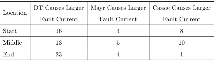
The number of times each fault model type produced a larger fault current magnitude

at each location is show in Table 5.5. It is clear to see that definite time arc modelling

consistently produces a larger fault current magnitudes. However, as previously indicated

this study will focus on the Mayr and Cassie models as the definite time modelling does not

simulate a change in impedance between the circuit breaker contacts as they part. This

subsequently means that definite time modelling will have a lower fault circuit impedance

that does not change for the entire fault duration; giving a larger fault current magnitude

(52)

[image:52.595.111.488.118.226.2]

5.2 Arc Model 38

Table 5.5: Arc Model Effect On Fault Current Magnitude

Location DT Causes Larger

Fault Current

Mayr Causes Larger

Fault Current

Cassie Causes Larger

Fault Current

Start 16 4 8

Middle 13 5 10

End 23 4 1

When considering the Mayr and Cassie arc models only, Table 5.6 indicates the number

of times each model produced a larger fault current magnitude at each location. It is

interesting to note that the fault arc models appear to respond differently at each of

the three faulted locations. The start of the line produces a relatively even distribution

between the Mayr and Cassie model. The middle of the line shows the Cassie model

producing larger fault magnitudes; conversely the end of the line shows the Mayr model

[image:52.595.160.436.424.528.2]

producing larger fault magnitudes.

Table 5.6: Mayr vs. Cassie Effect On Fault Current Mag

Circuit breaker simulated operation & behaviour under faulted power system conditions

University of Southern Queensland

Abstract

Certification of Dissertation

Acknowledgments

Contents

List of Figures

List of Tables

Chapter 1

Objectives

Resource Requirements

Chapter 2

Technical Background

P = EAED

Fault Data

Chapter Summary

Chapter 3

Circuit Breaker Characteristics

Transmission Line Characteristics

Network Fault Levels

Network Loading Effects

VREC =VLN

Definite Maximum Fault Time

Arc Models

Arc Conductance

Fault Impedance

Chapter Summary

Chapter 4

Simulink Model Introduction

Definite Maximum Fault Time

Arc Resistance & Conductance Calculation

Mayr Arc Model

Cassie Arc Model

Fault Location

Fault Impedance

Fault Inception Angle

Chapter Summary

Results and Discussion

Results Summary

Arc Model