Calculating positional and survey uncertainty for terrestrial observations

May 2018

C

ALCULATING

P

OSITIONAL

AND

S

URVEY

U

NCERTAINTY

FOR

T

ERRESTRIAL

O

BSERVATIONS

Background

In Queensland the Survey and Mapping Infrastructure Act 2003 gives the Chief Executive of the Department of Natural Resources and Mines and Energy the power to makes standards and guidelines in relation to the performance of cadastral surveys. Two of the standards (3.14.3 and 3.28.1 in the

Cadastral Survey Requirements) rely on the concepts of survey uncertainty (SU), positional uncertainty (PU) and relative uncertainty (RU). SU represents the uncertainty in control mark co-ordinates at the 95% confidence level free from the influence of any imprecision or inaccuracy in the underlying datum realisation. PU is the SU with the addition of the uncertainty in the datum realisation and RU is the uncertainty of the join between two control marks (for more detailed definitions see p5 of the ICSM’s Special Publication 1 (SP1)

https://www.icsm.gov.au/publications/standard-australian-survey-control-network-v21). The

Cadastral Survey Requirements gives clear guidelines as to the calculation and validation of these values when using RTK GNSS observations (see s8.4). The purpose of this paper is to give some background and guidance for calculating uncertainty for terrestrial methods.

Error Propagation

The law of propagation of errors is concerned with the behaviour of random errors propagating through a measurement system.

Linear Problems

When the final value is created by the linear addition of independent measurements the error associated with it takes on the simplest form;

1 2 2 1

( n )

X i

i

 



where σx is the standard deviation of the result and σi are the standard deviations of the n independent

measurements. To be less mathematical the σx is obtained by taking the square root of the sum of the

variances of the individual measurements (for a measurement the standard deviation is the square root of the variance).

Example 1

The total distance A−D and its standard deviation is required. The line was measured in three independent sections as follows:

AB 51.00 m ± 0.05 m

BC 36.50 m ± 0.04 m

CD 26.75 m ± 0.03 m

The total distance of AD = AB + BC + CD

From the law of propagation of errors













2 2 2 2

2

0.05 0.04 0.03 0.005 0.071 AD CD AD A C D AB B               

Uncorrelated Non-Linear Problems

More often than not in surveying individual measurements need to be combined to get the desired parameter. A common example is calculating a horizontal distance from a slope distance and vertical circle reading.

sin

h s  (2)

where h is the horizontal distance, s measured slope distance and  is the measured zenith distance (if using the vertical angle then the trig function changes to cos). Rather than the simple addition from Example 1 the measurements are being combine non-linearly.

In general terms, if y represents a quantity computed from several measurements (random variables) represented by x₁, x₂, ..., x_n in a non-linear function y = f (x₁, x₂, ..., x_n) and if σ₁, σ₂, ..., σ_n represent the standard deviations of the measurements x₁, x₂, ..., x_n which are assumed to be independent.

Then, σ_y is computed by

2 2 2 1 i n y x i i y x      _{ }    



A horizontal distance needs to be calculated from a slope distance is s = 100.00 m with σ_s = 0.05 m and β = 85°00' with σ_β = 00°30'. Compute h and σ_h. (Assume s and β to be uncorrelated.)



 

 



2 2 2

2

2 2 2 2

sin (100.00)(0.996195) 99.6195 m

30 60

sin 0.05 m

206265 0 cos 0.0083 .091 m h s h h h s s h s         _{ }  _{ }                     _{  }   

General Non-Linear Problems

In the previous section we assumed that the measurements were independent. It is clear that when two different parameters are calculated with the same raw measurements then the results, and the error estimates will have some relationship to each other. For our purposes the obvious case is the

calculation of co-ordinates from a radiation. It is clear that the Easting and Northing co-ordinates are calculated from the same distance and bearing observations so that errors in each of those

observations will ‘show up’ in both co-ordinates but in a different way. Because they are connected in this way the two co-ordinates of a pair co-vary and so do the errors. So rather than talking about the variance we have to expand it to a 2 x 2 matrix called the variance co-variance matrix (VCV).

2 2

T

E EN

NE N

VCV   J J

 

 

_{ } 

  (4)

where the variances of the co-ordinate values are as before σ_EN = σ_NE is the covariance,  is a matrix of variances and J is the Jacobian matrix of the partial derivatives.

In the case of the two dimensional co-ordinate pair the change in the co-ordinate values from a radiation are given as

sin cos E h N h    

  (5)

where h is the horizontal distance andθ is the bearing. In this case the measurement of distance and bearing are independent so the variance matrix is only diagonal.

2

2

0 0

h

E E N N

h h h

VCV

N N E N

h                             _{ }    _{ }   _{ }              (6)

Combining Eqns (4) - (6)

2 2

2 2

sin cos 0 sin cos

cos sin 0 cos sin

h E EN

NE N

h VCV

h _ h h

                      _{   }_{ }  

      (7)

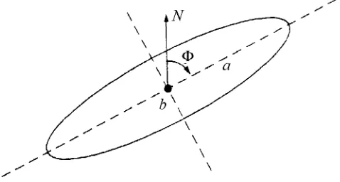
While the variances and covariances are useful measures of the precision of the co-ordinates it can be proved that the errors are more correctly represented by an ellipse which is based on the geometry of the survey observation rather than the co-ordinate system.

Figure 1 The error ellipse parameters

This is of far more use to surveyors so the next step is to determine the size of the semi-major and semi-minor axes, and the orientation of the ellipse from the VCV for the co-ordinate pair.

Without proof, the size of the major and minor axes are calculated from eigenvalues of the square matrix. a ₁andb ₂ where₁and₂are the eigenvalues.(The eigenvalues are those

numbers that need to be subtracted from the variances so that the determinant of the VCV equals zero) For the 2 x 2 matrix eigenvalues are given by the following formula, where λ₁ is the maximum value which will give the semi-major axis of the ellipse.





1 1 ( ) 4

2 E N E N EN

a            (8)





2 1 ( ) 4

2 E N E N EN

b            (9)

The orientation of the major axis is given by the bearing Φ, which can be determined using the formulae:

2 2

2

tan 2 EN

N E

  

   (10)

The correct value of 2Φ is selected such that sin 2Φ has the same sign as σ_EN and cos 2Φ has the same sign as (  2N 2E).

Example 3

Compute the error ellipse for a single radiation. The horizontal distance is h = 200.0 with σh = 0.004

2 2

2

2

6 6

sin cos 0 sin cos

cos sin 0 cos sin

0.004 0

0.258819 193.18517 0.258819 0.965926

3

0.965926 51.76381 0 193.18517 51.76381

206265 8.97x10 1.88x10

h h

VCV

h _ h h

                  _{   }               _     _   _{   }     

 _{6 5}

1.88x10 1.55x10

      0.00296 0.00394 E N    

2 2 2 2 2 2

1

(

(

)

4

) 0.004

2

a























2 2 2 2 2 2

1

(

(

)

4

0.0029

2

b























2 2

2

tan 2 0.577655

2 30.0 15 EN N E           

Converting Error Ellipses to SU

ICSM’s Special Publication 1 (SP1) provides a method to convert an error ellipse to a circular confidence region. The SU can be calculated from the standard (1 sigma) error ellipse using;

2 3

* 1.960798 0.004071[ b 0.114276 b 0.37165 b ]

SU a

a a a

   

   

  

 

  _{ }  

   (11)

where a and b are the semi-major and semi-mior axes as before.

Example 4

Using the result of Example 3 calculate the SU for that point. 0.004 0.0029 0.725 a b b a          2 3

0.004 * 1.960798 0.004071 0.725 0.114276 0.725 0.37165 0.725 ] 0.0086

[

SU      

The Effect of Bearing on the Error Ellipse

The previous calculations are clear cumbersome to perform for every line of the traverse. However if we examine the effect of the radiation bearing on the variances and SU we can take advantage of symmetry. The Table below shows the result of the previous calculations if we hold all measurements constant but just vary the bearing of the radiation.

Table 1 Table showing the variation in the error ellipse with the change in radiation bearing

Bearing (°)

σ

σ

0 0.0029 0.0040 0.004 0.0029 0

10 0.0029 0.0040 0.004 0.0029 10

20 0.0031 0.0039 0.004 0.0029 20

30 0.0032 0.0038 0.004 0.0029 30

40 0.0034 0.0036 0.004 0.0029 40

50 0.0036 0.0034 0.004 0.0029 50

60 0.0038 0.0032 0.004 0.0029 60

70 0.0039 0.0031 0.004 0.0029 70

80 0.0040 0.0029 0.004 0.0029 80

90 0.0040 0.0029 0.004 0.0029 90

The table shows that for a single radiation the standard deviations on the co-ordinates vary with the radiation bearing but the ellipse maintains the same shape and merely rotates. This is a useful result as only the semi-major and semi-minor axes are used to calculate SU and they are invariant with the bearing.

Simplified SU Calculation

Figure 2 shows the relationship between the bearing and distance uncertainties and the resultant error ellipse.

A simplified calculation for SU for a single radiation is to calculate the axes using;









max , tan min , tan

h

h

a h

b h





 

 



 (12)

Figure 2 Figure showing the relationship between the error ellipse axes and radiation observations.

Example 5

Compute the error SU for a single radiation using the simplified method. The horizontal distance is h = 200.0 with σh = 0.004 m and the bearing θ is 15°00' with σθ =3″

2 3

0.004

tan 200.tan(3") 0.0029 = 0.725

0.004 * 1.960798 0.004071 0.725 0.114276 0.725 0.37165 0.725 ] 0.0086

[

h h

a b SU



 



 

     

      



Calculating PU for an Open Traverse

For an open traverse however each leg of the traverse can be dealt with as if it is independent so the propagation of the error is as simple as Eqn. (1).

Example 6

Starting from PM123456 with a PU of 0.011 you traverse to a new point B via two traverse legs. PM-A θ is 65°00' h = 92.5 m, A-B θ is 142°00' h =60.35 m with σh = 0.003 m + 2ppm and with standard

deviation of a single pointing σp 5″. The centring accuracy is σc = 0.002 m Compute PU of B.

(Reading two faces)

The bearing is the difference between two pointings of the total station so it is necessary to calculate the standard deviation of the bearing using Eqn. (1). The standard deviation of a mean measurement is

x s s

n

 where s is the standard deviation of the sample and n is the number of observations that are being meaned. In our case the n = 2 as two faces are being read and we use the instrument stated standard deviation for a single pointing.

2 2 ₂ 2

5 2

p p p

p n



  

      

Next calculate the SU for each leg.

Bearing (°) Distance

σ

σ

65 92.5 0.0032 0.0022 0.0068

142 60.35 0.0031 0.0015 0.0063





2 2 2 2 2

1

2 2 2 2

2 0.011 0.0068 0.0063 2 0.002 0.0147

n

B i PM PM A A B c

i

PU  PU SU _ SU _ 



    

   





You will note that we have assumed that forced centring is being used so there are only two centring variances and the initial backsight is far enough away that its centring error does not contribute to the bearing uncertainty. If forced centring was not being used then there would have been four centring errors.

Acknowledgement