City, University of London Institutional Repository
Citation
:
Papoutsakis, A., Sazhin, S., Begg, S., Danaila, I. and Luddens, F. (2018). An
efficient Adaptive Mesh Refinement (AMR) algorithm for the Discontinuous Galerkin method:
Applications for the computation of compressible two-phase flows. Journal of Computational
Physics, 363, pp. 399-427. doi: 10.1016/j.jcp.2018.02.048
This is the accepted version of the paper.
This version of the publication may differ from the final published
version.
Permanent repository link:
http://openaccess.city.ac.uk/20657/
Link to published version
:
http://dx.doi.org/10.1016/j.jcp.2018.02.048
Copyright and reuse:
City Research Online aims to make research
outputs of City, University of London available to a wider audience.
Copyright and Moral Rights remain with the author(s) and/or copyright
holders. URLs from City Research Online may be freely distributed and
linked to.
An e
ffi
cient Adaptive Mesh Refinement (AMR) algorithm for the Discontinuous
Galerkin method: applications for the computation of compressible two-phase
flows
Andreas Papoutsakisa,∗, Sergei S. Sazhina, Steven Begga, Ionut Danailab, Francky Luddensb
aAdvanced Engineering Centre, School of Computing, Engineering and Mathematics, University of Brighton, Brighton, BN24GJ, UK bLaboratoire de Math´ematiques Rapha¨el Salem, Universit´e de Rouen Normandie, F-76801, Saint- ´Etienne-du-Rouvray, France
Abstract
We present an Adaptive Mesh Refinement (AMR) method suitable for hybrid unstructured meshes that allows for local refinement and de-refinement of the computational grid during the evolution of the flow. The adaptive imple-mentation of the Discontinuous Galerkin (DG) method introduced in this work (ForestDG) is based on a topological representation of the computational mesh by a hierarchical structure consisting of oct- quad- and binary trees. Adap-tive mesh refinement (h-refinement) enables us to increase the spatial resolution of the computational mesh in the vicinity of the points of interest such as interfaces, geometrical features, or flow discontinuities. The local increase in the expansion order (p-refinement) at areas of high strain rates or vorticity magnitude results in an increase of the order of accuracy in the region of shear layers and vortices.
A graph of unitarian-trees, representing hexahedral, prismatic and tetrahedral elements is used for the represen-tation of the initial domain. The ancestral elements of the mesh can be split into self-similar elements allowing each tree to grow branches to an arbitrary level of refinement. The connectivity of the elements, their genealogy and their partitioning are described by linked lists of pointers. An explicit calculation of these relations, presented in this pa-per, facilitates the on-the-fly splitting, merging and repartitioning of the computational mesh by rearranging the links of each node of the tree with a minimal computational overhead. The modal basis used in the DG implementation facilitates the mapping of the fluxes across the non conformal faces.
The AMR methodology is presented and assessed using a series of inviscid and viscous test cases. Also, the AMR methodology is used for the modelling of the interaction between droplets and the carrier phase in a two-phase flow. This approach is applied to the analysis of a spray injected into a chamber of quiescent air, using the Eulerian-Lagrangian approach. This enables us to refine the computational mesh in the vicinity of the droplet parcels and accurately resolve the coupling between the two phases.
Keywords: Droplets, Sprays, Vortex Rings, Discontinuous Galerkin, Adaptive Mesh Refinement
1. Introduction
The variety of different spatial scales observed in compressible, dispersed, multiphase flows reflects the more general problem of the interaction between the micro- and the macro-scales in fluid mechanics [1]. There is a signif-icant number of examples where the physical flow problem is the result of a closely-binded synergy of phenomena occurring at different scales [2, 3, 4]. In compressible, dispersed, multiphase flows we observe the interaction of the macroscopic flow in the following ways:
i) with refined structures due to compressibility (e.g. shock and acoustic waves [5, 6], thermal effects and chemical reaction regions [7], [8], [9]),
ii) with vortical structures [10], and
∗
iii) with dispersed micro-scale droplets and particles [11], moving walls and detailed solid structures [12] or solidification interfaces[13].
Due to the complexity of these interactions, we need to resolve all scales of the problem. Small scale features in a complex flow are not knowna-prioriand can vary in time. To fully resolve a complex flow, fine resolution is required throughout the computational domain. This fine resolution allows us to describe fine structures and features of the flow.
Adaptive Mesh Refinement (AMR) addresses the problem of resolving this wide range of scales by focusing the discretisation resolution in the proximity of the fine structures. The Finite Element (FEM) framework [14] for the solution of PDE’s gives us two options to enhance the spatial resolution (and accuracy) of discretisation. Firstly, this can be achieved by increasing the number of basis functions used for the discretisation of the field variables, resulting in an increase of the degrees of freedom within the element and the order of accuracy of the discretisation (i.e.p-type refinement) [15, 16]. Secondly, this can be achieved by local increase of mesh resolution (i.e. h-type refinement), a strategy which is also relevant to the Finite Volume (FV) [17, 18] and Finite Differences [5] framework. Also, a combination of both approaches (i.e.h/p-type refinement) can also be applied [19, 20].
By localising the discretisation resolution, the desirable resolution can be achieved with minimal increase of the size of the problem. H-type refinement results in the re-arrangement of the computational grid. This can be achieved either by relocating the nodes of the mesh [7, 21, 22, 23] or by splitting existing elements in smaller ones [24, 19, 25, 26]. The relocation of the mesh vertices allows us to retain the connectivity topology but eventually leads to highly anisotropic elements [23]. This approach allows us to focus on areas of interest without increasing the total number of degrees of freedom. An alternative approach is to start from the finest resolution and locally coarsen the mesh and/or decrease the original order of accuracy [20]. This is achieved by agglomeration based, adaptive implementations. One of the advantages of this approach is that the finest grid is accurately prescribed. Thus, it can deal with highly anisotropic meshes appearing at the highest refinement level in high Reynolds viscous simulations [27]. Furthermore, agglomeration techniques, being inherently related to multigrid methods, can lead to major convergence performance benefits that stem from multigrid solvers [28, 29].
Splitting of cells may be achieved by retaining the existing faces of the mesh [25, 30] and introducing verticies inside the elements, or by introducing new vertices leading to non-conformalities [31, 19]. The second approach to cell splitting results in an increase in the total number of elements and the re-arrangement of the inter-element connectivity relationships. This method of cell-splitting in AMR requires a versatile data structure. According to [32], approaches to cell splitting in AMR can be classified into three distinct categories: block structured AMR (SAMR), unstructured AMR (UAMR) and tree AMR (TAMR). SAMR utilises the regular mapping of the structured grids at the expense of numerical complexity. UAMR, on the other hand, offers the flexibility of unstructured meshes through the use of an adjacency graph. The TAMR approach, introduced in [33] and [34, 32, 13] for the4estcode, uses a forest of trees structure for the description of the locally refined mesh and thus creates an internal mapping [32] for the derivation of the connectivity relations of the refined grid. In the category of unstructured split cell FEM solvers, thedeal-II FEMlibrary offers an object oriented data structure [35] for AMR on hexahedral elements, and has been widely used for the solution of the Navier-Stokes equations [36]. TheLibmesh[37] FEM library also provides a versatile data structure for the implementation of adaptive oct-tree refinement on triangular and prismatic elements for numerical simulations in hybrid unstructured meshes. We use the forest of trees structure to describe the topology of a split-cell refined hybrid unstructured mesh. The connectivity graph relations of the refined grid are calculated based on the varying relative relations of the ancestral elements and the predefined internal structured mapping in the tree. The versatility of pre-defined tree split structures (e.g. oct- quad- and binary trees) has made them applicable to a wide range of problems [4].
The Discontinuous Galerkin method [38, 39, 40, 41] combines high order accuracy with the ability to handle complex geometries described by hybrid unstructured meshes. The computational efficiency of this method (alongside the spectral volume [40, 42] and spectral difference [40, 43, 44] methods), however, is generally believed to be inferior to more commonly used methods, such as the Finite Differences (FD) and Finite Volume (FV) [45, 46] methods.
cells. The DG method provides a compact, discretisation stencil, where the inviscid and viscous fluxes are calculated from the solution within the element and only the surface integrals, at the adjacent neighbouring faces, are taken into account. Oct-tree based refinement has been associated with the generation of spurious shocks, in Finite Difference AMR implementations [4, 50, 51]. However, the compact, discretisation stencil used in the DG method, as well as the treatment of the non-conformal faces as faces of a polyhedral element, results in the elimination of spurious shocks and oscillations [52, 53]. Moreover, accurate integration of the inviscid fluxes in non-conformal faces is known to remove the occurrence of spurious shocks in compressible simulations using Finite Volume [54] and Finite Difference [55] approaches. The compatibility of the DG discretisation with adapted unstructured meshes and the improvement of the computational efficiency of the DG method due to AMR leads to a powerful combination for solving complex flows.
The identification of the fine structures which drives AMR is primarily based on the characteristics of the resolved flow field. The gradients of the flow field, quantified by the magnitude of the vorticity or the strain tensor, show the regions of potential flow instabilities [56, 10]. Also, the local mesh size [57], and the density gradients [8] can serve as criteria to identify shocks. The geometrical features of the flow field, e.g. the solid boundaries [13, 12] or the location of inertia particles [17, 11] can also be used as AMR criteria. Refinement criteria based on the estimation of expected spatial errors have been suggested in [58, 59]. These are used to drive AMR adaptation for unsteady problems. A
posteriorierror estimate techniques [52, 53] are based on the identification of the spatial error distribution. This
approach results in a refinement strategy that optimises the efficiency of the solution and accuracy of the refined discretisation [60]. Validation of simple gradient based criteria, as reasonable choices for the indication of regions to be refined, can be based on the analyses, using error estimate techniques [61].
In this paper a new mesh adaptive method associated with the Discontinuous Galerkin methodology is suggested. This approach allows on the fly localh/p-type refinement and de-refinement of the computational mesh [8]. An efficient algorithm for the implementation ofh/p-type refinement is described and it is applied to the design of a new computational code (ForestDG). ForestDG is based on modal, hierarchical basis, as described in [62, 63] for the case of conforming hybrid meshes. The use of modal basis in best suited forh/p-type refinement [64, 65]. In contrast to nodal basis, modal basis are evaluated in the computational space, thus allowing a simpler evaluation of the volume integrals and fluxes across non-conforming element faces. We show that a hierarchical representation of a forest of binary, quad- and oct- trees is highly efficient and we introduce a unified methodology for the efficient splitting, merging and repartitioning of hexahedral, prismatic and tetrahedral elements. Furthermore, the accuracy and performance of the new code are assessed. Finally, the ability to capture discontinuities, moving vortical structures and the dispersed phase in multiphase flows, is demonstrated for several examples.
In Section 2 we present the general formulation of the governing equations for the modelling of mass, momentum and energy conservation of a compressible flow. In Section 3 the discretisation of these equations in the DG framework is described. In Section 4 we introduce the forest structure for the representation of an adaptive unstructured mesh. In Section 5 we describe the splitting and merging techniques occurring during the adaptation of the computational grid to the flow field solution. In Section 6 we describe the algorithm introduced for the efficient assignment of the connectivity problem during the adaptation of the grid. In Section 7 we present a series of test cases for subsonic and supersonic configurations where we assess the accuracy of the algorithm, the efficiency of the proposed method and the computational performance of the code. In Section 8 we demonstrate the capabilities of the code to capture moving structures for the problem of an inviscid supersonic flow around a cylinder in a duct. In Section 9 we demonstrate the resolution of the flow discontinuities and reaction regions arising from the interaction of the oblique shocks in the case of a hypersonic flow around a double cone configuration. In Section 10 we use the solver introduced in this paper for the solution of a dispersed multiphase flow arising during spray injection of gasoline fuel.
2. Governing equations
The method presented here is developed for the general case of viscous compressible flows. The basic set of governing equations correspond to the flow field of a compressible viscous fluid described by the state vectorU(x,t) in Eulerian coordinates, which contains the values of densityρ, momentumρuand energy ρeat each position of the computational domainx at timet. Depending on the case modelled, the state vectorU(x,t) can be extended to include the vibrational energyevneeded for the Park’s model [66] for air dissociation simulations, the species specific
compressible turbulent dispersed two phase flow simulations, the carrier fluid phase is modelled as an Eulerian flow fieldU(x,t) and the droplets are suspended in the carrier gas phase and are modelled using the Lagrangian approach.
Sub-grid turbulent fluctuations are modelled using the one-equation Spalart-Allmaras (SA) model [67], leading to a Detached Eddy Simulation (DES) [68, 69] approach. The SA model offers an alternative to the standard LES models, that is not dependent on the filter width∆. For the AMR methodology presented in our paper, the cell size changes substantially in space thus making the standard LES models inapplicable. Furthermore, in the spray injection case investigated in our paper, the Spalart-Allmaras model accounts for the effect of the cylinder head wall where a strong recirculation region and detachment of the boundary layer is observed [70].
The Favre averaging operator (e·) = ρ(·)/ρ is used for the separation of the small turbulent fluctuations from
the large ones. The state vector for the Favre averaged velocity u and specific energy e is defined as eU(x,t) =
(ρ, ρeu1, ρeu2, ρeu3, ρee). The conservation of mass, momentum and energy provides the set of the governing equations
for the turbulent compressible flow of the carrier phase. The strong conservative form forUecan be presented as [71]:
∂eU
dt +∇ ·finv
e
U− 1
Re∇ ·fvis
e
U,eΘ
=wd
e
U , (1)
e
Θ=∇fauxUe
, (2)
wherewdis the vector of the source terms stemming from the two way coupling for the momentum and energy transfer
between the carrier and the discrete phase,finvis the 5×3 tensor of the inviscid fluxes andfvisis the 5×3 tensor for
the viscous fluxes, defined as:
finv=
ρeuj ρeuieuj+pδi,j
(ρee+p)euj
, fvis=
0 2 (µ+µt)S∗i,j
2 (µ+µt)euiS ∗
i,j−eq
, wd =−
0
ndfdi
ndfdjeuj
, faux=
" eui
ee #
, (3)
Si j∗ = 12
∂
euj
∂xi +
∂eui
∂xj
−13δi j∂euk
∂xk is the traceless rate of strain tensor related to the viscous stress tensorτi j =2µS ∗
i j, the
non-dimensional local viscosityµis normalised by the dynamic viscosity at the reference temperature. Fluxeqis the summation of the translational, rotational and vibrational heat fluxes which are assumed to be in equilibrium. In this case the heat flux is related to the temperature gradienteq=−κ∇ ·T whereκ=Pr(µ+µt) is the thermal conductivity
of the fluid. For low speed supersonic and subsonic simulations the value of the Prandtl number for the air is taken equal to 0.76.
The auxiliary state vectorΘecontains the spatial gradients of the 4×1 auxiliary fluxfauxfor the diffusive
com-ponents of the state vectorUeas defined in Equation (2). The viscous fluxesfvisare evaluated fromΘe. The auxiliary
variables vectorΘeis discretised separately resulting in three equations for each of the four diffusive components of
the state vector. As a result, Equation (2) is solved at the same accuracy with the state variables. Equations (1) and (2) comprise the coupled formulation of the governing equations foreX=
h e
U,Θe i
for a turbulent compressible two phase flow.
The contribution of sub-grid turbulence scales, not accounted by the spatially filtered state vector, is taken into account by the turbulent dimensionless viscosity termµtin the definition of the viscous fluxes in Equation (3). In the
Spalart-Allmaras modelµtis estimated by the variable ˆνtas:
µt=ρνtˆ fu1, (4)
where ˆνt is calculated by the integration of the equation for the turbulent viscosityνt used in the Spalart-Allmaras
model:
∂ρνˆt
∂t +
∂ρeujνˆt ∂xj
=ρcb1(1− ft2) ˆSνˆt−ρ
cw1fw−
cb1
κ2 ft2
νˆ
t
d
!2
+σ1 "∂∂
xj ρcb2
∂νˆt ∂xi
∂νˆt ∂xi
#
− 1 σ
∂ρ ∂xi
∂νˆt ∂xi
. (5)
The constants and parameters fu1,cb1, ft2,cw1, fw,cb1,κ, ft2,σandcb2are provided by the model described in [67] and its modified version for the areas of negative viscosity as described in [72]. Parameter ˆS is related to the rate
of strain tensor|Sfi j|=
q
2eSi jeSi jand the vorticity magnitude of the resolved field, acting as a source term for turbulent
The transport equations of each speciessis expressed in terms of the conservation of densityρs =ρYs of each
species as:
∂ρYs
∂t +∇ ·(ρYsu)=−∇ ·
ρsvd s
+ws, (6)
whereYs is the mixture fraction of a species s, vds = (uds,vds,wds) is the corresponding diffusion velocity, andws
is the chemical source term [8]. The rates of forward and backward reactions are obtained using the Arrhenius approximation, and the vibration-dissociation model developed by Park [66].
The energy equation for a flow withNsreactive species is modified taking into accounting the total energyeT of
the mixture
∂ρeeT
∂t +∇ ·((ρeeT+p)u)=∇ ·(τ·u)− ∇ ·
˜qt˜qr˜qv− ∇ · s=ns X
s=1
ρshs~vds . (7)
Fluxes ˜qt,˜qr,˜qv are the translational, rotational, and vibrational heat flux vectors, respectively; h
s is the total
specific enthalpy of the speciess. Translational and rotational energies refer to the translational and rotational motions of the molecules, whereas vibrational energy refers to the energy of vibrations of the chemical bonds in polyatomic molecules. In the current work, a simplified form of the energy equation is used. In this equation, the vibrational energy of diatomic species is described by a single vibrational temperature. This allows us to solve the equation for the total vibrational energy of the mixture instead of separate equations for each of the polyatomic species. This equation for the vibrational energy per unit volume is presented as:
∂ρeev
∂t +∇ ·(ρeev˜u)=−∇ ·˜q
v− ∇ · s=Nd
X
s=1
ρsevs~vds . (8)
whereev
sis the vibrational energy per unit mass of speciess,wuis the vibrational energy source term,Ndis the number
of diatomic species in the mixture.
The relation between vibrational energy and vibrational temperatureTvis inferred from the following expression:
ev=
Nd X
s=1
evs= Nd X
s=1
R
Ms
θv s
eθ
v s T v −1
, (9)
whereθv
sis the characteristic temperature of vibration for each diatomic species,Msis the molecular weight, andRis
the ideal gas molar constant.
Although the above equation provides an explicit definition of the vibrational energy it is solved with an iterative method for the calculation of the vibrational temperature from a given vibrational energy. Equation (1) has been non-dimensionalised over the characteristic length of the flow, gas dynamic viscosityµgand gas densityρgat ambient conditions. The Reynolds number of the flow is estimated as Re = ρgcL/µg, where cis the velocity of sound at ambient conditions.
The discrete phase is modelled as parcels of droplets with diametersdd, velocitiesvdand densityρd. The effect of
the dispersed phase on the energy and momentum of the carrier phase is modelled as the source termwd in Equation
(3).ndis the droplet number density. The term fdiin Equation (3) is the force acting on each individual droplet in the
parcel. Assuming a steady Stokes flow, the expression for the drag force can be presented as:
ndfd =
3ndcDπddµ
Re eu−vd
, (10)
where,cD=
1+0.16667Re2d/3is the correction for the Stokes force for large droplet Reynolds numbers (Red >1).
The trajectories of droplets are described by the following equations:
dxd
3. Discretisation of the equations
We consider the discretisation of the computational domainΩintoNelementsEm(Ω =∪Em). A weak formulation
of the governing equations is derived by multiplying the conservative form of these equations with a test function
w(x) and integrating them over the element. In the Galerkin context, the test function is taken from the same set of polynomial basis functions as used for the interpolation of the state vectoreUand the extended state vectoreX=
h e
U,eΘ i
. The interpolated distributionXm
h forXeis defined for each elementEmas the weighted sum ofNp polynomial basis
functions:
Xmh = Np X
i=1
cmi(t)bi(x),form=1,Np, (12)
where p is the maximum degree of the basis functions. A similar expansion is assumed forUm h andΘ
m
h. In this
expansion, the solution coefficients ci(t) are the degrees of freedom. bi(x) is the tensor product of the Legendre
polynomial basis functions in the three spatial dimensions. The integral formulation of Equations (1) is expressed as:
Z
Em
bi ∂Um
h
∂t dE+
I
Sm
bifXmh·ndS −
Z
Em
∇bi·f
XmhdE=
Z
Em
biwmddE for i=1,Np, m=1,N, (13)
Z
Em
biΘmhdE =
I
Sm
bifauxUmh·ndS −
Z
Em
∇bi·faux
UmhdE for i=1,Np, m=1,N, (14)
providing a set ofNp×Nequations forcmi (t).
The surface integrals are defined on the surface of the elementSm=∂Emwithndefined as the outward normal unit
vector. In the weak formulation presented in Equation (13), the fluxfrepresents both the viscous and inviscid fluxes in Equation (1) asf=finv−(1/Re)fvis; the fluxfauxwas defined in Equation (3). In the DG context we do not require the
continuity of the interpolated variables across the element faces. Thus, the values ofUm h andΘ
m
h on the facesSmare
defined twice. The conservation of fluxes at the boundaries of the elements infers from the approach to the evaluation of the surface integrals used in our analysis. In the Local Lax-Friedrichs (LLF) scheme for the evaluation of viscous fluxes, the signs of surface sides of the elements (referred to as minus (−) or plus (+)) are introduced.
Calculating the fluxes from one of the two sides for the adjoin elements guarantees the conservation properties of the scheme. Specifically, for the LLF scheme the surface integrals forfvisandfauxin Equation (1) are evaluated from the opposite sides as:
fvis=fvis
U−mh,Θ−mh, faux=faux
U+mh . (15)
The inviscid fluxfinvis evaluated from the mean value of the variables on the two face sidesnUmho, where an artificial diffusion term, proportional to the jump of the fluxes on the bounding surface [[Umh]], is introduced via the equation:
finv=finvnUmho+λi
2[[U
m
h]], (16)
where, in the LLF scheme,λi=max
|finv0 (Ui)|
is the maximum absolute eigenvalue of the inviscid flux at the specific position of the interface (Local).
The volume and surface integrals in Equations (13) and (14) are defined in the physical space. The integrals are evaluated in the transformed domain for the computational space elements using the Gauss-Legendre quadrature rule and the Jacobian of the transformation [14]. Using the transformations described by Equations (A.1) to (A.3) the physical coordinates (x)Em for each element of the discretisationE
m are transformed to a computational space Ωmwith coordinatesη1, η2 andη3. This transformation maps any hexahedral prismatic or tetrahedral elementEm
to a cube withηi ∈ [−1,1] using collapsed coordinates [14]. Introducing the Jacobian of the transformation to the computational space, the volume integrals of a field, expanded as in (12), is evaluated as:
Z
Em
bi(x) Np X
j=1
cmj(t)bj(x)dE=
Z
Ωm
bi(x) Np X
j=1
The above integral is now defined in the standard computational space and is calculated by evaluating the integral function onNqp selected quadrature points ofΩm: ~ηi,j,k =~ηiq. Finally, the integral on the right hand side of (17) is
approximated by the Gauss-Legendre quadrature rule with weightsW(~η) pre-calculated at~ηiqas:
Z
Ωm
bi(x) Np X
j=1
cmj(t)bj(η˜)J(~η)dΩ = Neq X
iq=0
Np X
j=1
bi(~ηiq)cmj(t)bj(~η)J(~η)W(~η). (18)
Similarly, surface integrals in Equations (13,14) are calculated on quadrature points~ηiq,f defined at each active
face of the computational domainΩ. Although the AMR methodology introduced here presents shock capturing characteristics by enhancing the resolution of discontinuities arising in compressible flows, a unified limiting approach is needed to detect and smooth sharp gradients. The unified Total Variation Bounded (TVB) limiter proposed by Shu and Cockburn [73] for capturing discontinuities with high order (p1 and higher) DG discretisation, is used in our analysis. Although the AMR presents shock capturing characteristics by enhancing the resolution of discontinuities arising in compressible flows, a unified limiting approach is needed to detect and smooth sharp gradients. The unified TVB limiting approach [73], described in [62, 63] for 3D solutions and its extension [8] to the set of equations provided by the Park’s model, is applied in the space of characteristics, as described in [74]. In the AMR methodology introduced here, the detection of discontinuities accounts for the distribution of the solution of non-conforming adjoint faces.
4. Mesh representation
Unstructured, conforming grids are represented using a finite serial addressing of the cells with each cell deter-mined by the addresses of its vertices. The connectivity of the cells is defined by appointing the numerical addresses of the neighbouring cells to each face. In our case, the numerical list of the cells is substituted by a hierarchical graph representation of the elements.
The computational domain is descretised intoNancestral elementsEmconstituting the initial coarse unstructured
grid. Any ancestral element can be split into a number of kids of the same type. Any of the resulting siblings can be further split to more kids up to an arbitrary levelL. A kid of a parentPobtains a unique addressAand is assigned an indexiAl = ithat identifies it as the ith element of its parent treePat levell. The address ofAis related to the address of the parent Pas A = {P,iAl}. Expanding the genealogy of the parent element P, the kidAis defined as
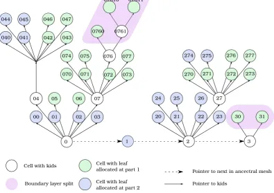
A={Em,i1A,iA2, . . . ,iAl}. A parent shares the same indices with its kidsiA0,iA1, . . . ,iAl−1up to the levell−1. The index of any tree at the zero level is the index of the initial ancestral meshiA0 =m. Thus, each element obtains a unique address that is traced back to the ancestral element. The topology created by the hierarchical relations of the resulting elements forms a forest of nodes.
4.1. Forest and Tree structures
The address Aof each element is a pointer to the tree node data structure shown in Figure 1. The pointers A
for all the trees of the domain are stored in the forest data structure. An example of a developed forest is shown in Figure 2. Each node, referred to as tree node, contains all the pointers needed to define the computational element. The most important pointers contained in the tree node structure are the pointers to the parent nodeP, to the lowest level ancestorEm, to the previous tree, to the next tree and to the neighbours for each face of the element. Also, the
ParentT ree
T ree
PreviousT ree NextT ree
AncestorT ree
Local faces Local nodes Keens [f]
Neigs [f]
Leaf
Solution VectorX Children [i]
[image:9.595.214.385.107.270.2]Parameters
Figure 1: The tree node data structure.
scheme of the remaining nodes. The connectivity pointers and the linked lists for accessing the nodes are cut and re-stitched to the new topology, without altering the addressing of the parts of the mesh that are not affected by the new topology, as shown in Figure 3 (Right).
01
00 02 03
04 05 06 07
070 071
074 075
040 041 042 043
044 045 046 047
21
20 22 23
24 25 26 27
271 272 273
274 275 276 277
30 31
07610 07611
Cell with kids
Boundary layer split
Cell with leaf allocated at part 1
Cell with leaf allocated at part 2
Pointer to next in ancectral mesh
Pointer to kids 0
072 073
076 077
0760 0761
2
1 3
270
Figure 2: An example of a forest of oct-trees representing a three dimensional adapted topology.
[image:9.595.100.496.365.644.2]data objects are de-allocated and are replaced by the pointers to the kids.
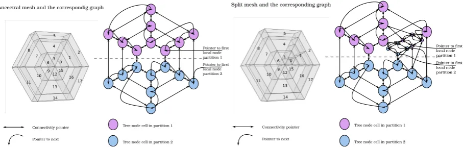
4.2. Domain decomposition
Connectivity pointer
Tree node cell in partition 2
Ancectral mesh and the correspondig graph
Pointer to first local node partition 1 Pointer to first local node partition 2
Pointer to next
Tree node cell in partition 1
0 1
2 3 4 5
6 7 8
9 10 11
12
13
14 15
16 17
Connectivity pointer
Tree node cell in partition 2
Split mesh and the corresponding graph
Pointer to first local node partition 1 Pointer to first local node partition 2
Pointer to next
Tree node cell in partition 1
0 1
2 3 4 5
6 7 8
9 10 11
12
13
14 15
[image:10.595.72.526.161.306.2]16 17
Figure 3:Left:An example of hybrid unstructured mesh and the corresponding graph.Right:Prismatic and hexahedral cells are split into four
cells; the nodes of the adapted mesh are repartitioned by introducing the new nodes to the local element lists and the connectivity pointers are re-defined.
In ForestDG, the graph representation of the computational domain, shown in Figure 3, is fed into the METIS [75] graph domain decomposition library which furnishes an optimised partitioning of the domain. For each partition, a node is assigned as the local first node of the graph defined by the pointerforest->next. The rest of the nodes are accessed iteratively by assigning acrnt->nextpointer to the next node in the list as shown in Figure 3 (Left). During a simulation, the graph is repartitioned resulting in a balanced computational load along the processes, as shown later in Figure 6 for a case of three levels of refinement of an ustructured mesh consisting of tetrahedral elements.
5. Splitting and merging
In the event of splitting a node, a number of new nodes are created. A binary type splitting results in two children, a quad tree type of splitting results in four children, and an oct-tree splitting results in eight children. The parent node is removed from the linked list that controls the access to the cells and is replaced by the children nodes. The next pointers of the linked list are re-stitched in a such way that the parent’s previous tree node now points to the first of the kids created and also the last kid points to the next of the parent, as shown in Figure 3 (Right).
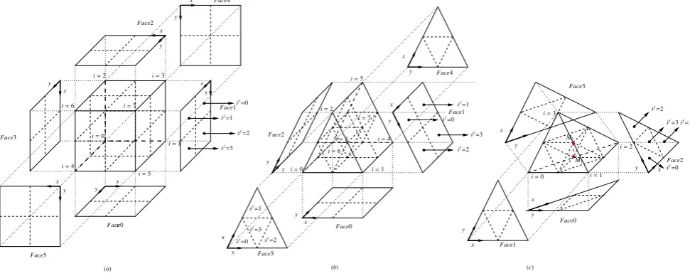
The geometry of the splitting for hexahedral, prismatic and tetrahedral elements is presented in Figure 4. Hex-ahedral elements are split into eight elements which are self similar if the ancestral element has two parallel faces. Four vertices are positioned on the vertices of the higher level cell, three vertices are positioned at the midpoints of the adjacent edges, three vertices are positioned on the centroids of the adjacent faces and a final vertex is positioned at the centroid of the higher level hexahedral, as shown in Figure 4(a).
The numbering of the children follows the numbering of the higher level cell vertices so that the 1st kid is adjacent to the 1st vertex of the cell andith kid is adjacent to theith vertex of the cell. The resulting kids can also be numbered by their positioning in relation to the coordinate system of the element faces adjacent to the kid. For each face f, the kids acquire indexif which is a function of the face index f and the element kid numberi. From the topology
of Figure 4 we can easily construct a simple operator E2F that provides the face index of a kid asif =E2F(iA L,f).
Naturally, E2F is not defined ifiis not adjacent to f.
For prismatic elements, splitting leads to self similar elements (in the case when the ancestral element has two parallel faces) and the cell numbering follows the vertex numbering of the higher level cell. The 7th and 8th children are placed along the core of the prism with reversed orientations, as shown in Figure 4 (b).
i=3
i=0 i=1
i=2
i=4
i=5
if=0
if=1
if=2
if=3
y
y
y
y
y
x
x
x
x x
Face0
Face1
Face2
Face3
Face4
i=7
i=6
if=0
if=1
if=2
if=3
i=1
i=0
i=3
i=2
x y
Face0
Face1
Face2
Face3
x y
x y x
y
if=0
if=1
if=2
if=3
M1
M2
i=5
i=1
x
x x
x
x
x
y y
y y
y
y
Face1
Face0
Face2
Face3
Face4
Face5
if=0
if=1
if=2
if=3
i=3
i=7
i=2
i=6
i=4
i=0
x
[image:11.595.66.552.113.307.2](a) (b) (c)
Figure 4: Topology of oct-tree splitting(a):Hexahedral elements.(b):Prismatic elements.(c):Tetrahedral elements.
the inner octahedron one must choose a splitting plane that lays on the edge connecting the midpoints of two opposite edges of the tetrahedron. One example is the edgeM1,M2shown in Figure 4(c). Choosing the mode for which the distance of the midpointsM1andM2is minimal results in cells with the minimal squewness since this edge is akin to the parent element and remains un-split. The numbering of the resulting elements is shown in the same Figure 4(c).
Given that the size of an element reduces to its half at each split, the level of splitsL, needed to refine an element with a characteristic sizeLto a desirable size`is given by the formula:
L=1.0+log(L/`)
log(2) . (19)
Several quantities can be used as a refinement criterion: density gradients serve as indicators of shocks and vor-ticity (or shear stress magnitude) identifies areas of vortical flow structures. Furthermore, the user can impose a predefined level of refinement based on specific geometrical properties that define certain regions of interest of the flow field.
6. Connectivity assignment
Once the cells are split to the required resolution, the connectivity of the cells needs to be remapped. For the ancestral grid∪Emthe connectivity is resolved by means of tracking the common mesh vertices at the onset of the
simulation. The matching of the common element vertices gives the information on neighbouring cells, neighbouring faces and the orientation of these faces. For the elementEm and at each face f, the pointer Em−> neig[f] to the
neighbouring element En, the pointer Em− > face[f] to the adjacent face fa of the neighbour En and the relative
orientation angleaof the adjacent facesEm−>angl[f] are represented by the following relations:
N(Em,f)=En ,F(Em,f)= fn,A(Em,f)=a . (20)
which must be updated. Here, we present an explicit algorithm that solves the connectivity problem by providing an explicit expression for the three connectivity relations described by Equations (20).
6.1. Connectivity assignment of keen cells
On the first stage, the connectivity is evaluated among the siblings of a split elementP. Given that the elements of the same type, split in the same way are also arranged in the same way, they present a global internal connectivity pattern. This is expressed by the array of keen elementsK. We define a keen element as the neighbour of an element at a specific face if this is a sibling, or the parent of the element if the kid shares the specific face with its parent. Thus, the keen is a neighbour assuming that all the siblings are incubated within the parent cell. This concept leads to an expression of the connectivity which is intrinsic to the specific branch that is being split. This split is neither affected nor affects the connectivity of the neighbouring branches.
For each type of splitting (oct-tree, quad-tree, binary-tree) on each type of tree (hexahedral, prismatic or tetrahe-dral) the connectivity among the siblings remains the same since the siblings are arranged in the same way within a parent. The following array provides the neighbours for theiA
Lth kidA={P,i A
L}ofPwithin an hexahedral element for
each face f:
KAhex[f,iAL]=
{P} {P} {P,0} {P,1} {P} {P} {P,4} {P,5} {P,1} {P} {P,3} {P} {P,5} {P} {P,7} {P} {P,2} {P,3} {P} {P} {P,6} {P,7} {P} {P} {P} {P,0} {P} {P,2} {P} {P,4} {P} {P,6} {P} {P} {P} {P} {P,0} {P,1} {P,2} {P,3} {P,4} {P,5} {P,6} {P,7} {P} {P} {P} {P}
. (21)
As can be seen from the above expression, the keen of each kid{P,iA
L}is its neighbouring sibling{P,j}if the face
f is internal to the parent element. The keen is the parent element itself{P}if f is adjacent to the border of the parent element.
ArrayKA introduces a pre-solved internal connectivity among the siblings. The connectivity outside the parent
will then be evaluated through the connectivity of the parentPand the relative orientations of the ancestral cellEm,
at the second stage. The neighbouring faces between within a branch are evaluated by the arrays FhexA [f,iAL] and
AhexA [f,iAL] which provide the neighbouring face index and the neighbouring face orientation angle, respectively, as:
FhexA [f,iAL]=
0 0 2 2 0 0 2 2 3 1 3 1 3 1 3 1 0 0 2 2 0 0 2 2 3 1 3 1 3 1 3 1 4 4 4 4 5 5 5 5 4 4 4 4 5 5 5 5
, (22) and
AhexA [f,iAL]=0. (23)
The arrays of the keen elements K, the neighbouring faces F and the orientation angles A for prismatic and tetrahedral elements are presented in the Appendix B in Equations (B.1) to (B.6).
6.2. Connectivity assignment of neighbouring cells
In order to locate the direct neighbour of the elementA={Em,i1A,i
A
2, . . . ,i
A
L}at the facef, we evaluate the following
recursive algorithm:
The above algorithm is a recursive evaluation of the keens of the elementAwhich is stored inCwhile the new value is stored inB. At each iteration,Cis a level lower thanB. IfCis at the same level withB, thenBis a direct neighbour ofC = KB[f,ilB]. Hence, BandCare either two neighbouring siblings or two neighbouring ancestral
elementsEm,En. IfBandChave the same level from the first evaluation in line 2, it means thatBis a sibling and a
Rotate Mirror Transform back to Element CS Transform to face CS
Element
i=0 i=1
i=2
i=4 i=6
i=7
FacefA=1
iL=5
i=3
ElementE2FfA(iL) E2FfA=1(iL=5)=3 kid
on the facefAreference
ElementRa E2FfA(iL)
Ra=2
E2FfA=1(iL=5)
=0
ElementMRa E2FfA(iL)
y y
x y
x x
y x
MRa=2
E2FfA=1(iL=5)
=0
ElementF2EfB
MRa
E2FfA(iL)
F2EfB
MRa=2
E2FfA=1(iL=5)
=0
{B}=Khex A [fA,iAL]
Element
Element Element
ElementE2FfA(iL) E2FfA=1(iL=5)=3 kid
on the facefAreference
ElementRa E2FfA(iL)
ElementMRa E2FfA(iL)
x y
y x
ElementF2EfB
MRa
E2FfA(iL)
Element{A}
Element{A} x
y x
y iL=0
i=1 i=2
i=3
i=4 i=5
i=6
i=7 FacefA=3
Ra=0
E2FfA=3(iL=0)
=0 MRa=0
E2FfA=3(iL=0)
=0 F2EfB
MRa=0
E2FfA=3(iL=0)
=0
{C}=Khex B [fA,iAL−1]
[image:13.595.65.536.112.442.2]{C}=Kpri B[fA,iAL−1] {B}=KApri[fA,iAL]
Figure 5:Top:Identifying the neighbouring element of a split element at a hexahedral to prism of oct-tree splitting, incorporating a rectangular
face.Bottom:Identifying the neighbouring element of a split element at a prism to tetrahedron of oct-tree splitting, incorporating a triangular face.
algorithm, we obtain the arrayCwhich is a direct neighbour ofB, andBwhich is an ancestor ofA. At this point, we are certain that the neighbour of the initial arrayAis one of the descendants ofC.
An example of connectivity tracking for two adjacent elements is shown in Figure 5. The keen ofAat the face
f =1 is the elementB. The evaluation of the connectivity of the keens forBwill point to the prismatic elementC, shown on the right side of Figure 5. The elementsBandCcan be two siblings of a parent at a lower level or two ancestral elements of the initial mesh. The elementAis the 5th kid ofB(iAL=5) located at the bottom right corner of
B. Using the operatorE2Ff=1(iAL), the index ofAat the facef isi
f =1. The face is then rotated, using operatorRa, by
the orientation angleaforBandCinferred from (20) or (23). The rotation results in an index of the transformed face
Ra(E2Ff=1(iAL))=0. Finally, given that the faces ofBandCare opposite to each other, the face should be mirrored as
M(Ra(E2F
f=1(iAL)))=0. Thus, the neighbour ofAat f =1 is the kidiLf =0 ofCat face fC. Introducing the reverse
transformationF2Ef(if), the neighbour ofAis provided by the following expression as the jth kid ofC:
jL=F2EfB
MRaE2FfA(iL)
. (24)
The mirror and rotation operators for rectangular and triangular faces are defined as:
Mrec(if)=
0 2 1 3
, Mtri(if)=
0 2 1 3
, Rarec(if)=
1 2 3 0
, Ratri(if)=
Algorithm 1Location of neighbouring ancestorCfor the kidAat the face f.
1: l←Level(A)
2: B←A
3: C←KA[f,iAl]
4: whileLevel(B),Level(C)do
5: B←C
6: C←KB[f,ilB]
7: l←Level(C) (or equivalentl=l−1)
8: end while
In the general case, when the elementsBandCat the intersection of two neighbouring branches are not just one level below, the neighbour ofAis defined as:
N{Em,i1A,iA2, . . . ,iAL},f={C,F2EfB
MRaE2FfA
ilA, . . . , F2EfB
MRaE2FfA
iAL}. (26)
The important advantage of this method is that Equation (26) is explicit and does not involve the connectivity of the neighbouring branch. This equation is based on the connectivity at the closest intersection of the neighbouring branches betweenBandC. In cases of dynamic adaptation, it is never certain that the neighbouring cell actually exists or it is located in the same partition. Formula (26) gives the neighbouring cell address regardless whether the topology of the neighbouring branches has changed or is going to change.
In the case when cellBhas not been refined up to the same levelLof elementA, Formula (26) becomes:
N(A)={C,F2EfB
MRaE2FfA(il)
, . . . , F2EfB
MRaE2FfA(iL−1)
}, (27)
[image:14.595.69.527.413.619.2]whereL−1 is the maximum level which can be reached at the branch ofC.
Figure 6:Left:Domain decomposition for a tetrahedral mesh refined to three levels. Different colours represent the mapping of different partitions.
Right:Pressure distribution for an isentropic vortex projected on a tetrahedral grid.
Furthermore, the address obtained by Equation (26) can be a parent of a cell that has been refined further. In this case, the neighbour pointer ofAat f points to all children ofN(A) located at face fB. Although the splitting/merging
6.3. Solution Projection, Face Fluxes
When a cell is split into a number of kids or when a set of kids merge to their parent, the solution has to be projected from the parent to the kids or visa versa. This is achieved by the Galerkin projection of the solution [76] on the quadrature points of the new element to the basis of the new elements.
An example of Galerkin projection is shown in Figure 6 (Right) where an isentropic vortex field is initially projected on a grid consisting of tetrahedral elements. In Figure 6 (Right) we show the projection of an isentropic vortex field solution from an initial level equal to 2. The solution is projected to the merged tetrahedral elements of level 1 in the outer radius of the vortex and to the split tetrahedral elements with level 3 in the core of the vortex. The mapping of the quadrature points for the new elements in the computational space of the old element is described in Figure 7 (Left).
In the right column of Figure 7 (Left) the topology of the physical space and arrangement of the kids within the physical element are shown for three types of elements discussed above. The physical space is mapped to the computational space shown in the right column of the same figure. Although the arrangement of the kids in the physical space is straightforward and has been described in the previous section, the sub-domain of each kid is mapped to the computational domain of the parents through the transformations (A.1) to (B.3). Assuming thatAandBare two overlapping elements with eitherAcontained inBorBcontained inA, the computational space coordinates ofB
are mapped to the computational coordinates ofAas:
{η1A, η2A, η3A}: xAη1A, η2A, η3A=xBηB1, ηB2, ηB3. (28) In the general case, which includes tetrahedral and prismatic elements, the transformation (28) is not linear. Equa-tion (28) can be solved numerically by introducing the Jacobian∂ηA
i/∂η B
j. All the descendants across the branch on
an ancestral element are split in a similar manner. Thus, this transformation is valid for all the mappings from a parent to its kids and for all the kids to the parent within a branch. For the case of hexahedral elements, the above transformation is linear and the computational space ofBcan be mapped to the computational space ofAas:
ηA
1 =c 1,B
1 η
B
1 +d 1,B, ηA
2 =c 2,B
2 η
B
2 +d 2,B, ηA
3 =c 3,B
3 η
B
3 +d 3,B,
(29)
where coefficientscB anddB depend on the relative position betweenAandBin the computational space. This is
shown for an example of the parent to kid mapping for a hexahedral element at the right column of Figure 7 (Left). Evaluating the current solution on the quadrature points of the new elements, we can project the solution vector on the new elements.
The projection of the solution on kids or parents is also applied for the evaluation of the fluxes for non-conformal faces. Non-conformalities arise due to p-refinement, h-refinement or both as shown in Figure 7 (Right). In [76, 19], a gather operator and a scatter operator are used for the calculation of fluxes on non-conforming meshes. The gather operatorPGiminor is used for evaluating the solution (fluxes) on the major element basis from the minor face basis iminor. The scatter operatorPSiminoris used for evaluating the conserved variables from the major element face to the minor faces basis iminor. The gather and scatter operations are described by the following equations:
f= nmin
X
iminor=1
PGiminorfiminor, and Uiminor=PSiminorU, (30)
wherenminoris the number of minor non-conforming faces. OperatorsPGiminorandPSiminorensure that the flux from the one side of the non-conformal face is equal to the sum of the fluxes to the other side of the non-conformal face and vice versa. This is expressed by the following equations for an arbitrary fieldU:
I
Siminor
Uiminor−UdSiminor=0, for each iminor, and
I
S
U−U˜dS =0, (31)
4
7 8
6 5
1 2
7
5
3
6
7
1 2
3
4
8
5 6
8
1 2
3 4
1 2
3 4
5 6 7 8
ηikid
2
ηikid
1
ηikid
2
ηikid
1
ηikid
2
ηikid
1 3
1 2
6
3
4 5
7 8
1 2
3 4
5 6
7
8
X
+X
+X
−X
−X
+
X
+X
+X
−X
−X
+X
+X
+X
+X
−X
−X
+X
+X
−X
−X
−X
−conforming case
p2:p1
[image:16.595.85.511.108.430.2]1:2
2:1
Figure 7:Left:Transformation from physical to computational space for split hexahedral, prismatic and tetrahedral elements. Blue dots represent
the quadrature points (assumingp1 expansion) on the computational space of the kids. These quadrature points are mapped taking into account the
coordinate transformations for each type of elements to the computational space of their parent . The relative location of the quadrature points is
shown in the right column for each type of element.Right:Types of non-conformalities encountered in h/p adaptive cases. Solid curves indicate
the neighbouring cells, dashed curves indicate the ghost faces on which the solution is projected. In the first step (Scattering), in the case of 2:1 connectivity, for the evaluation of fluxes on the+side the conserved variables from the solution of the−side is projected to the ghost face of the
same level. In the second step (Gathering), in the case of 1:2 connectivity, for the evaluation of the fluxes on the+side element, the fluxes as
calculated on the−side are projected to the ghost face of the same level.
[76, 19] in the case of a 2:1 connectivity, the calculated fluxes are evaluated on low level faces. In the case of a 1:2 connectivity the calculated fluxes are gathered using thePGikidoperator and evaluated on the higher level element.
For the cases of rectangular faces belonging to either hexahedral or prismatic faces the projection is based on the linear relation (29) which is solved explicitly. For triangular faces belonging either to prisms or tetrahedra the implicit relation (28) is used instead. In (28) one of the computational coordinatesηA
i andη B
i are either−1 or 1 depending on
the number of the adjacent faces ofAandB. The ghost faces do not appear as a part of the computational domain, but they are linked to the tree nodes with which they overlap. As a result, the connectivity of an element with the ghost faces of the non-conforming neighbour reduces to a conforming case.
Since the fluxes are eventually projected to a different basis, their distribution across the faces is not identical [19]. The distribution of the fluxes across the minor faces is discontinuous while in the major face, the distribution of the fluxes is evaluated on a single element. On the major element, it is continuous and it can even be of a different order. Although, Equation (10) guarantees the conservation of the mass, the projection of the flux introduces an error at the level of the discretisation error of the scheme. According to [19], the level of this error in the total mass conservation increases with the number of elements. It was concluded, however, that this error remains at the levels of the discretisation error, as in the standard conforming cases.
resolution. Thus, AMR can only locally improve the accuracy of the simulation and care must be taken so that important features of the flow should be resolved at a sufficiently high accuracy throughout the solution of the flow. If, however, the important flow structures are resolved adequately, the global accuracy of the simulation is determined by the refined resolution as highlighted in Section 7.1.
7. Test cases
In this section we present a series of test cases for which the accuracy and efficiency of the new code is evaluated. Firstly, we consider a viscous test case with a manufactured solution to investigate the accuracy of the code. Then the numerical efficiency and accuracy of the code for capturing oblique shock waves will be investigated.
7.1. Spatial discretisation
The method of manufactured solution [77, 78] is used for the investigation of the order of accuracy of the DG discretisation. A steady state unidirectional flow field is considered:
ρ=1.0; p=1.0; u=0, v=0, w(x,y,z,t)=w0(1−cos(4πx/L)) (1−cos(4πy/L)) , (32)
[image:17.595.72.498.346.549.2]wherew0is taken equal tow0 =0.3c. Outflow conditions are assumed for all boundary faces, i.e.U+= U−for all variables of the state vector.
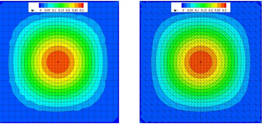
Figure 8: The final distribution of thewvelocity for a square subdomain of the manufactured solution field with sizeL/2Left: For a spatially
refined unstructured hexahedral mesh.Right: For a spatially refined unstructured prismatic mesh.
Introducing this flow field into Equations (1) we obtain analytical expressions for the source termwd. This source
term balances viscous forces and sustains the steady state manufactured solution (32). Due to the spatial and temporal discretisation errors, this solution is distorted. A small timestep and an implicit time marching scheme [16] are used to keep the temporal error low. The error of the numerical solution, compared with the exact solution (32), is described by theL2norm [79]:
L2 =
1
VΩ
N
X
m=1
Z
Em
(u−uexact)2dV
1/2
. (33)
For the flow field described by (32), Equations (1) were integrated up tottot =0.1L/con a computational domain of
is uniformly imposed up to a levelL+1and a refined resolution∆x/2 for all the elements within a circle of diameter 0.5 around the maximum velocity point of the solution (32) as shown in Figure 8. The elements outside this area were refined to a lower levelLand a nominal resolution∆x. The final solution for hexahedral and prismatic discretisations is shown in Figure 8 (Left) and (Right). The order of the polynomial basis is uniform for all the elements. This test is introduced to assess the order of accuracy for the discretisation of our implementation, in the case of a non-conforming mesh, refinement. The maximum order of accuracy isp+1 for basis functions which are polynomials of degree p. Thus, theL2norm of the error is expected to depend on the mesh resolution∆xasL2 ∼(∆x)p+1.
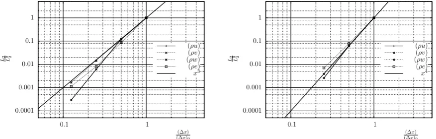
The normalised value of theL2error is presented in Figure 9 for a number of mesh sizes. Four mesh sizes were used, withN =10, 20 40 and 80 cells per direction at the edges of the domain, resulting in mesh sizes∆xequal to
∆x=L/N. For each discretisation, the core of the domain is further refined to one more level. TheL2error, defined in Equation (33), displays a second order decrease with the mesh size. Thus, the implementation of the adaptivity preserves the order of accuracy. Results similar to those shown in Figures 9, but for the third and fourth orders of accuracy, with p = 2 and p = 3 polynomial orders, are presented in Figure 10. As follows from this figure, the expected accuracy is achieved in these cases, as forp=1.
0.0001 0.001 0.01 0.1 1
0.1 1
L20 2L
(∆x) (∆x)0
(ρu) (ρv) (ρw) (ρe)
x2
0.0001 0.001 0.01 0.1 1
0.1 1
L20 2L
(∆x) (∆x)0
(ρu) (ρv) (ρw) (ρe)
[image:18.595.68.508.303.442.2]x2
Figure 9: Values of theL2error for the momentum components and energy, normalised by the value of the error for the coarse discretisation, versus
mesh resolution for the second order discretisation (p=1).Left:Hexahedral elements.Right:Prismatic elements.
0.0001 0.001 0.01 0.1 1
0.1 1
L20 2L
(∆x) (∆x)0
(ρu) (ρv) (ρw) (ρe)
x3
0.0001 0.001 0.01 0.1 1
0.1 1
L20 2L
(∆x) (∆x)0
(ρu) (ρv) (ρw) (ρe)
x4
Figure 10: Values of theL2error for the momentum components and energy, normalised by the value of the error for the coarse discretisation,
versus mesh resolution for hexahedral elements.Left:Third order discretisation (p=2).Right:Fourth order accurate discretisation (p=3).
7.2. Shock capturing
[image:18.595.68.507.479.619.2]computational efficiency of the AMR methodology. The shock angleβ, Mach number M2 and gas densityρ2 at the downstream side of the shock were calculated from the analytical expressions [71]:
tanθ=2 cotβ M 2 1sin
2β−1
M2
1(γ+cos 2β)+2
, ρ2=ρ1
(γ+1)M12sin2β
(γ−1)M12sin2β+2, M2= 1 sin(β−θ)
v t
1+γ−21M21sin2β
γM2 1sin
2β−γ−1 2
, (34)
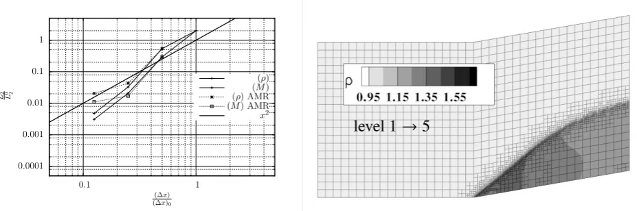
where,ρ1andM1are the density and Mach number of the gas at the upstream side, andγis the heat capacity ratio. The problem was solved numerically by integrating the inviscid form of Equations (1) on the geometry shown in Figures 11. The computational domain consists of two blocks with unity sides forming a 10◦half-wedge. The domain is discretised using 20×40 elements with base (coarse level) resolution∆x0 =0.05. For the solution presented in Figure 12 (Right) the base mesh is dynamically refined by up to five levels to a resolution of∆x=0.003125 based on the density gradient criterion. For this simulation, p1 polynomial basis was used. The shock capturing characteristics of the AMR approach resulted in the stable bounded solution without the use of the TVB limiter.
Neighbouring cells are also meshed to a gradually increasing resolution after the implementation of the smoothing pass. The three numerical solutions shown in the upper row of Figure 11 were obtained using uniform grids starting from the base resolution and reaching up to four levels of refinement (not shown). TheL2 errors of the numerical solutions for the Mach numberM2and densityρ2 are shown in Figure 12 (Right). As follows from this figure, the level of theL2error decreases as∆x2, in agreement with the prediction of the second order discretisation (p=1).
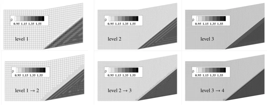
level 1 level 2 level 3
[image:19.595.35.557.343.548.2]level 1→2 level 2→3 level 3→4
Figure 11: Density distribution for the converged numerical solutions to the oblique shock problem.Top:Level 1, Level 2 and Level 3 solutions
on a uniform hexahedral mesh.Bottom:Converged AMR solutions restarted from the corresponding solutions in the upper row.
Each numerical solution shown in the top row of Figure 11 was locally refined by one more level at areas where the density gradients indicate the location of the oblique shock. The refined solutions on the uniform meshes were integrated again until their residuals converged to new values. The values of theL2 error for each refined solution are shown as the points connected with dashed lines in Figure 12 (Left). In this figure, these errors are presented as functions of the spatial resolution of the refined area.
The local refinement of a solution in the area of the shock results in the reduction of the residuals of Level n
solution to the values of Leveln+1 solution. Although the errors of the refined solutions do not reach exactly the
0.0001 0.001 0.01 0.1 1
0.1 1
L20 2L
(∆x) (∆x)0
(ρ) (M) (ρ)AMR
(M)AMR x2
[image:20.595.65.529.105.259.2]level 1
→
5
Figure 12:Left:Values ofL2errors for densityρ2and Mach numberM2, normalised with the error of the coarse discretisation at the upwind side
of the shock, versus the mesh resolution. For the AMR cases∆xcorresponds to the refined cell size.Right:Intermediate solution for densityρ2
during the formation of the oblique shock for an AMR scheme from the base level 1 up to level 5.
7.3. Computational efficiency
In this section we perform an assessment of the computational efficiency of the AMR implementation. The assessment is carried out for two problems. Firstly, the numerical solution of the three-dimensional problem of the oblique shock presented in the previous section. Computationally, this specific case represents problems where the complexity arising from the solution drives a gradual increase in the degrees of freedom of the simulation. In this test, we assess the scaling of the computational cost as the topological forest develops. The second problem is a typical viscous problem of the flow around a cylinder at Re= 500.0. In this case we assess the performance of the AMR methodology for a developed AMR forest which is periodically re-adapted to resolve the moving vortical structures.
In Figure 13 we present the solution to the oblique shock problem on a domain consisting of two prisms joint on their triangular faces so that their rectangular bases form a 10◦ half-wedge. The initial mesh consists of only two prisms. Each of these prisms is uniformly refined up to five levels. The density gradient is used to identify the elements intersected by the oblique shock. These elements are further refined up to nine levels. This demonstrates the ability of the method to capture flow structures. In this specific case, the initial ancestral mesh with sizeN=2, finally reachesN ∼30.000 elements. These elements follow the evolution of the oblique shock to the steady state solution. For technical reasons, the domain decomposition is restricted to two computational domains, since the ancestral mesh consists of only two trees. As described in Section 4.2, the forest graph is dynamically repartitioned. Although most of the new trees reside under the second ancestral tree (the prism on the ramp), they are equally distributed among the two processors.
In Figure 13 (Right) we present the CPU time per timestep, for the first 300 steps of simulation when the mesh starts from 16 elements (using oct-tree splitting, the two initial cells are split into 16 cells at the start of the simulation) and reachesN = 11.685 trees after the 300th iteration. The mesh is refined every 10 timesteps to account for the changes in the flow structure. As can be seen in Figure 13 (Right) the computational cost of AMR is 2−3 times greater than the actual cost of the integration of the governing equations for the Euler explicit time advancement scheme. For the interval of 10 timesteps, however, the computational overheads due to the use of the AMR sum up to between 20% and 30% of the total computational time. The benefits of usingAMRare even more clearly seen if we consider the computational cost needed for reaching the required resolution in three dimensional cases for uniform meshes. In this case the number of cells for a 9 times finer mesh would have been of the order of 107. This is two to three orders of magnitude greater than the number of cells needed to reach the same resolution using AMR.
In order to assess the computational cost breakdown for the different steps of the AMR methodology, we carried out an AMR simulation for the case of the viscous subsonic flow around a cylinder with diameterD. The far field velocity isU0 =0.3cand the macroscopic Reynolds number is ReD= cMDν =500.0, wherecis the speed of sound.
0.001 0.01 0.1 1 10
0 50 100 150 200 250 300
Iteration
[image:21.595.78.507.120.290.2]CPU Time (sec) Mesh size×104
Figure 13:Left:Density distribution for the oblique shock problem discretised with prismatic elements. Light (yellow) iso-surface indicates the
ρ=1.05 contour.Right:Performance of the AMR algorithm for the three dimensional oblique shock simulation using oct-trees. (Solid curve):
CPU time for each timestep. (Dashed curve): Number of elements.
Figure 14:Left:AMR simulation of the flow around a cylinder atReD=500. The contour levels range from white to red and correspond to the
vorticity magnitude. The red and blue iso-surfaces correspond to the lateral velocity levelsw=±0.05M. The positive and negative lateral velocities show the three dimensional structure at the location of the lambda vortices which connects the main trailing vortices of the wake (rollers). Only the elements with vorticity magnitude larger than 0.25 are shown, in order to reveal the structure of the oct-tree split mesh.
[image:21.595.70.527.342.606.2]Number of CPU’s (nodes×cores ) 1×20 1×40 2×40 4×40
Process Units Time breakdown
Solution (%) 84.82 74.97 64.43 53.25
Communication (%) 9.51 8.99 10.88 8.46
Gradients (%) 18.68 13.80 9.70 6.05
Adaptation (%) 13.56 21.98 31.05 38.86
Connectivity (%) 1.00 1.65 2.28 2.80
Partitioning (%) 1.62 3.05 4.52 7.88
Exchange (%) 1.21 2.14 2.56 3.68
[image:22.595.157.441.121.263.2]Time (s) 6331.0 5404.0 3449.0 2397.0
Table 1: AMR computational cost breakdown.
refined every 100 steps. A characteristic displacement of the conveyed structures for this adaptation interval is 0.03D, which corresponds to the smallest mesh size of the problem (The boundary layer elements size is 0.02D, allowing the resolution of the boundary layer structure at the wall withy+ ∼ 1). With this set-up, the vortical structures are always within the refined domain, allowing the potential for even greater adaptation intervals than the 100 steps at the far-field.
1 10 100 1000
0 500 1000 1500 2000
Num
ber
of
elemen
ts
×
1000
Time-step Elements per partition (1x20 cores) Elements per partition (4x40 cores) Total number of elements
Figure 15: Evolution of the total number of elements for the three dimensional simulation of the viscous flow around a cylinder withL/D=4.
(Solid curve): Total number of elements. (Dashed curve): Number of elements in each partition. Circles correspond to a 4×40 cores simulation
and solid circles to a 1×20 cores simulation.
[image:22.595.157.421.370.585.2]