Real-Time Setup with PD and Backstepping Control for a Pelican Quadrotor

(1)

City, University of London Institutional Repository

Citation

:

Ruiz, J. A. D. and Aouf, N. ORCID: 0000-0001-9291-4077 (2017). Real-Time

Setup with PD and Backstepping Control for a Pelican Quadrotor. In: Gusikhin, O. and

Madani, K. (Eds.), Proceedings of the 14th International Conference on Informatics in

Control, Automation and Robotics. (pp. 676-681). SciTePress. ISBN 978-989-758-263-9

This is the accepted version of the paper.

This version of the publication may differ from the final published

version.

Permanent repository link:

http://openaccess.city.ac.uk/22089/

Link to published version

:

Copyright and reuse:

City Research Online aims to make research

outputs of City, University of London available to a wider audience.

Copyright and Moral Rights remain with the author(s) and/or copyright

holders. URLs from City Research Online may be freely distributed and

linked to.

City Research Online:

http://openaccess.city.ac.uk/

publications@city.ac.uk

(2)

Real-Time Setup with PD and Backstepping Control for a Pelican

Quadrotor

Jose Alejandro Dena Ruiz

1

, Nabil Aouf

2

1,2_{Centre for Electronic Warfare, Information and Cyber, Defence Academy of the United Kingdom}

Cranfield University, Shrivenham, SN6 8LA United Kingdom

{j.a.dena-ruiz, n.aouf}@cranfield.ac.uk

Keywords: PD control, Backstepping control, Kalman Filter, Optitrack, ROS.

Abstract: In this paper, a real-time setup and an implementation of a Proportional Derivative (PD) controller for ori-entation and comparison between PD and BackStepping (BS) controllers for linear positioning are presented using a Pelican quadrotor from Ascending Technologies (AscTec). An onboard Inertial Measurement Unit (IMU) was used for orientation control and Optitrack Vision Tracking System for linear positioning control. A linear Kalman filter was implemented for linear velocity estimation. The software and hardware integration was achieved with the help of the Robot Operating System (ROS). Simulations and experiments with this drone platform are achieved in order to implement different controller algorithms and analyse them in order to achieve better aircraft performance.

1 INTRODUCTION

The studies in quadrotor control designing have been increasing rapidly in recent years. Linear controllers design for quadrotors have been achieved in sev-eral work, like the Linear Quadratic Regulator(LQR) and a Proportional Integral Derivative (PID) (Khatoon et al., 2014) (Reyes-Valeria et al., 2013). Nonlinear control design has also been achieved with different techniques, like Backstepping (Das et al., 2009), Slid-ing Mode (Runcharoon and Srichatrapimuk, 2013) and Feedback Linearisation (Saif, 2009). (Castillo et al., 2005) compared the performance of a nonlin-ear control algorithm with a LQR control law. Results show the unstable response of a linear controller ap-plied to a nonlinear system, while the nonlinear con-troller shows stable response. (Gomes et al., 2016) used an AR.Drone quadrotor and a Vicon motion cap-ture system to track a moving target with a Propor-tional Derivative (PD) controller for linear position-ing. (Mashood et al., 2016) showed experimental re-sults of two AR.Drone following a squared path us-ing VICON system and MATLAB/SIMULINK for

feedback and control implementation. This was

possible with AR Drone Simulink Development Kit (ARDSDK). (Campbell et al., 2012) showed the de-sign and implementation of a quadrotor aircraft au-topilot, allowing the UAV to take off, transit from one location to another and land at a desired

loca-tion. The position data is obtained from an Opti-track system and a PID control technique was used

to achieve the desired response for (X,Y,φ,θ) and PD

controller for (Z,ψ), the integration of the motion

system and the controllers were developed on MAT-LAB/SIMULINK.

An improved PID controller was implemented by (Zheng et al., 2016) showing the comparison against the traditional PID and Backstepping (BS). Simula-tion and experimental results show stability and track-ing performance, ustrack-ing a motion capture system and MATLAB/SIMULINK as the feedback measurement and the platform for control implementation respec-tively.

(Corona-Sanchez and Rodriguez-Cortes, 2013) presented outdoor and indoor experimental validation of a nonlinear controller for a quadrotor vehicle. Also showed a real-time programming strategy, parameter identification technique and a nonlinear gain tuning procedure.

(3)

Backsepping controllers are presented to demonstrate the efficiency of ROS and optitrack at 120 Hz. This way the setup remains open for the development and implementation of a new control techniques.

2 THE QUADROTOR DYNAMIC

MODEL

[image:3.595.98.264.302.401.2]

The model is derived based on some assumptions, in order to simplify the dynamics of the complex sys-tem to be suitable for simulation and control design, Figure 1. A symmetric and rigid structure, rigid pro-pellers and ground effect has been ignored. The full Model derivation can be found on (Bouabdallah and Siegwart, 2005).

Figure 1: Quadrotor AscTec Pelican and inertial frame on Gazebo Simulator.

Using Newton’s laws of Mechanics and Euler’s Dynamics equation, the model consists of six equa-tions for the system dynamics and four equaequa-tions de-scribing the inputs of the system:

¨

X= (cosφsinθcosψ+sinφsinψ)1

mU1 (1)

¨

Y = (cosφsinθsinψ−sinφcosψ)1

mU1 (2)

¨

Z= (cosφcosθ)1

mU1−g (3)

¨

φ=θ˙ψ(˙ Iyy−Izz

Ixx

)−Jr

Ixx

˙

θΩ+U2

Ixx

(4)

¨

θ=φ˙ψ(˙ Izz−Ixx

Iyy

) + Jr

Iyy

˙

φΩ+U3

Iyy

(5)

¨

ψ=φ˙θ(˙ Ixx−Iyy

Izz

) +U4

Izz

(6)

where equation 1, 2 and 3 describe the linear

ac-celeration of the vehicle in the direction ofOx,Oyand

Oz axes using the North, East, Down (N, E, D)

con-vention respectively, while equations 4, 5 and 6 rep-resent the angular accelerations of the vehicle about

the same axes respectively. lcorresponds to the arm

length holding the propeller,φ,θandψ, represent the

Euler angles about the body axesBx, By andBz

re-spectively.Ixx,IyyandIzz, are the inertial components

about the x-axis, y-axis and z-axis respectively. ˙x, ˙y

and ˙zare the translational velocity components along

the main axes. Ui ≡1,2,3,4 represents the system

inputs.

U1=

_∑

Ti=b(Ω21+Ω22+Ω23+Ω24) (7)

U2= (−T2+T4) =bl(−Ω2₂+Ω2₄) (8)

U3= (T1−T3) =bl(Ω21−Ω23) (9)

U4= (−1)i

∑

MDi=d(−Ω

2

1+Ω22−Ω23+Ω24)

(10)

Ω=Ω2+Ω4−Ω1−Ω3 (11) where equation 7 represents the total thrust, 8 the pitch moment, 9 the roll moment and 10 perform the

yaw moment. b is the thrust factor in hover and d

is the drag factor in hover. Increasing or decreasing of the speed of the four propellers together will be responsible for the altitude (z-axis) change in posi-tion and velocity while varying the speed of one pair

of propellers (Ω3 andΩ1) will cause the aircraft to

tilt about the y-axis which is denoted as pitch angle

θ. Similarly varying the speed of the propellers pair

(Ω4andΩ2) will cause the aircraft to tilt about x-axis

which is denoted as roll angle φ. Finally the vector

summation of the reaction moment produced by the

rotation of the pair (Ω3andΩ1) and the reaction

mo-ment produced by the rotation of the pair (Ω4andΩ2)

will cause the quadrotor to spin about its axis (z-axis),

which is denoted as yaw angleψ.

3 QUADROTOR CONTROLLERS

In this section, a PD and Backstepping controller were implemented for linear positioning, while only PD controllers for orientation.

A set of PD controllers have been chosen for the UAV attitude based on the good response in simula-tions and experiments, fast response and less than five percentage error in steady state. The Euler angles are used as feedback signals to the proposed controller in order to achieve the desired orientation. Traditional implementation can be defined as:

U=Kpe(t) +Kd

de

dt (12)

WhereKpis the proportional gain,Kdthe

[image:3.595.102.285.500.650.2]

(4)

controlled value and the desired value. In our case, three PD individual controllers are implemented:

U2=Kpφ(dφ−φ) +Kdφ(dφ˙−φ)˙ (13)

U3=Kpθ(dθ−θ) +Kdθ(dθ˙−θ)˙ (14)

U4=Kpψ(dψ−ψ) +Kdψ(dψ˙−ψ)˙ (15)

Where 13, 14 and 15 represent the torques for each

axis due to the rotor’s thrust, τφ, τθ andτψ

respec-tively. Kpφ, KpθandKpψ are the proportional gains

for each controller andKdφ,KdθandKdψthe

deriva-tive ones.dφ,dθanddψare the desiredpitch,rolland

yaw,φ,θandψcorrespond to the current attitude and

position values.

Considering that desired position dx, dy, dz are

known andx,y,zcan be measured, the equations 1, 2

and 3 can be solved in order to determine the control variables:

U1= 1

cosφcosθ(r3+mg) (16)

dφ=arcsin(

m

U1

(r1sinψ−r2cosψ)) (17)

dθ=arcsin(

m

U1

(r1cosψ+r2sinψ)) (18)

Where 16 is the force to control the vertical

dis-placementz, 17 and 18 are the desired angles to

posi-tion the drone at the desiredxandyon the cartesian

plane respectively.r1andr2represent the output

con-trol signal of the desired concon-trol technique that will

be mapped to the desired angles,gis the acceleration

due to the gravity force andmis the aircraft mass.

Equations 19-21 represent the PD controllers for the linear position of the UAV.

r1=Kpx(dx−x) +Kdx(dx˙−x˙) (19)

r2=Kpy(dy−y) +Kdy(dy˙−y˙) (20)

r3=Kpz(dz−z) +Kdz(dz˙−z˙) (21)

Using the Backstepping approach, one can synthe-sise the control law forcing the system to follow the desired trajectory. Writing the model equations for linear position in space-state:

x1=x (22)

x2=x˙1=x˙ (23)

x3=y (24)

x4=x3˙ =y˙ (25)

x5=z (26)

x6=x˙5=z˙ (27)

First, we consider the tracking-error forx1

posi-tion:

z1=x1d−x1 (28)

then, by considering the lyapunov functionz1

pos-itive definite and it’s time derivative negative semi-definite:

V(z1) =

1

2z

2

1 (29)

˙

V(z1) =z1(x˙1d−x˙2) (30)

The stabilisation ofz1can be obtained by

intro-ducing the virtual control inputx2:

x2=x1˙d+α1z1 (31)

with:α1>0 (32)

∴V˙(z1) =−α1z2₁ (33)

Now, we have to makex2=x˙1d+α1z1creating

the variablez2:

z2=x2−x˙1d−α1z1 (34)

For the second step, we consider the augmented Lyapunov function:

V(z1,z2) =

1

2(z

2

1+z22) (35)

(36)

and it’s time derivative is:

˙

V(z1z2) =z2r1−z2(X¨1d−α1(z2+α1z1))−z1z2−α1z21

(37)

Extractingr1and making ¨X1d=0 is satisfied that

˙

V(z1z2)<0, now adding the termα2z2withα2>0 to

stabilisez1and we apply the same procedure for they

andzaxis:

r1=z1−α1(z2+α1z1)−α2z2 (38)

r2=z3−α3(z4+α3z3)−α4z4 (39)

r3=z5−α5(z6+α5z5)−α6z6 (40)

with:

z3=x3d−x3 (41)

z4=x4−x˙3d−α3z3 (42)

z5=x5d−x5 (43)

(5)

4 THE PELICAN PLATFORM

[image:5.595.85.274.223.305.2]

The Pelican quadrotor from AscTec was chosen as the prototype to develop the experiments, it’s physical ar-chitecture made of carbon fibre and well distributed sensors and components make it a reliable platform for research purposes. This Quadrotor offers plenty of space and various interfaces for individual compo-nents and payloads. The total quadrotor weight in-cluding sensors and battery is 1.63 Kg. Figure 2.

Figure 2: Quadrotor AscTec Pelican with Autopilot and Mastermind.

[image:5.595.89.271.477.608.2]

The basic electronic components are the AscTec Autopilot, Motor controllers and a single board com-puter, the Mastermind. The AscTec Autopilot also known as Flight-Control-Unit (FCU) contains the High Level Processor and the Low Level Processor (HLP and LLP) running at 1 Khz which are in charge of the aircraft control. The overall architecture is pre-sented on Figure 3, the LLP handles sensor data pro-cessing, data fusion as well as an stable attitude con-trol algorithm. The HLP is open for user purposes, to implement control algorithms, sensor fusion, etc.

Figure 3: Autopilot electronic architecture.

The AscTec Mastermind is an onboard processor board, which can be carried by the AscTec Pelican, it can be used like a ground PC, but it is mounted on the flight system. In comparison to its weight and size, it offers an extremely high processing power, high data rates and a great variety of standard PC in-terfaces to connect several kind of hardware devices. Features like a Dual Core Atom, a Core 2 Duo, or a

Core i7, Firewire, WIFI and hardware serial ports are supported.

5 THE QUADROTOR CONTROL

SYSTEM

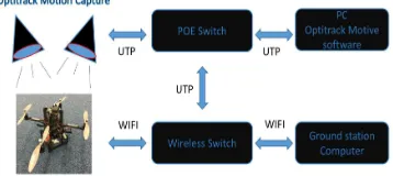
The complete Quadrotor control system is presented on figure 4. The full system is composed by the Pel-ican from AscTec, which is the platform to control. The PD orientation controllers obtained on equations 13, 14 and 15 were implemented in the HLP on Peli-can, these controllers are using the angles provided by the LLP as the feedback measurements. In the AscTec Mastermind, a ROS application is interacting with the HLP through the serial port, this application is send-ing the new desired angles and receivsend-ing the current states of the control variables and gives the user the possibility of a real-time gain tuning. Figure 4 shows the full control system overview.

Once the orientation controller is working, a sec-ond ROS application is running parallel on the As-cTec Mastermind, this application is performing the linear position control algorithms for the Drone, al-lowing the user to choose between the PD or BS con-trollers obtained in section 3, create trajectories and test new different control techniques. An Optitrack Motion Capture System was used to retrieve the ac-tual Drone position with a precision up to 2 mm. A setup of 6 cameras connected to a 12-port POE switch along with a host computer, Optitrack Motive appli-cation runs and streams the current position of a rigid body at 120 Hz to the AscTec Mastermind through a wifi router. This second application also allows the user to select between a PD or Backstepping con-troller for linear position as well as real-time gain tun-ing.

Figure 4: Quadrotor Control System overview.

6 EXPERIMENTAL RESULTS

[image:5.595.326.505.545.625.2]

(6)

an-gular velocities were obtained from the onboard

au-topilot IMU, whereas to retrieve theX,Y andZ

posi-tion the optitrack system was used. A ROS package was used to publish into ROS network the position of the rigid body and the use of a linear Kalman filter for velocity estimation. A two metres squared trajectory was chosen as the drone trajectory and altitude of one metre.

Velocity estimation was achieved using the linear Kalman filter based on (Kim, 2010). Optitrack system provides a high accuracy on ground truth at 120 Hz (dt=0.0083), taking this parameters into account and

the time-varying for the process noise matrixQ, the

values of the matrices resulted as follow:

A=       

1 0 0 dt 0 0

0 1 0 0 dt 0

0 0 1 0 0 dt

0 0 0 1 0 0

0 0 0 0 1 0

0 0 0 0 0 1

       (45) H=  

1 0 0 0 0 0

0 1 0 0 0 0

0 0 1 0 0 0



 (46)

R=





4X10−6 0 0

0 4X10−6 0

0 0 4X10−6

  (47) Q=       

0 0 0 0 0 0

0 0 0 dt2 0 0

0 0 0 0 dt2 0

0 0 0 0 0 dt2

       (48)

0 500 1000 1500 2000 2500 3000 3500 4000 4500 5000 time in (ms)

0 0.2 0.4 0.6 0.8 1 1.2

Altitude in metres

Altitude PD controller

0 500 1000 1500 2000 2500 3000 3500 4000 4500 5000 time in (ms)

-1 -0.5 0 0.5 1

Y position in metres

Y trajectory PD controller

0 500 1000 1500 2000 2500 3000 3500 4000 4500 5000 time in (ms)

-2.5 -2 -1.5 -1 -0.5 0 0.5

X position in metres

[image:6.595.323.505.97.232.2]

X trajectory PD controller

Figure 5: Real XYZ displacement with a PD controllers

Figures 5-7 show the results in real-time using the PD controllers and Figures 8-10 show the results for the BS controllers.

0 500 100015002000250030003500400045005000

time in (ms) -0.06 -0.04 -0.02 0 0.02 0.04 0.06 YAW( ) angle in radians

YAW( ) PD controller

0 500 100015002000250030003500400045005000

time in (ms) -0.015 -0.01 -0.005 0 0.005 0.01 Nm

YAW Torque control

0 500 100015002000250030003500400045005000

time in (ms) -0.4 -0.2 0 0.2 0.4 ROLL( ) angle in radians

ROLL( ) PD controller

0 500 100015002000250030003500400045005000

time in (ms) -0.06 -0.04 -0.02 0 0.02 0.04 0.06 Nm

ROLL Torque control

0 500 100015002000250030003500400045005000

time in (ms) -0.3 -0.2 -0.1 0 0.1 0.2 0.3 PITCH( ) angle in radians

PITCH( ) PD controller

0 500 100015002000250030003500400045005000

time in (ms) -0.06 -0.04 -0.02 0 0.02 0.04 0.06 Nm

PITCH Torque control

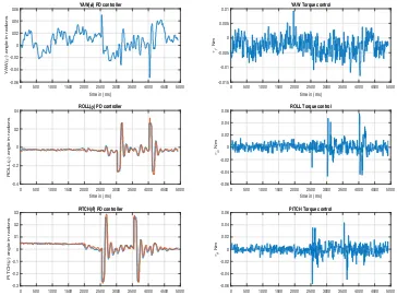
Figure 6: Real Torques and desired angles ROLL, PITCH and YAW with a PD controllers

1 0 -2.5 0.2 0.5 0.4 -2

X-Y-Z trajectory PD controller

0.6

Z position in metres

0 -1.5

0.8

Y position in metres 1

[image:6.595.89.285.266.670.2]

-1 -0.5 1.2 -0.5 -1 0 -1.5 0.5 Desired Trajectory Trajectory

Figure 7: Real 3D trajectories using a PD controllers

0 500 1000 1500 2000 2500 3000 3500 4000 time in (ms)

0 0.2 0.4 0.6 0.8 1 1.2

Altitude in metres

Altitude BS controller

0 500 1000 1500 2000 2500 3000 3500 4000 time in (ms)

-1 -0.5 0 0.5 1

Y trajectory BS controller

0 500 1000 1500 2000 2500 3000 3500 4000 time in (ms)

-2.5 -2 -1.5 -1 -0.5 0 0.5

[image:6.595.322.505.275.408.2]

X trajectory BS controller

Figure 8: Real XYZ displacement with a BS controllers

7 CONCLUSIONS

[image:6.595.321.505.436.572.2]

(7)

al-0 500 1000 1500 2000 2500 3000 3500 4000 time in (ms)

-0.02 0 0.02 0.04 0.06 0.08 0.1 YAW( ) angle in radians

YAW( ) PD controller

0 500 1000 1500 2000 2500 3000 3500 4000 time in (ms) -15 -10 -5 0 5 Nm

10-3 YAW Torque control

0 500 1000 1500 2000 2500 3000 3500 4000 time in (ms)

-0.3 -0.2 -0.1 0 0.1 0.2 0.3 ROLL( ) angle in radians

ROLL( ) PD controller

0 500 1000 1500 2000 2500 3000 3500 4000 time in (ms) -0.1 -0.05 0 0.05 0.1 Nm

ROLL Torque control

0 500 1000 1500 2000 2500 3000 3500 4000 time in (ms)

-0.3 -0.2 -0.1 0 0.1 0.2 0.3 PITCH( ) angle in radians

PITCH( ) PD controller

0 500 1000 1500 2000 2500 3000 3500 4000 time in (ms) -0.1 -0.05 0 0.05 0.1 Nm

[image:7.595.87.272.97.233.2]

PITCH Torque control

Figure 9: Real Torques and desired angles ROLL, PITCH and YAW with a BS controllers

1 0 -2.5 0.2 0.5 -2 0.4 0.6

X-Y-Z trajectory BS controller

-1.5 0

Z position in metres

0.8

-1 -0.5 1 -0.5 1.2 -1 0 -1.5 0.5 Desired Trajectory Trajectory

Figure 10: Real 3D trajectories using a BS controllers

gorithms were developed under C++ and ROS, which allow us to create a network where the ground sta-tion, robots and sensors can exchange information at 120 Hz. The Drone performance was tested using an square trajectory with 2 metres side, which was enough to move the desired roll and pitch angles and see their control response with the PD controller. The desired angles was reached within a short period of time, for instance 0.25 rad in 100 ms on the experi-mental results for roll angle as figure 6 shows. Re-garding positioning control, a linear PD controller and a non linear Backstepping controller were tested,

get-ting a better response forX andY position with the

Backstepping controller in figure 8 than the PD in

fig-ure 5, whereas for the altitudeZthe PD controller had

a quicker response compared with BS as shown in fig-ures 7 and 10.

REFERENCES

Bouabdallah, S. and Siegwart, R. (2005). Backstepping and sliding-mode techniques applied to an indoor micro quadrotor. Proceedings - IEEE International

Confer-ence on Robotics and Automation, 2005(April):2247– 2252.

Campbell, J., Hamilton, J., Iskandarani, M., and Givigi, S. (2012). A systems approach for the development of a quadrotor aircraft. InSysCon 2012 - 2012 IEEE In-ternational Systems Conference, Proceedings, pages 110–116.

Castillo, P., Lozano, R., and Dzul, A. (2005). Stabilization of a mini rotorcraft with four rotors: Experimental implementation of linear and nonlinear control laws.

IEEE Control Systems Magazine, 25(6):45–55. Corona-Sanchez, J. J. and Rodriguez-Cortes, H. (2013).

Ex-perimental real-time validation of an attitude nonlin-ear controller for the quadrotor vehicle. In2013 Inter-national Conference on Unmanned Aircraft Systems, ICUAS 2013 - Conference Proceedings, pages 453– 460.

Das, A., Lewis, F., and Subbarao, K. (2009). Backstepping approach for controlling a quadrotor using lagrange form dynamics. Journal of Intelligent and Robotic Systems: Theory and Applications, 56(1-2):127–151. Gomes, L. L., Leal, L., and Oliveira (2016). Unmanned

quadcopter control using a motion capture system.

IEEE Latin America Transactions, 14(8):3606–3613. Khatoon, S., Gupta, D., and Das, L. K. (2014). Pid &

lqr control for a quadrotor: Modeling and simulation.

Proceedings of the 2014 International Conference on Advances in Computing, Communications and Infor-matics, ICACCI 2014, pages 796–802.

Kim, P. (2010).Kalman Filter for Beginners with MATLAB Examples. A-JIN, Republic of Korea, 1 edition. Mashood, A., Mohammed, M., Abdulwahab, M.,

Abdul-wahab, S., and Noura, H. (2016). A hardware setup for formation flight of uavs using motion tracking sys-tem. InISMA 2015 - 10th International Symposium on Mechatronics and its Applications.

Reyes-Valeria, E., Enriquez-Caldera, R., Camacho-Lara, S., and Guichard, J. (2013). Lqr control for a quadrotor using unit quaternions: Modeling and simulation bt -electronics, communications and computing (coniele-comp), 2013 international conference on. pages 172– 178.

Runcharoon, K. and Srichatrapimuk, V. (2013). Slid-ing mode control of quadrotor. 2013 International Conference on Technological Advances in Electrical, Electronics and Computer Engineering (TAEECE), (1):552–557.

Saif, A. A. H. (2009). Quadrotor control using feedback linearization with dynamic extension.2009 6th Inter-national Symposium on Mechatronics and its Applica-tions, ISMA 2009, (1):25–27.

[image:7.595.87.271.271.408.2]