Identification and estimation of a large factor model with structural instability

City, University of London Institutional Repository

Citation

: Baltagi, B. H., Kao, C. and Wang, F. (2017). Identification and estimation of a

This is the accepted version of the paper.

This version of the publication may differ from the final published

version.

Permanent repository link:

Link to published version

: http://dx.doi.org/10.1016/j.jeconom.2016.10.007

Copyright and reuse:

City Research Online aims to make research

outputs of City, University of London available to a wider audience.

Copyright and Moral Rights remain with the author(s) and/or copyright

holders. URLs from City Research Online may be freely distributed and

linked to.

City Research Online: http://openaccess.city.ac.uk/ [email protected]

IDENTIFICATION AND ESTIMATION OF A LARGE FACTOR

MODEL WITH STRUCTURAL INSTABILITY

Badi H. Baltagi

Syracuse University

Chihwa Kao

Syracuse University

Fa Wang

Syracuse University

February 25, 2016

Abstract

This paper tackles the identi…cation and estimation of a high dimensional factor model with unknown number of latent factors and a single break in the number of factors and/or factor loadings occurring at unknown common date. First, we propose a least squares estimator of the change point based on the second moments of estimated pseudo factors and show that the estimation error of the proposed estimator is Op(1). We also show that the proposed estimator has some degree of robustness to misspeci…cation of the number of pseudo fac-tors. With the estimated change point plugged in, consistency of the estimated number of pre and post-break factors and convergence rate of the estimated pre and post-break factor space are then established under fairly general assump-tions. The …nite sample performance of our estimators is investigated using Monte Carlo experiments.

Keywords: high dimensional factor model, structural change, rate of con-vergence, number of factors, model selection, factor space, panel data

JEL Classi…cation: C13; C33.

1

Large factor models where a large number of time series are simultaneously driven by a small number of unobserved factors, provide a powerful framework to analyze high dimensional data. In the past …fteen years, large factor models have been success-fully used in business cycle analysis, consumer behavior analysis, asset pricing and economic monitoring and forecasting, see for example Bernanke, Boivin and Eliasz (2005), Lewbel (1991), Ross (1976) and Stock and Watson (2002b), to mention a few. Estimation theory of large factor models also experienced some breakthroughs, see Bai and Ng (2002) and Bai (2003), to mention a few. While most applications implic-itly assume that the number of factors and factor loadings are stable, there is broad evidence of structural instability in macroeconomic and …nancial time series. Stock and Watson (2002a, 2009) argue that given the number of factors, standard principal component estimation of factors is still consistent if the magnitude of the factor load-ing break is small enough. Bates, Plagborg-Møller, Stock and Watson (2013) further argue that a su¢ cient condition for consistent estimation of the factor space is that the magnitude of the factor loading break should converge to zero asymptotically. The condition becomes increasingly stringent if one is to ensure the same conver-gence rate of the estimated factor space derived in Bai and Ng (2002). This plays a crucial role in subsequent forecasting and factor augmented regression models, and in ensuring consistent estimation of the number of factors. However, in many empirical applications, the magnitude of factor loading break could be large and the number of factors may also change over time. Examples include important economic events such as the European debt crisis, or political events such as the end of the cold war, or policy change such as the end of China’s one-child policy, to mention a few.

estimated number of factors will be transmitted to the estimated factors. In such cases, it is hard to interpret the estimated factors, and forecasting performance may also deteriorate since adding extra factors in the forecasting equation does not always control the true factor space1_{. Consequently, a series of tests are proposed to test}

large factor loading break, including Breitung and Eickmeier (2011), Chen, Dolado and Gonzalo (2014), Han and Inoue (2015) and Corradi and Swanson (2014). Once a large factor loading break has been detected, one still has to estimate the change point, determine the number of pre and post-break factors and estimate the factor space.

In fact, identi…cation and estimation of a factor model in the presence of structural instability have inherent di¢ culties. First, without knowing the change point, it is infeasible to consistently estimate the factors and factor loadings even if the number of pre-break and post-break factors were known. Second, existing change point esti-mation methods require knowledge of the number of regressors and observability of the regressors, see for example Bai (1994, 1997, 2010). Hence, to estimate the change point along this path, even if the number of pre-break and post-break factors were known, we still need at least a consistent estimator of the factors, which is infeasible without knowing the change point. For example, consider the case where the number of factors is known, constant over time and after a certain time period, the factor loadings are all doubled. This model can be equivalently represented as the model where factor loadings are constant over time, while factors are all doubled after that time period. In this case, estimating the change point directly following Bai (1994, 1997) is not promising. Cheng, Liao and Schorfheide (2015) propose a shrinkage procedure that consistently estimates the number of pre and post-break factors and consistently detects factor loading breaks when the number of factors is constant, without requiring knowledge of the change point. This result is a signi…cant break-through. However, it only leads to a consistent estimate of the change fraction and does not lead to consistent estimates of the factors or factor loadings. In addition,

1_{Consider the case where all factor loadings are doubled after the change point. Also, the number}

Chen (2015) also proposes a consistent estimate of the change fraction.

In contrast with Cheng, Liao and Schorfheide (2015), we …rst propose a least squares estimator of the change point without requiring knowledge of the number of factors and observability of the factors. Based on the estimated change point, we then split the sample into two subsamples and use each subsample to estimate the number of pre and post-break factors as well as the factor space. The key observation behind our change point estimator is that the change point of the factor loadings in the original model is the same as the change point of the second moment matrix of the factors in the equivalent model. Estimating the former can therefore be converted to estimating the latter, thereby circumventing the estimation of the original model. This observation was …rst utilized by Chen et al. (2014) and Han and Inoue (2015) to test the presence of a factor loading break. Here we further exploit this observation to estimate the change point. More speci…cally, we start by estimating the number of pseudo factors and the pseudo factors themselves ignoring structural change. This leads us to identify the equivalent model. Based on the estimated pseudo factors, we then estimate the pre and post-break second moment matrix of the pseudo factors for all possible sample splits. The change point is estimated by minimizing the sum of squared residuals of this second moment matrix estimation among all possible sample splits.

Under fairly general assumptions, we show that the distance between the estimated and the true change point is Op(1). Although our change point estimation itself is

seen as a procedure selecting the model with the strongest identi…cation strength of the unknown change point. From this perspective, our method shares some similarity with selecting the most relevant instrumental variables (IVs) among a large number of IVs.

main extra assumption we impose is that the Hajek-Renyi inequality is applicable to the second moment process of the factors. As discussed in the next section, this assumption is more general than explicitly assuming a speci…c factor process and can be easily satis…ed. It is also worth noting that for a regularly behaved error term, our results do not rely on the relative speed of the number of subjects (N) and the time series length (T).

The rest of the paper is organized as follows. Section 2 introduces the model setup, notation and preliminaries. Section 3 discusses the equivalent representation and assumptions. Section 4 considers estimation of the change point. Section 5 considers estimation of the number of pre and post-break factors. Section 6 considers estimation of the factor space. Section 7 discusses further issues relating to the limiting distribution of the change point estimator. Section 8 reports the simulation results, while Section 9 concludes. All the proofs are given in the Appendix.

2

Consider the following large factor model with structural change in the factor loadings:

xit =

(

f0

0;t 0;i+f10;t 1;i+ei;t; if 1 t [ 0T]

f0

0;t 0;i+f10;t 2;i+ei;t; if [ 0T] + 1 t T

fori= 1; :::; N and t= 1; :::; T,

(1) where ft = (f00;t; f10;t)0. f1;t and f0;t are q and r q dimensional vectors of factors

with and without structural change in their factor loadings, respectively. 0;i is the

factor loadings of subject i corresponding to f0;t: 1;i and 2;i are factor loadings of

subject icorresponding tof1;t before and after the structural change, respectively. It

is easy to see that r q = 0 and r q > 0 correspond to the pure change case and the partial change case respectively. ei;t is the error term allowed to have temporal

and cross-sectional dependence as well as heteroskedasticity. 0 2(0;1)is the change

In matrix form, the model can be represented as:

X =

"

F0

1 00+F11 01

F0

2 00+F21 02

#

+E, (2)

where F0

1 = [f0;1; :::; f0;[ 0T]]0, F

0

2 = [f0;[ 0T]+1; :::; f0;T]0, F

1

1 = [f1;1; :::; f1;[ 0T]]0 and F1

2 = [f1;[ 0T]+1; :::; f1;T]0 are of dimensions [ 0T] (r q), [(1 0)T] (r q),

[ 0T] q and [(1 0)T] q, respectively. 0 = [ 0;1; :::; 0;N]0, 1 = [ 1;1; :::; 1;N]0

and 2 = [ 2;1; :::; 2;N]0 are of dimensions N (r q),N qand N q, respectively,

E = [e1; :::; eT]0 is of dimension T N. The matrices F10, F20, F11, F21, 0, 1, 2

and E are all unknown. In addition, 01 = [ 0; 1] = ( 01;1; :::; 01;N)0 and 02 =

[ 0; 2] = ( 02;1; :::; 02;N)0 are of dimension N r. Note that in general not only

the factor loadings but also the number of factors may have structural change. In our representation, structural change in the number of factors is incorporated as a special case of structural change in factor loadings by allowing either 01 or 02 to

be degenerate. In case the number of pre-break and post-break factors are r1 and r2

respectively, with r = max_fr1; r2g, ft and i are always r dimensional vectors and

both 01 and 02 are of dimensions N r. If r1 < r2, some columns in 01 are zeros

and the number of such columns is r2 r1. In this case, 01 is degenerate and 02

is of full rank. Similarly, if r1 > r2, some columns in 02 are zeros and 01 is of

full rank. If r1 = r2, both 01 and 02 are of full rank r. In addition, we want to

point out that although cases with either disappearing factors or emerging factors are allowed for, cases with both disappearing factors and emerging factors are not necessarily identi…able within this mathematical setup. A model withs1 disappearing

factors ands2emerging factors can be equivalently represented as a model withs1 s2

disappearing factors.

Throughout the paper, _kA_k = (trAA0₎12 denotes the Frobenius norm, !p denotes

convergence in probability,_!d denotes convergence in distribution,vec(A)denotes the vectorization of matrixA,r(A)denotes the rank of matrixA, N T = minf

p

N ;pT_g,

3

Since at least one of 01 and 02 is of full rank, for the moment, suppose that 01

is of full rank. Due to symmetry, all results can be established similarly in case

02 is of full rank. When 01 is of full rank, the rank of the N (r+q) matrix

h

0 1 2

i

is between r and r+q. Suppose h 0 1 2

i

is of rank r+q1,

where 0 q1 q, then 2 can be decomposed into 2 =

h

21 22

i

, where 21 is

of dimension N q1 and contains the columns in 2 that are linearly independent

of 01. 22 is of dimension N q2 and contains the columns in 2 that are linear

combinations of columns in h 0 1 21

i

such that 22 =

h

0 1 21

i

Z for some (r+q1) q2 matrix Z. Therefore,

h

0 1 21

i

is of full rank (r+q1) and

h

0 1

i

= h _{0 1 21} iA;

h

0 2

i

= h _{0 1 21} iB;

where A =

"

Ir 0q1 r

#

and B =

2 6 4

Ir q 0(r q) q1

0q (r q) 0q q1

0q1 (r q) Iq1

Z

3 7

5. It follows that model

(2) has the following equivalent representation with stable factor loadings:

X =

2 4

h

F0 1 F11

i h

0 1

i0

h

F0 2 F21

i h

0 2

i0

3 5+E

=

2 4

h

F₁0 F₁1

i

(h _{0 1 21} iA)0

h

F0 2 F21

i

(h _{0 1 21} iB)0

3 5+E

=

2 4

h

F0 1 F11

i

A0

h

F0 2 F21

i

B0

3

Next, de…neG= (g1; :::; gT)0 =

2 4

h

F0 1 F11

i

A0

h

F0 2 F21

i

B0

3

5 and =h _{0 1 21} i, then

X = G 0+E; (4)

gt =

(

Aft; if 1 t [ 0T]

Bft; if [ 0T] + 1 t T

, (5)

and we call r+q1 the number of pseudo factors. Equivalent representation of model

(2) was …rst formulated by Han and Inoue (2015). Here our representation is uni…ed, generalizes and complements their result. Our representation is fairly general. The big break case discussed in Chen et al. (2014) corresponds to the case q1 =q, while

the type 1, type 2 and type 3 breaks discussed in Han and Inoue (2015) correspond to the cases q1 = q, q1 = 0 and 0 < q1 < q respectively. The type 1 and type 2

changes discussed in Cheng et al. (2015) are also special cases of this representation. To ensure this equivalent representation is unique up to a rotation, it remains to show

G is asymptotically full rank, i.e., _T1 PT_t=1gtg0t p

! G for some positive de…nite G.

De…ne F =E(ftft0), G;1 =E(gtgt0) for t k0 and G;2 =E(gtgt0) for t > k0, then

G;1 = A FA0; G;2 =B FB0, (6) G = 0A FA0+ (1 0)B FB0. (7)

Proposition 1 If 0 2(0;1) and F is positive de…nite, G is positive de…nite.

For the case where 02 is of full rank, 1 can be decomposed as

h

11 12

i

, where h 0 2 11

i

is of full rank and 12 =

h

0 2 11

i

Z for some Z. De…ne =h _{0 2 11} i.

Our assumptions are as follows:

Assumption 1 (1) _Ekftk4 < M < 1, E(ftft0) = F, F is positive de…nite,

1

k0

Pk0

t=1ftft0 p

! F, _T 1_k

0

PT

t=k0+1ftf

0

t p

! F, (2) there exists d > 0 such that

kA FA0 B FB0k> d for all N.

Assumption 2 _k l;ik < 1 for l = 0;1;2, _N1 0 !0 for some positive

de…nite matrix or 1

Assumption 3 There exists a positive constantM < ₁ such that:

1 _E(eit) = 0, Ejeitj8 M, for alli= 1; :::; N; and t = 1; :::; T;

2 _E(eitejs) = ij;ts for i; j = 1; :::; N; and t; s= 1; :::; T; also

1 N T XN i=1 XN j=1 XT t=1 XT

s=1j ij;tsj M;

3 For every (t; s= 1; :::; T), _{E p}1

N

PN

i=1[eiseit E(eiseit)] 4

M.

Assumption 4 There exists a positive constantM < ₁ such that:

E(1

N XN i=1 1 p k0

Xk0

t=1fteit 2

) M;

E(1

N

XN i=1

1

p

T k0

XT t=k0+1

fteit

2

) M:

Assumption 5 There exists an M < ₁ such that:

1 _E(e0set

N ) = N(s; t) and

PT

s=1j N(s; t)j M for every t T,

2 _E(eitejt) = ij;t with j ij;tj ij for some ij and for all t = 1; :::; T, and

PN

j=1j jij M for every i N.

Assumption 6 The largest eigenvalue of _{N T}1 EE0 _{is O}

p( 21

N T

).

Assumption 7 The eigenvalues of G or G are distinct.

Assumption 8 De…ne t=vec(ftft0 F):The data generating process of factors is

such that the Hajek-Renyi inequality2 applies to the process _f t; t= 1; :::; k0g, f t; t=

k0; :::;1g, f t; t =k0+ 1; :::; Tg and f t; t=T; :::; k0+ 1g.

Assumption 9 log_NT _!0.

Assumption 10 There exists M < ₁ such that:

1 For every s= 1; :::; T, _E(sup k<k0

1

k0 k

Pk0

t=k+1 1

p

N

PN

i=1[eiseit E(eiseit)] 2

) M;

E(sup k k0

1 k Pk t=1 1 p N PN

i=1[eiseit E(eiseit)] 2

) M;

E(sup k>k0

1

k k0

Pk t=k0+1

1

p

N

PN

i=1[eiseit E(eiseit)]

2

) M;

E(sup k k0

1

T k

PT t=k+1

1

p

N

PN

i=1[eiseit E(eiseit)] 2

) M;

2 _E(sup k<k0

1

k0 k

Pk0

t=k+1 1

p

N

PN i=1 ieit

2

) M;

E(sup k k0

1 k Pk t=1 1 p N PN i=1 ieit

2

) M;

E(sup k>k0

1

k k0

Pk t=k0+1

1

p

N

PN i=1 ieit

2

) M;

E(sup k k0

1

T k

PT t=k+1

1

p

N

PN i=1 ieit

2

) M:

Assumptions 1-7 are either from or slight modi…cation of Assumptions A-G in Bai (2003). Assumption 1(1) corresponds to Assumption A in Bai (2003) and should be satis…ed within each regime. ft can be dynamic and contain their lags. Assumption

1(2) enables the identi…cation of the change point and is general enough to cover all patterns of factor loading break likely in practice. It does not matter whether B

depends on N or not, as long as the distance between the pre and post-break second moment matrix ofgt is bounded away from zero asN ! 1. If r(

h

0 1 2

i

)>

r(h _{0 1} i), then A FA0 6= B FB0. If r(

h

0 1 2

i

) = r(h _{0 1} i), then

A FA0 = F and B FB0 6= F except for some very unlikely case, for example,

some post-break factor loadings are 1 times their pre-break factor loadings. Note that here to simplify analysis, the second moment matrix of the factors is assumed to be stationary over time, since in general how to disentangle structural change in

F from structural change in factor loadings is still unclear. Assumption 2

corre-sponds to Assumption B in Bai (2003) and implies that _N1 0

01 01 01 !0 and

1

N 002 02 02 ! 0. Note that one of 01 and 02 is allowed to be degenerate.

This allows for cases with disappearing or emerging factors. In addition, 0 could

contain a small change. Let 0;i be the change of 0;i. As discussed in Bates et al.

(2013), if 0;i = p_{N T}1 i and k ik < 1 for all i, consistency of the estimated

number of factors and the factors themselves will not be a¤ected. For simplicity, we assume that 0 is stable. Assumptions 3 and 5 correspond to Assumptions C and E

should be satis…ed within each regime. This is implied by Assumptions 1 and 3 if the factors and the errors are independent. Assumption 6 is the key condition for identifying the number of factors and is implicitly assumed in Bai and Ng (2002) and required in almost all existing methods of determining the number of factors or the number of dynamic factors. For example, Onatski (2010) and Ahn and Horenstein (2013) assumeE =A"B, where" is an i.i.d. T N matrix andAandB characterize the temporal and crosssectional dependence and heteroskedasticity. This is a su¢ -cient but not necessary condition for Assumption 6. In this paper, Assumption 6 can be relaxed to "The largest eigenvalue of 1

N TEE0 is op(1)", yet still allows consistent

estimation of the number of factors. Assumption 7 corresponds to Assumption G in Bai (2003).

Assumption 8 strengthens Assumption 1(1) and imposes further requirement on the factor process. Instead of assuming a speci…c data generating process, here we only require that the Hajek-Renyi inequality is applicable to the second moment process of the factors, which incorporates i.i.d., martingale di¤erence, martingale, mixingale and so on as special cases and renders Assumption 8 in its most general form. As-sumption 10 imposes further constraints on the idiosyncratic error. AsAs-sumption 3(3) and Assumption F3 in Bai (2003) imply that the summands in Assumption 10 are uniformly Op(1). Assumption 10 strengthens this condition such that the supremum

of the average process of these summands isOp(1). Also note that stationarity is not

assumed in Assumption 10. In rare cases, Assumption 10 is not satis…ed, but we can still proceed with Assumption 9. Compared to p_NT _! 0, which is assumed in Chen et al. (2014), Han and Inoue (2015), Assumption 9 is signi…cantly weaker and much easier to be satis…ed since even when T is much larger than N, log_NT could still be very close to zero.

4

4.1

change. De…ne r~as the estimated number of factors using the information criteria in Bai and Ng (2002), we will have lim

(N;T)!1P(~r = r+q1) = 1, since model (2) can be

equivalently represented as model (3). Note that q1 could be zero, since structural

change does not necessarily lead to overestimating the number of factors. Using r~, we then estimate the factors using the principal component method. This identi…es the factors gt. As noted in (6), the second moment matrix3 of gt has a break at

the point k0: Hence, estimating change point of factor loadings can be converted

to estimating change point of the second moment matrix of gt. Although gt is not

directly observable, the principal component estimator g~t is asymptotically close to

J0_g

t for some rotation matrix J. And J p

! J0 =

1

2 _V 1_{2 as (N; T)}

! 1, where

V and are the eigenvalue matrix and eigenvector matrix of

1 2

G

1

2 _{respectively.}

Hence change point estimation using g~t will be asymptotically equivalent to using

J0gt. It is easy to see that the second moment matrix ofJ0gt shares the same change

point as that of gt. Therefore, we proceed to estimate the pre-break and post-break

second moment matrix ofgt using the estimated factorsg~t.

More speci…cally, following Bai (1994, 1997, 2010), for anyk >0we split the sam-ple into two subsamsam-ples and estimate the pre-break and post-break second moment matrix of gt as

~_{1 =} 1

k

Xk t=1g~tg~

0

t; ~_{2 =} 1

T k

XT

t=k+1~gtg~

0

t, (8)

and de…ne the sum of squared residuals as

~

S(k) = Xk

t=1[vec(~gt~g

0

t ~1)]0[vec(~gt~gt0 ~1)]+

XT

t=k+1[vec(~gt~g

0

t ~2)]0[vec(~gt~g0t ~2)].

(9)

3_{The …rst moment ofg}

t may also help identify the change point, but it requires the true factors

The least squares estimator of the change point4 _is

~

k = arg min ~S(k). (10)

Here we use S~(k) to emphasize that the sum of squared residuals is based on the estimated factors.

Remark 1 The change point estimator also can be based on g^t instead of ~gt, where

(^g1; :::;^gT)0 = ^G= ~GVN T = (~g1; :::;~gT)0VN T andVN T is diagonal and contains the …rst

r+q1 largest eigenvalues of _{N T}1 XX0 in decreasing order.

4.2

ESTI-MATOR

In what follows, we shall establish the rate of convergence of the proposed estimator, which allows us to identify the number of pre-break and post-break factors as well as the factor space. Since lim

(N;T)!1P(~r =r+q1) = 1, estimation of the change point

based onr~and the true number of pseudo factorsr+q1 is asymptotically equivalent.

The proof is similar to footnote 5 in Bai (2003). Therefore, we can treat the number of pseudo factorsr+q1 as known in studying the asymptotic properties of our change

point estimator.

De…ne~ = ~k=T as the estimated change fraction, we …rst show that~is consistent.

Proposition 2 Under Assumptions 1-8 and 9 or 10, ~ 0 =op(1).

This proposition is important for theoretical purposes. In fact, it serves as a …rst step in proving Theorem 1. Proposition 2 implies that for any > 0 and > 0,

P(~ ₂ D) > 1 for su¢ ciently large N and T, where D = _fk : _jk k0j=T g.

Using similar strategy as proving Proposition 2, we can further show that for any

>0and >0, there exist anM >0 such thatP(~k ₂DM)< for su¢ ciently large

N and T, whereDM =fk :k 2D;jk k0j> Mg. Taken together, we have:

4_{Alternatively, one referee points out that one may consider quasi-maximum likelihood estimation}

Theorem 1 Under Assumptions 1-8 and 9 or 10, ~k k0 =Op(1).

This theorem implies that the di¤erence between the estimated change point and the true change point is stochastically bounded. This is quite strong since the possible change point is narrowed to a bounded interval no matter how largeT is. Although

~

k is still inconsistent, an important observation is that ~k k0 = Op(1) is already

su¢ cient for consistent estimation of the number of pre-break and post-break factors and consistent estimation of the pre-break and post-break factor space, which will be discussed further in the next three sections.

Theorem 1 di¤ers from existing results in the change point estimation literature. First, in the current setup N goes to in…nity jointly with T, thus we should be able to achieve consistency of ~k as shown in Bai (2010) for the panel mean shift case, because largeN will help identify the change point when the change point is common across individuals. Our result is di¤erent from Bai (2010) and instead similar to the univariate case, e.g., Bai (1994, 1997), because k~ is based on g~t~gt0 which is a

…xed dimensional multivariate time series with mean shift. Second, our result is also di¤erent from Bai (1994, 1997) because in the current setup we are using estimated data ~gtg~0t rather than the raw data J0gtgt0J00 to estimate the change point, i.e., the

data g~t~gt0 contains measurement error ~gtg~0t J0gtgt0J00. Eliminating the e¤ect of this

measurement error on estimation of change point relies on largeN.

Remark 2 Proposition 2 and Theorem 1 hold with either Assumption 9 or 10, but

we do not need both. Usually Assumption 10 is satis…ed. In this case, there is no

restriction on the relative speed ofN andT going to in…nity. Even when Assumption

10 is violated, our results only require log_NT _!0, which can be easily satis…ed.

Remark 3 Note that Theorem 1 requires the covariance matrix of the factors to be

stationary, and thus is not robust to heteroskedasticity of the factors. This problem

is common in the literature, for example, it also appears in Chen et al. (2014), Han

and Inoue (2015) and Cheng et al. (2015). It is important to note that Chen (2015)’s

4.3

FACTORS ON ESTIMATION OF THE CHANGE POINT

Since our method for estimating the change point is a two step procedure, a natural question is how will the model selection error in the …rst step a¤ect the performance of the second step estimation. Although consistent model selection guarantees that asymptotically we can behave as if the true model is known a priori, the …nite sample distribution of the post model selection estimator could be dramatically di¤erent from its asymptotic limit even when the sample size is very large. This is because the probability of misspecifying the model in the …rst step may be nonignorable even when the sample size is very large if consistency of the …rst step model selection is not uniform with respect to the parameter space. The distribution of the post model selection estimator is a weighted average of its distribution given the true model is selected and given some misspeci…ed model is selected, where the weight is given by the probability of selecting that model. When the probability of misspecifying the model is indeed nonignorable and the distributions with the true model selected and with the misspeci…ed model selected are very di¤erent, we can imagine that the composite distribution could be far away from its asymptotic limit.

In the current context, the Leeb and Potscher (2005)’s criticism still applies. But, we argue that our change point estimator still has some degree of robustness to the …rst step estimation error, especially if we only care about the stochastic order of the change point estimation error. This is because if the number of pseudo factors were underestimated, ~k would be based on a subset of the second moment matrix of J0gt:

Hence there is still information to identify the change point. While if the number of pseudo factors were overestimated, no information would be lost but extra noise would be brought in by the extra estimated factors. Therefore, estimating the number of pseudo factors can be seen as a procedure selecting the model with the strongest identi…cation strength of the unknown change point. From this perspective, our method shares some similarity with selecting the most relevant instrumental variables (IVs) among a large number of IVs.

Corollary 1 For any positive integer m < r+q1 and change point estimation based

on r~= m, with J0 replaced by J0m which is of dimension (r+q1) m and contains

the …rst m columns of J0, and kJ0m0 G;1J0m J0m0 G;2J0mk > d for some d > 0 and

all N, Proposition 2 and Theorem 1 still hold.

In case r~ is …xed at some positive integer m > r +q1, we can not prove the

robustness of Proposition 2 and Theorem 1. Nonetheless, if the change point estimator were based on ^gt instead of ~gt, we can prove:

Corollary 2 For any positive integer m > r+q1 and change point estimatork^ based

on g^t and r~=m, if

p

T

N !0, Proposition 2 and Theorem 1 still hold.

Note that Corollary 1 also applies to k^. Corollary 2 shows that ^k is robust to overestimation of the number of pseudo factors. This result is similar to Moon and Weidner (2015) who show that for panel data with interactive e¤ects, the limiting distribution of the LS estimator is independent of the number of factors used in the estimation, as long as this number is not underestimated.

Remark 4 If the condition "_kJm0

0 G;1J0m J0m0 G;2J0mk> d for somed >0 and all

N" is not satis…ed for all m, estimation errors of the number of the pseudo factors

may a¤ect the uniform validity of the estimation procedure. In such case, simply

…xing ~r at the maximum number of pseudo factors may be preferred, especially when

this maximum number is small or some prior information is available.

Remark 5 As can be seen in the equivalent representation, the pseudo factors

in-duced by structural change are relatively weaker than factors with stable loadings in

the original model because a portion of their elements are zeros and the magnitude of

those nonzero elements is small if the magnitude of structural change is small. Since

underestimation is more harmful5 _{compared to overestimation, we recommend}

choos-ing a less conservative criterion in estimatchoos-ing the number of pseudo factors. We will

discuss this further in the simulation section.

5_{As discussed above, underestimation will result in loss of useful moment conditions while}

Up to now, we have only touched upon the stochastic order of ~k k0. We will

postpone the discussion of the imiting distribution and instead put more emphasis on the estimation of the pre and post-break number of factors and factor space. We will show that ~k k0 = Op(1) is a su¢ cient condition for the results in subsequent

estimation. Thus for the purpose of subsequent estimation, the limiting distribution is not needed.

5

In this section, we study how to consistently estimate the number of factors in the presence of structural instability in the factor loadings or the number of factors them-selves. We …rst relax the su¢ cient condition proposed by Bates et al. (2013) for the consistent estimation of the number of factors in the presence of structural change using the Bai and Ng (2002) information criteria. The condition they propose is

1

N k k

2

= O( 21

N T

), where is the matrix of factor loading breaks. In the current setup, = 2 1. We show, in the following proposition, that their condition can

be relaxed to 1

N k k

2

=O( 1

c N T

) for some c >0.

Proposition 3 In the presence of a single common break in factor loadings, the

estimator of the number of factors using the Bai and Ng (2002) information criteria is

still consistent if _N1 _{k k}2 =O( c1

N T) for some c >0, g(N; T)!0 and

c

N Tg(N; T)!

1, where g(N; T) is the penalty function.

The formal proof is in the Appendix. This proposition complements Theorem 2 below. Note thatccan be arbitrarily close to zero, hence our condition is much weaker than that of Bates et al. (2013). The intuition behind our result is that change in factor loadings can be treated as an extra error term and as long asc >0; the …rst r

largest eigenvalues of XX0 _{are still separated from the rest. By adjusting the speed}

speed at which _N1 _{k k}2 goes to zero, so that g1(N;T)

Nk k

2 ! 1. This may be problematic

in real applications, since whencis close to zero, not all factors are necessarily strong enough to outweigh the extra noise brought by the factor loadings breaks. And even if factors are strong enough, we still need to pin down c, which is di¢ cult. In addition, the above result is not applicable for the case where _N1 _{k k}2 = O(1), nor the case where the number of factors also change. In view of these caveats, Proposition 3 is more of theoretical importance and demonstrates how far we can go following Bates et al. (2013).

To estimate the number of pre and post-break factors in the presence of large break, we propose the following procedure: split the sample into two subsamples based on the estimated change pointk~, and then use each subsample to estimate the number of pre and post-break factors. Let r~1 and r~2 be the estimated number of

pre-break and post-break factors using the method in Bai and Ng (2002). We have the following result:

Theorem 2 Under Assumptions 1-8 and 9 or 10, lim

(N;T)!1P(~r1 = r1) = 1 and

lim

(N;T)!1P(~r2 = r2) = 1, where r1 and r2 are numbers of pre-break and post-break

factors, respectively.

Theorem 2 together with Theorem 1 identi…es model (2) and provides the basis for subsequent estimation and inference. Note that k~ k0 = Op(1) is su¢ cient

for the consistency of r~1 and r~2, i.e., consistency of the second step estimators r~1

and ~r2 does not require consistency of the …rst step estimator ~k.6 This is because

~

k k0 = Op(1) is the exact condition that guarantees the extra noise brought by

a change in factor loadings does not a¤ect the speed of eigenvalue separation. In general, the e¤ect of the error in the …rst step, which could be either estimation or model selection, on the second step estimator depends on the magnitude of the …rst step error and how the second step estimator is a¤ected by the …rst step error. In the traditional plug-in procedure, usually the …rst step error need to vanish su¢ ciently fast to eliminate its e¤ect. In the current context, although the …rst step error does

6_{When estimating the pre and post-break number of factors and factor space, we consider~k as}

not vanish asymptotically, the second step becomes increasingly less sensitive to the …rst step error as T _{! 1}. This can be seen more easily by considering the case in which T is very large while ~k k0 is bounded. Since the pre and post-break

number of factors and factor space are estimated using each subsample whose size is

O(T), misspecifying the change point by a bounded value would a¤ect their behavior very little. In other words, while large T does not help identify the change point, it increases the magnitude of misspeci…cation of change point that can be tolerated.

To better demonstrate the di¤erence between our result and traditional plug-in procedure, we sketch the key steps in proving the consistency ofr~1. The estimator of

the number of pre-break factors ~r1 is based on the pre-break subsample t = 1; :::;k~.

What we need to show is: for any >0, P(~r1 =6 r1) < for large (N; T). Based on

~

k k0 =Op(1), we have for any >0, there exists M >0 such that P( ~k k0 >

M)< for all (N; T). Based on thisM, P(~r1 6=r1) can be decomposed as

P(~r1 6=r1; k~ k0 > M)+P(~r1 6=r1; k0 M ~k k0)+P(~r1 6=r1; k0+1 ~k k0+M).

The …rst term is less than P( ~k k0 > M), hence less than for all (N; T). The

second term can be further decomposed as

Xk0

k=k0 M

P(~r1(k)6=r1;~k=k),

whereP(~r1(k)6=r1;~k =k)denotes the joint probability of ~k=k and r~1(k)6=r1 and

~

r1(k)denotes the estimated number of pre-break factors using subsamplet = 1; :::; k.

Obviously, P(~r1(k) 6=r1;k~ =k) P(~r1(k)6=r1), hence the second term is less than

Pk0

k=k0 M P(~r1(k)6=r1). Furthermore, the factor loadings in the pre-break subsample

are stable when k < k0 and for k 2 [k0 M; k0], k ! 1 at the same speed as k0,

hence we have for eachk ₂[k0 M; k0], P(~r1(k)6=r1) _M+1 for large (N; T). The

second term is therefore less than Pk0

k=k0 M M+1 = for large (N; T). The argument

for the second term also applies to the third term, except for some modi…cations. First, the third term can be decomposed similarly as

Xk0+M

k=k0+1

P(~r1(k)=6 r1;k~=k)

Xk0+M

k=k0+1

hence it remains to show for each k ₂ [k0+ 1; k0 +M], P(~r1(k)6=r1) _M for large

(N; T). Unlike the second term, whenk ₂[k0+1; k0+M]the factor loadings of the

pre-break subsamplet= 1; :::; khas a break att=k0, hence results already established for

the stable model are not directly applicable. Nevertheless, the number of observations with factor loading break,k k0, is bounded by M. Hence in estimating the number

of factors, these observations will be dominated by the observations t = 1; :::k0, as

k0 = [ 0T]! 1.

6

In this section, we discuss the estimation of the pre-break and post-break factor space. As in last section, we split the sample into two subsamples based on the change point estimatork~, and then use each subsample to estimate the pre-break and post-break factor space. For each possible sample split k, de…neX(k) = (x1; :::; xk)0,

F1(k) = (f1; :::; fk)0 and F2(k) = (fk+1; :::; fT)0. Let u be any prespeci…ed

num-ber of pre-break factors, which does not necessarily equal r1. The principal

compo-nent estimator of the pre-break factors and factor loadings are obtained by solving

V(u) = min 1

N k

Pk t=1

PN

i=1(xit ft0 i)2. Since the true factors can be identi…ed only

up to a rotation, the normalization condition has to be imposed to uniquely determine the solution, and based on di¤erent normalization conditions there are two solutions. For the …rst one, the estimated factors,F~u

1(k), equal

p

T times the eigenvectors corre-sponding to the …rstulargest eigenvalues of _{N k}1 X(k)X0_(k)and ~u

1(k) = 1

kX0(k) ~F u

1(k)

are the corresponding estimated factor loadings. For the second one, the estimated factor loadings, u1(k), equal

p

N times the eigenvectors corresponding to the …rst u

largest eigenvalues of _{N k}1 X0(k)X(k) and F₁u(k) = _N1X(k) u₁(k) are the correspond-ing estimated factors. Followcorrespond-ing Bai and Ng (2002), we de…ne the rescaled estima-tor F^u

1(k) = F1u(k)[k1F u0

1 (k)F1u(k)]

1

2. The estimator of the post-break factors F^v

2(k)

can be obtained similarly based on the post-break subsample, where v is the pre-speci…ed number of post-break factors. Next, de…ne Hu

1(k) =

0

01 01

N F0

1(k) ~F1u(k)

k and

Hv

2(k) =

0

02 02

N F0

2(k) ~F2v(k)

T k . Let f^ u

t(~k) and f^tv(~k) be the estimated factors based on

theorem:

Theorem 3 Under Assumptions 1-8 and 9 or 10,

1 ~

k

X_k~

t=1

^

f_tu(~k) H₁u0(~k)ft

2

= Op( 1

2

N T );

1

T ~k

XT t=~k+1

^

f_tv(~k) H₂v0(~k)ft

2

= Op( 1

2

N T ):

Theorem 3 implies that our estimator of the factor space is mean squared con-sistent within each regime and the convergence rate is the same as that obtained by Bai and Ng (2002) for the stable model. Consistent estimation of the factor space has proved to be crucial in many cases, including forecasting and factor augmented regressions. Note that the convergence rateOp( 21

N T

)plays a crucial role in eliminating the e¤ect of using estimated factors, for which consistency is not enough. Bates et al. (2013) show that if we ignore the structural change, consistency of the estimated factor space requires 1

N k k

2

= o(1). In contrast, to guarantee the convergence rate

Op( 21

N T

) of the estimated factor space, it requires 1

N k k

2

= O( 1

N T). While

reason-able for a small break, these two conditions especially the latter are not suitreason-able for a large break. As discussed in Banerjee, Marcellino and Masten (2008), this is the most likely reason behind the worsening factor-based forecasts. In contrast, our result allows for a large break, and hence improves and complements Bates et al. (2013).

Remark 6 Note that ~k k0 = Op(1) is both a necessary and su¢ cient condition

for Theorem 3. If ~k k0 is of order larger than Op(1), the convergence speed in

Theorem 3 will be a¤ected.

Remark 7 Theorem 3 is based on arbitrarily u and v rather than r~1 and r~2, the

estimated number of pre-break and post-break factors. On the other hand,r~1andr~2are

based directly on eigenvalue separation, without using consistency of the estimated

pre-break and post-pre-break factor space. Hence, Theorem 3 and Theorem 2 are independent

of each other. Alternatively, we can choose u = ~r1 and v = ~r2. Since r~1 and ~r2 are

consistent, this is asymptotically equivalent to the case in which r1 and r2 are known.

estimated factors. Whenr1 andr2 are known and under Assumptions 1-8 and 9 or 10,

we have _k1_~P~k_t=1 f^t(~k) H10(~k)ft

2

=Op( 21

N T

)and _T1_~kPT_t=~k+1 f^t(~k) H20(~k)ft

2

=

Op( 21

N T

).

7

To make inference about the change point, we seek to derive its limiting distribution. De…ne

yt = vec(J00gtg0tJ0 1)for t k0,

yt = vec(J00gtg0tJ0 2)for t > k0, (11)

where 1 =J00 G;1J0 and 2 =J00 G;2J0 are the pre-break and post-break means of

J0

0gtgt0J0. The limiting distribution of ~k is as follows:

Theorem 4 Under Assumptions 1-8 and 9 or 10, ~k k0

d

!arg minW(l), where

W(l) = l_k 2 1k2 2

Xk0 1

t=k0+l

[vec( 2 1)]0yt for l = 1; 2; :::,

W(l) = 0 for l = 0,

W(l) = l_k 2 1k2 2

Xk0+l

t=k0+1

[vec( 2 1)]0yt for l = 1;2; :::. (12)

Ifyt is independent overt, thenW(l)is a two-sided random walk. Note that yt is

not assumed to be stationary. By de…nition, if ft is stationary, then gt and hence yt

is stationary within each regime. In this case Pk0 1

t=k0+l and

Pk0+l

t=k0+1 can be replaced

by P_t=1_l and Pl_t=1. The main problem is that this limiting distribution is not free of the underlying DGP, hence constructing a con…dence interval is not feasible. In previous change point estimation studies, the shrinking break assumption is required to make the limiting distribution independent of the underlying DGP. However, in the current setup, the break magnitude _k 2 1k is …xed and it is unreasonable to

assume _k 2 1k ! 0 as T ! 1. In fact, feasible inference procedure without the

Remark 8 Bai (2010) also considers a …xed magnitude for the break. The

di¤er-ence between our result and Bai (2010) is that our random walk is not necessarily

Gaussian. This is because the dimension of yt, (r+q1)2, is …xed and yjt and ykt are

not independent for j ₆= k: In contrast, in Bai (2010), the dimension of et, N, goes

to in…nity and ejt and ekt are independent for j 6= k so that the CLT applies to the

weighted sum of eit.

Remark 9 In some special cases, the limiting distribution of k~ k0 is one-sided,

concentrating on l 0. For example, if 0, 1 and 2 1 are orthogonal to each

other and the factors are also orthogonal with each other, then [vec( 2 1)]0yt= 0

for all t < k0. It follows that W(l)> W(0) for all l < 0, hence arg minW(l) 0.

Remark 10 As in Proposition 2 and Theorem 1, Theorem 4 holds with either

As-sumption 9 or 10.

Remark 11 As in Remark 1, when change point estimation is based on r~ = m <

r+q1, Theorem 4 holds with J0 replaced by J0m.

8

In this section, we perform simulations to con…rm our theoretical results and examine various elements that may a¤ect the …nite sample performance of our estimators.

8.1

Our design roughly follows that of Bates et al. (2013), with the focus switching from small change to large change and from forecasting to estimating the whole model, i.e., estimating the change point, the number of pre-break and post-break factors and the pre-break and post-break factor spaces.

The data is generated as follows:

xit =

(

f₀0_;t 0;i+f10;t 1;i+

p

1ei;t; if 1 t [ 0T]

f₀0_;t 0;i+f10;t 2;i+p 2ei;t; if [ 0T] + 1 t T

As discussed in Section 2, in case the number of pre-break and post-break factors is r1 and r2 respectively, with r = maxfr1; r2g, ft and i are always r dimensional

vectors. If r1 < r2, the last r2 r1 elements of 1;i are zeros while if r1 > r2, the last

r1 r2 elements of 2;i are zeros. 1 and 2 control the magnitude of noise and here

we take 1 =r1; 2 =r2.

The factors are generated as follows:

ft;p= ft 1;p+ut;p for t = 2; :::; T and p= 1; :::; r;

where ut;p is i.i.d. N(0;1) for t = 2; :::; T and p = 1; :::; r. For t = 1, f1;p is i.i.d.

N(0;₁ 12) for p = 1; :::; r so that factors have stationary distributions. The scalar

captures the serial correlation of factors.

The idiosyncratic errors are generated as follows:

ei;t = ei;t 1+vi;t for i= 1; :::; N and t= 2; :::; T.

The processes _fut;pg and fvi;tg are mutually independent with vt = (v1;t; :::; vN;t)0

being i.i.d. N(0; ) for t = 2; :::; T. Fort = 1, e;1 = (e1;1; :::; eN;1)0 is N(0;₁ 1 2 ) so

that the idiosyncratic errors have stationary distributions. The scalar captures the serial correlation of the idiosyncratic errors. As in Bates et al. (2013), ij = ji jj

captures the cross-sectional dependence of the idiosyncratic errors.

We consider three di¤erent ways of generating factor loadings corresponding to three di¤erent representative setups. The …rst setup allows both change in the number of factors and partial change in the factor loadings, with (r1; r2) = (3;5) and one

factor having stable loadings. In this case, 0;i is independent N(0; xi(R2i)) across

i. Both 1;i and 2;i are four dimensional vectors. The …rst two elements of 1;i are

independentN(0; xi(R2i)I2)across i and the last two elements of 1;i are zeros. Also,

2;iis independentN(0; xi(Ri2)I4)acrossi. Hence the number of pseudo factors in the

equivalent representation isr1+r2 1 = 7. The scalarxi(R2i)is determined so that

the regression R2 of series iis equal to R2_i.7 _{The second setup allows only change in}

7_x

i(R2i) = 1 2

1 2

R2i

the number of factors, with(r1; r2) = (3;5) and three factors having stable loadings.

In this case, 0;i is independent N(0; xi(R2i)I3) across i. Both 1;i and 2;i are two

dimensional vectors, 1;i are zeros while 2;i is independent N(0; xi(R2i)I2) across i.

Hence the number of pseudo factors is5. The third setup allows only partial change in the factor loadings, with(r1; r2) = (3;3)and one factor having stable loadings. In this

case, 0;i is independentN(0; xi(Ri2))acrossi. Both 1;i and 2;i are two dimensional

vectors, 1;iis independentN(0; xi(R2i)I2)acrossiwhile 2;i = (1 a) 1;i+

p

2a a2_d

i,

where a ₂ [0;1] and di is independent N(0; xi(Ri2)I2) across i. Hence the number of

pseudo factors is 5 except for a = 0. The scalar a captures the magnitude of factor loading changes, with the the ratio of mean squared changes in the factor loadings to the pre-break factor loadings being equal to 4₃a. We consider a = 0:2, 0:6 and 1, which correspond to small, medium and large changes, respectively. Finally, all factor loadings are independent of the factors and the idiosyncratic errors.

For each setup, we consider the benchmark DGP with ( ; ; ) = (0;0;0)and ho-mogeneous R2 and the more empirically relevant DGP with ( ; ; ) = (0:5;0:2;0:2)

and heterogeneousR2. For homogeneousR2, R2_i = 0:5for all i, which is also consid-ered in Bai and Ng (2002), Ahn and Horenstein (2013) (to name a few) as a benchmark case in evaluating estimators of the number of factors. For heterogeneous R2_{, R}2

i is

drawn fromU(0:2;0:8)independently. For each DGP, we consider four con…gurations of data with T = 100;200;400 and N = 100;200. To see how the position of the structural change a¤ects the performance of our estimators, we consider 0 = 0:25

and 0:5.

8.2

The number of pseudo factors in the equivalent model is estimated usingICp1 in Bai

and Ng (2002) for Setups 1 and 2. For Setup 3, it is estimated usingICp1 in casea = 1

and ICp3 in case a = 0:2 and 0:6. The maximum number of factors is rmax = 12.

Estimating the number of pseudo factors is the …rst step of our estimation procedure, and the performance of r~will a¤ect the performance of ~k, which in turn a¤ect the performance of r~1, r~2 and the estimated pre-break and post-break factor spaces.

pseudo factors. As can be seen in the equivalent representation, the pseudo factors induced by structural change are not as strong as factors with stable loadings in the original model8 _{because a portion of their elements are zeros and the magnitude}

of those nonzero elements is small if the magnitude of structural change is small. Consequently, estimators of the number of factors which perform well in the normal case tend to underestimate the number of pseudo factors, while estimators which tend to overestimate in the normal case, perform well in estimating the number of pseudo factors. Moreover, the magnitudes of pseudo factors induced by structural change are not only absolutely smaller, but also relatively smaller, especially when the change point is not close to the middle of the sample. This decreases the applicability of the ER and GR estimators in Ahn and Horenstein (2013), whose performance rely on the factors being of similar magnitude. In our current setup, we found that amongICp1,

ICp2 in Bai and Ng (2002) andER,GR in Ahn and Horenstein (2013), on the whole

ICp1 performs best. Compared to ICp3, ICp1 is more robust to serial correlation

and heteroskedasticity of the errors, but ICp3 has an advantage in case the change

point is far from middle or the magnitude of change is medium or small9. SinceICp1

and ICp3 are relatively less conservative, these …ndings are consistent with the above

observations. In addition, we also found that underestimation of the number of pseudo factors deteriorates the performance of~ksigni…cantly more than overestimation. This is because ~k is based on the second moment matrix of the estimated pseudo factors, hence underestimation will result in loss of information while overestimation will bring in extra noise. As long as the overestimation is not severe, these extra noise have very limited e¤ect on the performance of k~. In view of these results, we recommend choosing a less conservative criterion in estimating the number of pseudo factors.

The change point is estimated as in equation (10). We restrict~kto be in[r1; T r2]

to avoid the singular matrix in subsequent estimation of the number of pre-break and post-break factors. This will not signi…cantly a¤ect the distribution of k~ since the

8_{All factors in the equivalent model are called pseudo factors, but not all pseudo factors are}

induced by structural change. Factors with stable loadings in the original model are still present in the equivalent model.

9_{Our comparison here is limited by the experiments performed. A more comprehensive}

probability that k~ falls out of[r1; T r2] is extremely small. To save space, we only

display the distributions of ~k for (N; T) = (100;100). Of course, the performance of k~ improves as (N; T) increases. Figure 1 is the histogram of ~k of Setup 1 for

(N; T) = (100;100). Figures 2 and 3 are histograms of k~ of Setup 3 for (N; T) = (100;100) with a = 1 and 0:2, respectively. Each …gure contains four sub…gures corresponding to 0 = 0:25 and 0:5 for ( ; ; ) = (0;0;0) with homogeneous R2

and ( ; ; ) = (0:5;0:2;0:2) with heterogeneous R2. Under each sub…gure, we also report the average and standard deviation of r~used in obtaining ~k. The number of replications is 1,000.

It is easy to see that in each sub…gure the mass is concentrated in a small neigh-borhood of k0. In most cases, the frequency that~k falls into(k0 5; k0+ 5)is around

90%. This con…rms our theoretical result, k~ k0 = Op(1). In Setup 3, even when

a decreases from 1 to 0:2, the performance deteriorates very little. Comparing the left column with the right column of each …gure, we can see that the performance of ~k deteriorates as 0 moves from 0:5 to 0:25. This is because when 0 is close to

the boundary, some pseudo factors in the equivalent model are weak and hence the PC estimator of these factors is noisy. In Setup 3, based on Theorem 4 and the fact that all factors and loadings are generated independently, it is not di¢ cult to see that these weak factors are in W(l) for l = 1; 2; :::, hence ~k k0 is likely to be

negative. This explains the asymmetry of Figures 2 and 3. Comparing the …rst row with the second row of each …gure, we can see that the performance of~k deteriorates for ( ; ; ) = (0:5;0:2;0:2) with heterogeneousR2_{. This is consistent with Theorem}

4, sinceyt is serial correlated when factors are serial correlated and serial correlation

increases the variance of Pk0 1

t=k0+l[vec( 2 1)]

0_y

t and

Pk0+l

t=k0+1[vec( 2 1)]

0_y

t for

eachl.

Based on k~, we then split the sample and estimate the number of pre-break and post-break factors using ICp2 in Bai and Ng (2002) and GR in Ahn and Horenstein

(2013), with maxima rmax1 = 10 and rmax2 = 10. The performance of ER is

similar and will not be reported. Based on ~k, r~1 and r~2, we then estimate the

pre-break and post-pre-break factors using the principal component method. To evaluate the performance, we calculate the R2 _{of the multivariate regression of F}^r~1

andF^~r2

2 (~k)onF2(~k),R2_{F ;F}^ =

P_F

1(~k)

^

F~r1 1 (~k)

2

+ P_F

2(k~)

^

Fr~2 2 (~k)

2

k_F^~r1 1 (~k)k

2

+_kF^~r2 2 (~k)k

2 . Theorem 3 states thatR2_{F ;F^}

should be close to one ifN and T are large.

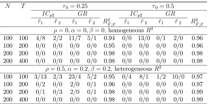
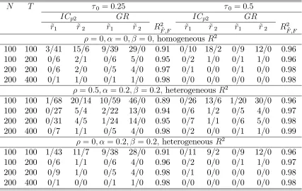
Tables 1-3 report the percentage of underestimation and overestimation of r~1,

~

r2 and averages of R2_{F ;F}^ over 1,000 replications. x=y denotes that the frequency

of underestimation and overestimation is x% and y% respectively. On the whole, the performance of ICp2 and GR are similar. If we choose the better one in each

case, the performance of r~1 and r~2 behave quite well and in most cases close to

the their correspondents based on the true change point k0. For Setups 1 and 3,

(N; T) = (100;200) is large enough to guarantee good performance in all cases. For the case 0 = 0:5, (N; T) = (100;100) is large enough. Note that for Setup 3, even

with a small magnitude of changea= 0:2, r~1 and r~2 still perform well. For Setup 2,

(N; T) = (100;200)is large enough in all cases, except for the case with = 0:5. The performance ofR2

~

F ;F is good for all cases.

Comparing the results of 0 = 0:5with 0 = 0:25and = 0with = 0:5 in each

table, we can see that the deterioration pattern is in accord with that of k~. This is not surprising since in the current setup, the estimation error ink~ is the main cause of misestimating r~1 and r~2. For r~1, underestimation of k0 decreases the size of the

pre-break subsample while overestimation increases the tendency of overestimatingr1.

Comparing Tables 2 and 3, we can see that underestimation is less harmful. Finally, it is worth noting that there is still room for improvement of …nite sample performance of r~1, r~2, either through improving the performance of ~k or through choosing an

estimator more robust to misspeci…cation of change point among all estimators of the number of factors in the literature.

9

Figure 1: Histogram of ~k for (N; T) = (100;100);(r1; r2; r+q1) = (3;5;7)

( ; ; ) = (0;0;0); homogeneousR2_, 0 = 0:25; ave(~r) = 5:68; sd(~r) = 0:60

( ; ; ) = (0;0;0); homogeneousR2_, 0 = 0:5; ave(~r) = 6:85; sd(~r) = 0:38

( ; ; ) = (0:5;0:2;0:2); heterogeneous

R2_,

0 = 0:25; ave(~r) = 5:75; sd(~r) = 0:58

( ; ; ) = (0:5;0:2;0:2); heterogeneous

R2_,

0 = 0:5; ave(~r) = 6:74; sd(~r) = 0:48

Figure 2: Histogram of ~k for (N; T) = (100;100);(r1; r2; r+q1) = (3;3;5); a= 1

( ; ; ) = (0;0;0); homogeneousR2_, 0 = 0:25; ave(~r) = 4:51; sd(~r) = 0:56

( ; ; ) = (0;0;0); homogeneousR2_, 0 = 0:5; ave(~r) = 5:00; sd(~r) = 0

( ; ; ) = (0:5;0:2;0:2); heterogeneous

R2_,

0 = 0:25; ave(~r) = 4:86; sd(~r) = 0:35

( ; ; ) = (0:5;0:2;0:2); heterogeneous

R2_,

0 = 0:5; ave(~r) = 5:00; sd(~r) = 0

Figure 3: Histogram of k~ for(N; T) = (100;100);(r1; r2; r+q1) = (3;3;5); a= 0:2

( ; ; ) = (0;0;0); homogeneousR2_, 0 = 0:25; ave(~r) = 4:27; sd(~r) = 0:60

0 = 0:5;( ; ; ) = (0;0;0); homogeneous

R2_{, ave(~r) = 4:85; sd(~r) = 0:36}

( ; ; ) = (0:5;0:2;0:2); heterogeneous

R2_,

0 = 0:25; ave(~r) = 5:60; sd(~r) = 1:17

( ; ; ) = (0:5;0:2;0:2); heterogeneous

R2_,

0 = 0:5; ave(~r) = 5:94; sd(~r) = 1:08

Table 1: Estimated number of pre-break and post-break factors and estimated factor space for setup 1 withr1 = 3; r2 = 5; r+q1 = 7

N T 0 = 0:25 0 = 0:5

ICp2 GR ICp2 GR

~

r1 r~2 r~1 ~r2 R_{F ;F}2~ r~1 r~2 r~1 r~2 R2_{F ;F}~

= 0; = 0; = 0;homogeneous R2

100 100 4/8 2/2 11/7 5/1 0.94 0/0 13/0 0/1 2/0 0.96 100 200 0/0 0/0 0/0 0/0 0.95 0/0 0/0 0/0 0/0 0.96 200 200 0/0 0/0 0/0 0/0 0.98 0/0 0/0 0/0 0/0 0.98 200 400 0/0 0/0 0/0 0/0 0.98 0/0 0/0 0/0 0/0 0.98

= 0:5; = 0:2; = 0:2; heterogeneousR2

100 100 3/13 2/3 23/4 5/2 0.95 0/4 8/1 1/2 10/0 0.97 100 200 0/2 0/0 2/0 0/1 0.96 0/0 0/0 0/0 0/0 0.97 200 200 0/1 0/3 2/0 0/1 0.98 0/0 0/0 0/0 0/0 0.99 200 400 0/0 0/0 0/0 0/0 0.98 0/0 0/0 0/0 0/0 0.99

Notes: Number of factors in each regime is estimated using ICp2 in Bai and Ng (2002) and GR

in Ahn and Horenstein (2013). x/y denotes the frequency of underestimation and overestimation is

Table 2: Estimated number of pre-break and post-break factors and estimated factor space for setup 2 withr1 = 3; r2 = 5; r+q1 = 5

N T 0 = 0:25 0 = 0:5

ICp2 GR ICp2 GR

~

r1 r~2 r~1 r~2 R2_{F ;F}~ r~1 r~2 r~1 r~2 R2_{F ;F}~

= 0; = 0; = 0;homogeneous R2

100 100 3/41 15/6 9/39 29/0 0.91 0/10 18/2 0/9 12/0 0.96 100 200 0/6 2/1 0/6 5/0 0.95 0/2 1/0 0/1 1/0 0.96 200 200 0/6 2/0 0/5 4/0 0.97 0/1 0/0 0/1 0/0 0.98 200 400 0/1 1/0 0/1 1/0 0.98 0/0 0/0 0/0 0/0 0.98

= 0:5; = 0:2; = 0:2; heterogeneousR2

100 100 1/68 20/14 10/59 46/0 0.89 0/26 13/6 1/20 30/0 0.96 100 200 0/27 5/4 2/22 13/0 0.94 0/6 1/2 0/5 4/0 0.97 200 200 0/31 4/5 1/24 14/0 0.95 0/7 1/1 0/6 5/0 0.98 200 400 0/7 1/1 0/5 4/0 0.98 0/2 0/0 0/1 1/0 0.99

= 0; = 0:2; = 0:2; heterogeneousR2

100 100 1/43 11/7 9/38 28/0 0.91 0/11 9/2 0/9 12/0 0.96 100 200 0/6 1/1 0/6 4/0 0.96 0/2 0/0 0/1 1/0 0.97 200 200 0/9 1/0 0/5 4/0 0.98 0/1 0/0 0/0 0/0 0.98 200 400 0/1 0/0 0/1 1/0 0.98 0/0 0/0 0/0 0/0 0.98

Notes: Number of factors in each regime is estimated using ICp2 in Bai and Ng (2002) and GR

in Ahn and Horenstein (2013). x/y denotes the frequency of underestimation and overestimation is

Table 3: Estimated number of pre-break and post-break factors and estimated factor space for setup 3 withr1 = 3; r2 = 3; r+q1 = 5

N T 0 = 0:25 0 = 0:5

ICp2 GR ICp2 GR

~

r1 r~2 r~1 r~2 R2_{F ;F}~ r~1 ~r2 ~r1 r~2 R2_{F ;F}~

= 0; = 0; = 0;homogeneous R2_{, a= 1}

100 100 5/4 0/1 14/0 0/1 0.97 0/0 0/0 0/0 0/0 0.97 100 200 0/0 0/0 1/0 0/0 0.97 0/0 0/0 0/0 0/0 0.97 200 200 0/0 0/0 0/0 0/0 0.98 0/0 0/0 0/0 0/0 0.99 200 400 0/0 0/0 0/0 0/0 0.99 0/0 0/0 0/0 0/0 0.99

= 0:5; = 0:2; = 0:2; heterogeneousR2,a = 1

100 100 3/9 0/8 27/0 0/4 0.97 1/4 0/4 2/1 1/2 0.97 100 200 0/2 0/4 4/0 0/2 0.98 0/1 0/0 0/0 0/0 0.98 200 200 0/1 0/3 2/0 0/2 0.99 0/0 0/0 0/0 0/0 0.99 200 400 0/0 0/1 1/0 0/1 0.99 0/0 0/0 0/0 0/0 0.99

= 0; = 0; = 0;homogeneous R2_{, a= 0:6}

100 100 4/3 0/1 12/0 0/0 0.97 0/0 0/0 0/0 0/0 0.97 100 200 0/0 0/0 1/0 0/0 0.97 0/0 0/0 0/0 0/0 0.97 200 200 0/0 0/0 0/0 0/0 0.99 0/0 0/0 0/0 0/0 0.99 200 400 0/0 0/0 0/0 0/0 0.99 0/0 0/0 0/0 0/0 0.99

= 0:5; = 0:2; = 0:2; heterogeneousR2_{, a= 0:6}

100 100 3/9 0/6 26/0 0/3 0.98 1/2 0/3 2/2 2/2 0.98 100 200 0/2 0/3 3/0 0/1 0.98 0/1 0/1 0/0 0/0 0.98 200 200 0/1 0/3 2/0 0/1 0.99 0/0 0/0 0/0 0/0 0.99 200 400 0/0 0/1 1/0 0/1 0.99 0/0 0/0 0/0 0/0 0.99

= 0; = 0; = 0;homogeneous R2_{, a= 0:2}

100 100 5/8 0/1 18/0 2/0 0.97 0/0 0/0 0/0 1/0 0.97 100 200 2/5 3/7 10/0 16/0 0.97 0/1 1/0 2/0 1/0 0.97 200 200 0/0 0/0 1/0 0/0 0.99 0/0 0/0 0/0 0/0 0.99 200 400 0/0 0/0 0/0 0/0 0.99 0/0 0/0 0/0 0/0 0.99

= 0:5; = 0:2; = 0:2; heterogeneousR2_{, a= 0:2}

100 100 5/13 0/0 33/0 0/0 0.98 1/2 1/2 3/0 2/0 0.98 100 200 1/3 0/0 7/0 4/0 0.98 0/0 0/0 0/0 1/0 0.98 200 200 0/2 0/0 3/0 0/0 0.99 0/0 0/0 0/0 0/0 0.99 200 400 0/0 0/0 1/0 0/0 0.99 0/0 0/0 0/0 0/0 0.99

Notes: Number of factors in each regime is estimated using ICp2 in Bai and Ng (2002) and GR

in Ahn and Horenstein (2013). x/y denotes the frequency of underestimation and overestimation is

point is Op(1). The main appeal of this estimator is that it does not require prior

information of the number of factors and observability of the factors and it allows for a change in the number of factors. Based on this change point estimator, we are able to dissect the model into two separate stable models and establish consistency of the estimated pre and post-break number of factors and convergence rate of the estimated pre and post-break factor space. These results provide the foundation for subsequent analysis and applications.

A natural step is to derive the limiting distribution of the estimated factors, factor loadings and common components as in Bai (2003). It will also be rewarding to further improve the …nite sample performance of our change point estimator. In addition, following the methods in Bai and Perron (1998), it will be straightforward to extend our results to the case with multiple changes. Many other issues are also on the agenda. For example, what are the asymptotic properties of the estimated change point, estimated number of factors and estimated factors when the factor process is I(1)?

References

[1] Ahn, S.C., Horenstein, A.R., 2013. Eigenvalue ratio test for the number of factors. Econometrica 81, 1203–1227.

[2] Bai, J., 1994. Least squares estimation of shift in linear processes. Journal of Time Series Analysis 15, 453–472.

[3] Bai, J., 1997. Estimation of a change point in multiple regression models. Review of Economics and Statistics 79, 551–563.

[4] Bai, J., 2003. Inferential theory for factor models of large dimensions. Economet-rica 71, 135–173.

[6] Bai, J., Ng, S., 2002. Determining the number of factors in approximate factor models. Econometrica 70, 191–221.

[7] Bai, J., Perron, P., 1998. Estimating and testing linear models with multiple structural changes. Econometrica 66, 47-78.

[8] Banerjee, A., Marcellino, M., Masten I., 2008. Forecasting macroeconomic vari-ables using di¤usion indexes in short samples with structural change. Emerald Group Publishing Limited 3, 149-194.

[9] Bates, B., Plagborg-Moller, M., Stock, J.H., Watson, M.W., 2013. Consistent factor estimation in dynamic factor models with structural instability. Journal of Econometrics 177, 289–304.

[10] Bernanke B., Boivin, J., Eliasz, P., 2005. Factor augmented vector autoregression and the analysis of monetary policy. Quarterly Journal of Economics 120, 387– 422.

[11] Breitung, J., Eickmeier, S., 2011. Testing for structural breaks in dynamic factor models. Journal of Econometrics 163, 71–84.

[12] Chen, L., 2015. Estimating the common break date in large factor models. Eco-nomics Letters 131, 70-74.

[13] Chen, L., Dolado, J., Gonzalo, J., 2014. Detecting big structural breaks in large factor models. Journal of Econometrics 180, 30–48.

[14] Cheng, X., Liao, Z., Schorfheide, F., 2015. Shrinkage estimation of high-dimensional factor models with structural instabilities. Review of Economic Stud-ies, forthcoming.

[15] Corradi, V., Swanson, N.R., 2014. Testing for structural stability of factor aug-mented forecasting models. Journal of Econometrics 182, 100–118.

[17] Leeb, H., Pötscher, B.M., 2005. Model selection and inference: Facts and …ction. Econometric Theory 21, 21-59.

[18] Lewbel, A., 1991. The rank of demand systems: theory and nonparametric Es-timation. Econometrica 59, 711–730.

[19] Moon, H.R., Weidner, M., 2015. Linear regression for panel with unknown num-ber of factors as interactive …xed e¤ects. Econometrica 83, 1543-1579.

[20] Onatski, A., 2009. Testing hypotheses about the number of factors in large factor models. Econometrica 77, 1447–1479.

[21] Onatski, A., 2010. Determining the number of factors from empirical distribution of eigenvalues. Review of Economics and Statistics 92, 1004–1016.

[22] Ross, S., 1976. The arbitrage theory of capital asset pricing. Journal of Finance 13, 341–360.

[23] Stock, J.H., Watson, M.W., 2002a. Forecasting using principal components from a large number of predictors. Journal of American Statistical Association 97, 1167–1179.

[24] Stock, J.H., Watson, M.W., 2002b. Macroeconomic forecasting using di¤usion indexes. Journal of Business and Economic Statistics 20, 147-162.