1
A Multi-Body Dynamics based numerical
modelling tool for solving biomimetic problems
Ruoxin Li1, Qing Xiao1*, Yuanchuan Liu1, Jianxin Hu2, Lijun Li3, Gen Li4, Hao Liu3,4, Kainan Hu5, Li Wen5
1Department of Naval Architecture, Ocean and Marine Engineering, University of Strathclyde, Glasgow, UK
2Faculty of Mechanical Engineering and Automation, Zhejiang Sci-Tech University, Hangzhou, China
3Shanghai Jiao Tong University and Chiba University International Cooperative Research Centre (SJTU-CU ICRC), Shanghai Jiao Tong University, Shanghai, China 4Graduate School of Engineering, Chiba University, Chiba, Japan
5School of Mechanical Engineering and Automation, Beihang University, Beijing, China
*Corresponding author: [email protected]
Keywords: multibody system, self-propulsion, unsteady locomotion, Computational Fluid Dynamics, biomimetics
Abstract
In this paper, a versatile Multi-Body Dynamic (MBD) algorithm is developed to integrate an incompressible fluid flow with a bio-inspired multibody dynamic system.
2 1. Introduction
Fish have evolved excellent propulsive and manoeuvring abilities that have allowed
them to adapt to the aquatic environment and survive the natural selection process. For
humans, the physical and biological mechanisms observed in swimming fish are a precious source of inspiration for the development of artificial swimming machines
such as Autonomous Underwater Vehicles (AUV) [1; 2].
Generally, there are two effective ways to study fish swimming mechanisms, namely
through experimental study and simulation. These methods are well summarised in
several comprehensive review papers [3-7]. The experimental approach observes and
measures the locomotion of live or robotic fish, and providesthe most reliable data for analysis and direct evaluation of the robots [8-13]. Benefitting from newly developed measuring techniques, the experimental approach can directly record fluid motion via PIV measurement [14; 15]. However, some other key physical parameters which are
beyond the capability of experimental records remain unresolved (such as the surface
stress of a swimming fish). While an experimental approach can deal with the morphological, behavioural and environmental complexities in nature, these
complexities sometimes hinder researches’ ability to arrive at mathematical principles.
To compensate for these experimental tests, computational approaches have been
adopted. The approaches can be divided into analytical models and Computational Fluid Dynamics (CFD) models. The analytical model reduces the complexity of live fish swimming during the modelling process, considering that a swimming fish is in quasi-steady state. As such, this method concentrates on the primary fluid dynamic characteristics while neglecting secondary effects (e.g. Lighthill’s Elongated Body
3
Up-to-date Computational Fluid Dynamics (CFD) models can complement the role of experimental and analytical models but are also capable of executing independent missions. In all research and engineering areas concerning fluid dynamics, CFD model predictions have been validated against experimental observations to demonstrate their accuracy.
Distinct from a traditional CFD arrangement via fixing a swimming object in an
incoming flow condition (equivalent to a water-tunnel experiment, commonly used in some commercial CFD software), present fish CFD simulations tend to allow the fish propelling themselves through water (free-swimming) [18-20]. While the self-propelling (free-swimming) arrangement requires additional coupling of hydrodynamics and body-dynamics, this method has several significant advantages.
For example, the swimming speed is no longer treated as a known input beforehand,
and thus the predicted CFD results are able to explore the kinematic and morphological parameter map beyond experimental observation (e.g. [17]). In addition, the CFD studies do not need to be limited to any stable forward motion, instead it can be expanded to various unstable or manoeuvre situations (e.g. [21; 22]).
Apart from the above-mentioned advantages, the complexity of the CFD objectives in this study have been significantly improved. Traditionally, with the increase of complexity, the studies on fish swimming can be classified into three major groups: (a) fish body undulation without considering the influence of fins; (b) single fin, such as caudal fin or multiple fins ignoring the fish body; and (c) a combined fish body with multiple fins. A brief review of the studies in the relevant areas are given in the following section.
For the first category, typical modes such as anguilliform and carangiform are introduced [5]. The anguilliform swimmer, such as the eel, bends its body into a wave shape, with the wave propagating from the fish head to the tail. To analyse this problem, a fish body can be modelled either through a continuous body or a multi-body system with several discrete elements connected via joints. Typical examples include the work from Kern and Koumoutsakos [18], Carling et al. [19] and Eldredge [23]. The carangiform mode fish, unlike the anguilliform mode, undulates the last third portion
of their body along with a caudal fin. The relevant studies can be found from the papers
4
In contrast to the first category focusing on a fish body, some numerical investigations concentrated on the performance of a single fish fin or of a fin-fin interaction (single fin: [27; 28]; passively deformable fin: [29]; rayed fin: [30; 31]; and fin-fin interaction: [32; 33]).
Apart from the above two groups, other researchers investigated a combined model for a fish with lateral (paired fins such as pectoral fins) or median fins (unpaired fins such as dorsal, anal and caudal fins). Borazjani [34] examined the function of median fins during C-start by reconstructing the model with/without fins using an Immersed Boundary Method. Their results concluded that the anal and dorsal fins played a more significant role in the stability of the fish during C-start mode than in producing hydrodynamic propulsion force. However, although the fins moved with the body of fish, their individual undulation was not considered in this study. Similarly, using an IBM method, Han et al. [35] investigated the dorsal and anal fins of a sunfish model during a cruising condition. It was found that with dorsal, anal and caudal fins, the fish has a greater efficiency compared to other conditions with only two fins. The deformation of fins was imposed by prescribing the kinematic motion, and a constant incoming velocity was given rather than as a result of fluid-structure interaction modelling. Xu and Wan [36] numerically simulated a self-propelled fish swimming with a pair of rigid pectoral fins using a multi-block and overset grid method. The rowing, feathering and flapping motions of the fins were investigated. Numerical results showed that during the turning motion, both hydrodynamic moment and lateral force were generated by the fins. The deformation of the pectoral fins was not included in this work.
5
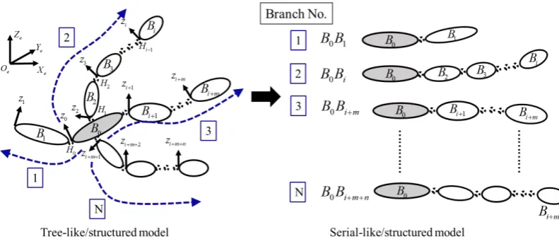
[image:5.595.99.495.194.363.2]1. A reference body B0 is selected and used as a starting element for both models. The primary difference between the two models is that, in a serial-like model, the nth element is the terminal body, whereas, a tree-like model has more than one terminal body. As demonstrated in Figure 1, several branches exist in a tree-like model and each branch can be treated as a serial-like model.
Figure 1. Sketch of Multi-Body tree-like and serial-like model. The tree-like model has one reference body (as coloured in grey) and more than one terminal body
(B B B1, i, i m+ ,Bi m n+ + ). The serial-like model has only one reference body and one terminal body. A tree-like model can be treated as composing of several branches of
serial-like models and all the branches share one reference body.
The present study succeeds and improves on the research of Hu [38; 39], whereby a serial-like MBD solver, based on a hybrid Mobile Multi-Body algorithm [40-42] is
6
To describe this new model and validate its capability, the remainder of the paper is structured as follows. Section 2 will introduce in detail the tree-like Multi-Body Dynamics algorithm, the fluid solver and the coupling between the two. Section 3 will present four canonical examples to illustrate the application of our developed numerical tool, including the comparison with some available experimental and CFD results. This will cover a discrete eel-like model, a continuous eel-like body, a peduncle-caudal-fin and a self-propelled fish swimming induced by its multiple fin undulation.
2. Numerical methods
In this section, detailed description on the established numerical methodology will be introduced. The fluid flow around fish and fins is solved using Commercial software ANSYS Fluent 15.0. To cope with the complex body and multiple rigid and/or deformable fins locomotion, as explained fully in Section 2.1, dynamics of the model
are solved using Multi-Body tree-like algorithms. This part is developed with an in-house code and embedded into User Defined Function (UDF) of ANSYS Fluent. At each time step, data exchange occurs between the fluid solver and the in-house code. 2.1. Multi-Body Dynamics algorithm
The biomimetic problem to be solved is complicated and can include multiple degrees of freedom related locomotion of a fish body, such as translation and rotation. Fish forward motion induced by the undulation of the body or fins is also one of the numerical FSI solutions. In addition, fish fins may undergo independent locomotion, which is different from the main body. It is thus very challenging to use traditional rigid body dynamics to solve this problem. To cope with this, the dynamics of the model is handled by a Multi-Body Dynamics method based on previous work [9; 39; 40]. Primarily, at each time step, the fluid force applied on each element/body in the MBD model is obtained from the fluid solver and passed to our in-house code. The overall force on the entire model is the accumulation of all relevant elements. With the use of Newton’s Second Law, the entire dynamic model acceleration is determined. By integrating once and twice with time, the velocity and location relative to the global coordinate is obtained, respectively. The above process always starts with a specified reference body (see Figure 1), then to each element along different branches based on
7 2.1.1. Model description
The whole model is considered as being constructed with several separate elements/bodies as given in Figure 1. These elements can be either rigid or deformable. In the present algorithm, the deformation of elements is achieved by prescribing the motion at each grid point on the surface of elements. There are two types of coordinate in this system, i.e. global coordinate Oe and local coordinates Oi. The reference body
0
B is specified and coloured in grey. Several branches exist, indicated by blue arrow
dashed lines, relative to the reference body B0. Apart from the reference body B0,
other elements in the branches are given numbers in the orders of 1 to the last element. Two adjacent elements are connected with one virtual hinge Hi. At each hinge, there
is only one degree of freedom motion that can be imposed, i.e. rotational motion about local z axis. By adding more than one virtual hinge, multi-degrees of freedoms can be achieved. For the model consisting of rigid elements, prescribed rotational acceleration
can be provided at each hinge so that within one time step the angular velocity and angle i at each hinge is known. In terms of a system with deformable elements, the hinge motion is zero, i.e. there is no relative rotational motion between two adjacent elements connected by the hinge. An index vector a is employed to store element/body connection information, which is vital for a tree-like MBD system. 2.1.2. Euler transformation
Transformation between two successive local coordinates is completed based on the
Newton-Euler Frame. A homogeneous transformation matrix j i
T which transforms the initial location/position from a local coordinate of body B O x y zi( , , , )i i i i to
( , , , )
j j j j j
B O x y z is defined as:
rot( , )trans( , )rot( , )trans( , )
cos sin 0
cos sin cos cos sin sin
sin sin sin cos cos cos
0 0 0 1
= − − − = − j
i i j j j j
j j j
j j j j j j j
j j j j j j j
x x d z q z r
q q d
q q r
q q r
T
8
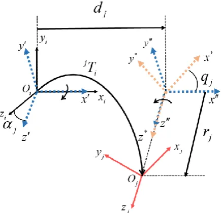
[image:8.595.187.405.214.424.2]Referring to Figure 2, transformations operate along the x and z axis in order. The local coordinate of body B O x y zi( , , , )i i i i firstly rotates around the xi axis with an angle of j , translates along the x axis with a distance of dj, then rotates about the
z
axis with an angle of qj, and translates along z* axis with the distance rj to get the final local coordinate of body B O x y zj( j, j, j, j).Figure 2. Coordinate transformation: transformation matrix j i
T from local coordinate i
O of body Bi to the local coordinate Oj of body Bj
When the angular motions
a on the hinge connecting two consecutive bodies is specified, the transformation matrix jTi(a) is divided into one (3 3 ) rotationmatrix jRi(a) and one (3 1 ) position vector j i P as:
( ) rot( , )trans( , )rot( , )trans( , ) ( )
0 1
= +
=
j
i a i j j j a j
j j
i a i
x x d z q z r
T
R P (2)
The angle
a is determined by looking through the index vector a. An adjoint map operator ji g
9
ˆ
( ) ( )
0 ( )
= j i
j j i T
i a i a j
g j
i a
Ad R R P
R (3)
ˆ
i j
P is a (3 3) skew-symmetric tensor and can be obtained from the (3 1 )
position vector i j P .
2.1.3. Force and acceleration
The fluid force of each element is obtained by fluid solver at each time step and notated as a (6 1 )force vectorFext j, , including force and moment in three directions. The net
force
j on the terminal body is defined as:
,
= −
j j Fext j (4)
where j is a (6 1) Coriolis and centrifugal forces vector. For detailedderivation, refer to Porez et al. [9]. The inertia tensor j consists of a (3 3) tensor of body massMj, two (3 3) tensors of first inertia moments MSˆj and a tensor of angular
inertia Ij:
ˆ ˆ − = j j j j j M MS
MS I (5)
As body Bi is followed by bodyBj, the inertia tensor and force between these two bodies is linked by the following equations:
* * , ( ) ( ( ) ) = + = − + + + i i j j i j T
i i g j g
T
i i ext i g j j j j
Ad Ad
F Ad A (6)
10
By accumulating the force and inertia tensor from the terminal body back to the reference body, the acceleration 0 of reference bodyB0 in the local coordinate can be estimated as:
1
0 ( 0) 0
= − − (7)
2.1.4. Velocity and position
The status of the whole system relative to the earth coordinate is decided by the reference bodyB O x y z0( 0, 0, 0, 0) . Its velocity
0 in the local coordinate is solved using the 4th order Runge-Kutta scheme as follows:1 2 3 4
0 1
0 1 0 0 0 0 0
2 2 0 1 2 2 6 t t t
t t t t t t t
t V t + + + + + + = = + + + +
(8)
where V0 and 0 represent a (3 1 ) linear vector and a (3 1 ) angular velocity
vector in the x, y, z direction. The velocity 0 of the reference body in the local coordinate can be transferred to the earth coordinate as:
0 0 0
e e
R
= (9)
where e 0
R is a
(
3 3)
matrix associated with the orientation of the reference body. With a(
3 1)
position vector 0e
P , the transformation matrix e 0
T between the earth coordinate and the reference body is:
0 0 0 0 1 = e e
e R P
T (10)
Velocity for the other bodies is calculated recursively from the reference body forward to the terminal body. The transformation of velocity
from an anterior body Bi toits following body Bj is defined as:
, (11)
11
The position of other bodies relative to the global coordinate is also obtained by transforming from the reference body forward to the terminal body using the following equation: ( ) 0 1 = =
e e i
j i j a
e e
j j
R P
T T T
. (12)
where e i
T and e j
T are the transformation matrices for bodies Bi and Bj ;
e j
R
and e j
P are the orientation matrix and position vector of body Bj. All the variables are in the earth coordinate.
2.2. Fluid Solver
As mentioned earlier, the fluid flow around fish and fins are solved using ANSYS Fluent, a Finite Volume Method (FVM) CFD tool. The governing equations are incompressible continuity and momentum equations:
(
)
1 20 + = − + = u
u u p u
t u
(13)
where u=( , , )u v w is the fluid velocity vector, p is the fluid pressure,
is the fluid12
Due to the large deformation of the mesh when fish swim, the dynamic mesh function available in Fluent is used. As a body in the Multi-Body system could be considered as either rigid or deformable, different forms of User Defined Functions are used for the dynamic mesh zones. Given rigid bodies, the velocity of each body should be imported to Fluent. As for deformable bodies, the position of every mesh node on the deformable body surface is calculated in the MBD code and given to Fluent at each time step. These variables are relative to the global coordinate.
2.3. Coupled algorithm
At each time step, the transfer of data is needed between the fluid solver and UDF. At the beginning of each time step, the velocity and position of each body relative to the global coordinate is transferred to Fluent to calculate the fluid force around the model. Such information is then delivered back to the MBD code to predict the velocity and position of the fish at the next time step.
A vector
(
Xstate, j, j)
collects the status Xstate of reference body B0, the angular velocity and the angle j of all the hinges, j in total, in a model:(
, ,) (
0, 0, 0, 0, ,)
= e e e e
state j j j j
X V P Q (14)
Generally, to predict a new time step, a 4th order Runge-Kutta explicit time discretization is employed as:
(15)
Here, t stands for time step size.
3. Case studies
13
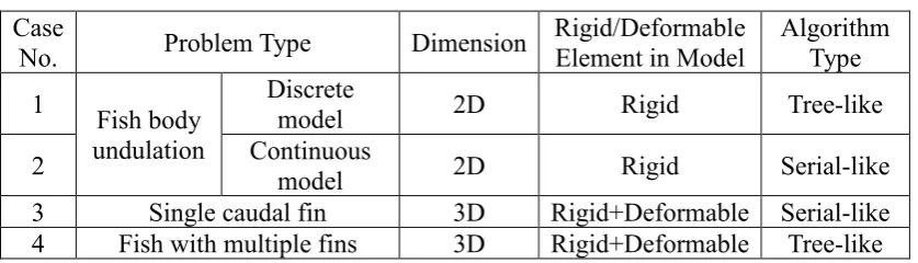
Table 1 Summary of the case studies Case
No. Problem Type Dimension
Rigid/Deformable Element in Model
Algorithm Type 1 Fish body
undulation
Discrete
model 2D Rigid Tree-like
2 Continuous model 2D Rigid Serial-like
3 Single caudal fin 3D Rigid+Deformable Serial-like 4 Fish with multiple fins 3D Rigid+Deformable Tree-like 3.1. Discrete fish body undulation
In the previous work of Eldredge [23], a two-dimensional model made of three identical rigid elements was investigated to simulate a simplified undulation motion of an
anguilliform free-swimming fish. This can be considered as splitting a continuous eel-like fish body into several separate elements connected by joints. The geometric shape of each element is ellipse, with an aspect ratio of major vs. minor axis of 10. The length of each element is a, and the distance d between each body is 0.2a. To use our MBD method, the middle body is selected as the reference bodyB0, the other two bodies, numbered asB1 andB2 , are treated in two different branches. The local coordinate system for each body is illustrated in Figure 3. In order to obtain comparable results with the previous study, the rotational angular motions (1 and
2 ) are specified between two adjacent bodies (B0 and B1, B0 and B2) as:1
2
( ) cos( ) 2 ( ) cos( )
= −
= −
t t
t t
(16)
[image:13.595.153.452.514.699.2]14
An undulation Reynolds number [23] is used in the present study and is equal to 200 via the following equation:
(17)
where is the maximum angular velocity, a is the length of each ellipse, and is the kinematic viscosity.
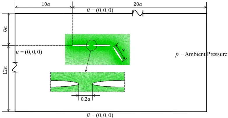
The computation is performed in a domain with a size of 30a20a, shown in Figure
4, which is large enough to avoid the boundary influence. The model is placed 10a
and 8a away from the inlet and upper boundary, respectively. Around the model, a small inner zone is designed to better capture the vortex structure around the swimming body. Unstructured triangular meshes are applied to the whole computational domain and the overall grid number is around 141,000. At the surface of the three elements, no slip boundary conditions are imposed. A constant velocity (u=(0, 0, 0)) are set to the
left, upper and lower boundary and the pressure at the right boundary is set to ambient pressure. Time step is set as
500
[image:14.595.104.495.457.660.2] =t T after testing, where T is the undulating period.
15 (a) Rotational motion
(b) X direction
[image:15.595.80.536.74.531.2](c) Y direction
Figure 5 Velocity and Displacement comparisons between Eldredge [23] and present study on the rotational motion, X and Y direction of the reference body
16
negative for V, and hence the undulating fish moves towards the positive X and negative Y direction. Meanwhile, the displacement in the Y direction is smaller and more oscillated than that in the X direction. For rotational motion, the rotational angle varies from an approximate -0.8 rad to 0.2 rad.
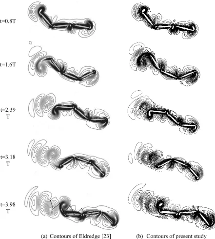
t=0.8T
t=1.6T
t=2.39 T
t=3.18 T
t=3.98 T
[image:16.595.55.497.164.655.2]17
can be observed in the downstream of the model. Overall a good comparison with the
previous study is clearly demonstrated.
The successful validation of applying our MBD algorithm to this discrete model is vital in the bio-inspired robot area, as most anguilliform robot fish are made of a series of modules with motion control actuators placed between two adjacent modules, such as
AmphiBot III [9].
3.2. Continuous Anguilliform fish undulation
To demonstrate that the established MBD is also applicable to modelling continuous body locomotion like an anguilliform mode, a two-dimensional self-propelled eel-like fish model is selected in this section, which is taken from Carling et al. [19].
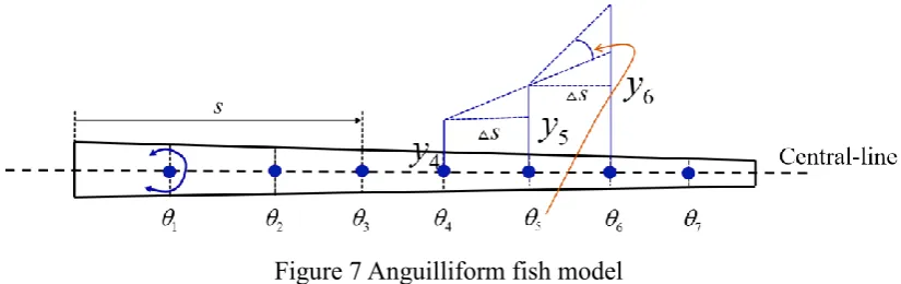
The model is constructed using eight trapezoidal bodies, as shown in Figure 7. The length s of each body at initial time is identical. Based on the geometry provided by Carling et al. [19], the total fish length l is 0.08m. The width of the whole model is defined as:
2 2
0.0064 0.0048(3 2 / )
= − −
n n n
w s l s l (18)
[image:17.595.92.505.511.641.2]where sn stands for the distance from the fish head to the current hinge location (nth). The widest length of the model w is at the fish head with a value of 0.0064m.
Figure 7 Anguilliform fish model
At the onset, there is no bending of the fish body, thus its central line is a straight line. Previous studies used a prescribed central line kinematic undulating motion to drive the fish to move forward. The vertical linear motion of the central line was described as:
/ 0.25
sin[( / ) 2 / ]
1.25
+
= n −
n n
s l
18
where yn stands for the vertical movement of the central line at location sn [19]. Simulation is carried out at a specific period T of 1.2s.
To use the present MBD algorithm, the central line motion is converted to a series of angular motions imposed at each virtual hinge. The angular motion on hinge n is determined by three successive vertical movementyn+1, yn and yn−1 at the location of sn+1, sn and sn−1, respectively, which is indicated in Figure 7 and described by the following equation:
1 1
arctan arctan
= n+ − n − n− n−
n
y y y y
s s (20)
The variable
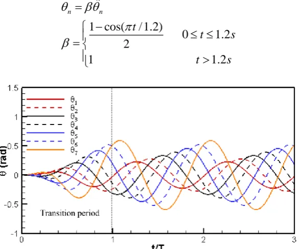
n is the angular motion on the nth hinge and is given as a known variable into the MBD algorithm. A transition function , as shown in Eq. (21), is utilised in the first undulation period to ensure the angle increases gradually such that no break-down of the iteration could occur due to a dramatic change of angle. Figure 8 displays the prescribed angular motion profiles
n at all seven hinges within the first cycle - a transition cycle as discussed above.ˆ
1 cos( / 1.2)
0 1.2 2
1 1.2
= −
=
n n
t
t s
t s
[image:18.595.152.445.453.696.2](21)
19
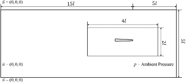
The simulation is carried out in a domain as presented in Figure 9. The model is placed 5l away from the outlet boundary. The whole domain is split into inner and outer zones to ensure good mesh quality around the model. No slip boundary is set on the surface of the fish. The pressure at the downstream boundary is given as ambient pressure. The other three boundaries are set as constant velocity (u=(0, 0, 0)). The mesh in the entire
domain is triangular mesh. A time step of
300
= T
[image:19.595.105.491.231.404.2]t is selected for the simulation.
Figure 9 Computational domain of anguilliform fish
Figure 10 shows the forward and lateral velocity comparisons with Carling et al. [19].
It is clear that our results compare well with the previous study. As the first undulating
period is taken as a transition stage, only the body shape is modified. Thus, the FSI induced forward velocity remains at zero and there is no translational motion of the fish. From the second period onwards, the fish begins to accelerate and then reaches a quasi-stable status.
The vorticity field of the fish swimming within 15 undulating periods is plotted in Figure 11 with the existence of a typical reversed Karman Vortex structure. In one undulating period, the beating amplitude of the fish tail has two peaks indicating that
the vortex shed twice in one period.
The above comparison between our numerical results and others provides evidence that
20
Figure 10 Velocity comparisons (Blue lines: results of Carling et al. [19]; red lines: present results)
Figure 11 Vorticity contour for 15 undulating periods (z vorticity with the values from -3 to 3 in 20 intervals)
3.3. Fish peduncle-caudal cupping motion
[image:20.595.91.509.334.486.2]21
[image:21.595.103.499.78.682.2](a) Component of model (b) Sketch of experiment Figure 12 Experimental model of fish peduncle-caudal [43]
(a) Fish peduncle-caudal model (b) XZ view and caudal fin dimensions
(c) YZ view and peduncle dimensions (d) XY view and peduncle dimensions Figure 13 Fish peduncle-caudal CFD model and dimensions
22
17.5°, 27.5° and 37.5°) in Figure 13(b). The caudal peduncle is modelled as a wedged body with three dimensions (L W H ) indicated in Figure 13(c) and (d).
The computational domain, as shown in Figure 14, is large enough to minimise the influence of the outer boundaries. The model is placed
4
L
away from the inlet boundary. Two mesh zones are generated with an inner zone having unstructured tetrahedral elements and an outer zone with structured hexahedral mesh. The total mesh number is approximately 430,000 and the unsteady time step is selected as 500 steps per time period. The inlet boundary is given as a constant velocity, equal to the towing speed during the experiment, which is determined by the Strouhal number, and defined as:
= f A
St
u (22)
[image:22.595.130.466.448.636.2]where f, A and u is the frequency, translational motion amplitude and the inlet velocity respectively. The pressure at the right boundary is set to ambient pressure and the surrounding boundary is symmetry. The surface of the peduncle-caudal model is treated as a no slip boundary.
Figure 14 Sketch of fish peduncle-caudal computational domain
23
experiment, the rotational and translational motions are provided on B0, as defined in the following equations:
Translational 0.02 sin(2 )
Rotational 0.2618sin(2 ) 2
=
= −
T R
S t
A t (23)
The cupping motion of the deformable caudal fin can be treated as successive fin rays with different undulating amplitudes, given as:
( ) sin(2 )
= A t (24)
where
is the angle between each fin ray (blue line in Figure 15) and the x axis relative to its local coordinate (red line in Figure 15); A( )
is the amplitude of eachundulating fin ray, described is:
( )
21 2 3
= − +
A a a a (25)
[image:23.595.229.365.420.558.2]Detailed values of the parameters used in Eq. (25) are given in Table 2 taken from [43].
Figure 15 Definition of θ for the peduncle-caudal model Table 2 Motion parameters for the peduncle-caudal model
1
a a2 a3
16 0.4677 0.0068
Simulations are performed for four Strouhal numbers. Figure 16 compares the time averaged thrust between the experiment and CFD modelling at four St, where the thrust is defined as the total force acting on the peduncle and caudal fin in x direction:
= +
thrust peduncle caudal
24
As seen from Figure 16, the predicted results are consistent with the experiment. Within the St range tested, thrust increases with the St number. A variation of time-dependent force is displayed in Figure 17 at St=0.3 for five time periods. Negative values stand for resistance while the positive values reflect propulsion force. Clearly, as indicated by
their signs, peduncle always suffers resistance, possibly due to its blunt shape, while
[image:24.595.103.484.213.386.2]the deformable caudal fin generates propulsion force.
Figure 16 Thrust comparisons between CFD results and experiment results [43]
Figure 17 Forces on peduncle and caudal fin in x direction at St=0.3
The flow visualization on the instantaneous vortex topology in one motion cycle is shown in Figure 18 from two planes. The vortices shed from the caudal fin generate a chain of vortex rings downstream. Further, the vortex rings are linked, which agrees
[image:24.595.104.479.430.605.2]25
It should be noted that some subtle differences can be observed between the experiment and the CFD at St=0.2, 0.5. This might be caused by the caudal fin edge effect since
[image:25.595.159.453.164.680.2]it has a passive motion in the experiment, while in our CFD modelling the whole surface of the caudal fin is given a prescribed deformation extracted from experimental data.
26
The quantitative comparison between our CFD prediction and experimental data further demonstrates that the present MBD model can deal with complicated swimming locomotion, including both caudal peduncle rotational translational motions and flexible fin ray undulation.
3.4. Pufferfish with multiple deformable fins
For the sake of ensuring the feasibility of a free moving rigid-deformable Multi-Body Dynamics system, we apply our code to a self-propulsion fish problem driven by dorsal, anal and caudal fins, such that the fins are considered deformable while the fish body
is rigid.
Figure 19(a) shows the numerical model of a three-dimensional pufferfish, which is extracted from the experimental data of a live pufferfish in Figure 19(b). Detailed information about the experiment can be referred to in the paper by Li et al. [45]. It was observed in the experiment that pectoral fins have subtle movements compared to dorsal and anal fins, and hence the kinematic analysis about the pair of pectoral fins was neglected in Li et al. [45]. In order to ensure consistency with experimental observations, in the present CFD modelling, the motion of pectoral fins is excluded. However, the method developed herein is able to cope with the dynamic motion of pectoral fins as long as the kinematic data is available from the experiment.
The total length (L) of the model is approximately 0.11m and the shape of each cross-section of the fish body is close to elliptic. The maximum major and minor-axis of the body are approximately 0.04m and 0.03m, respectively. All three fish fins are modelled as wedged surfaces. The density of the fish model is assumed to be the same as that of water, i.e.fish =water , which is a reasonable assumption for major aquatic animals.
Thus, the influence of gravity and buoyancy may be ignored.
[image:26.595.312.499.628.722.2]27
[image:27.595.183.408.70.245.2](c) Coordinates setting based on the MBD tree-like algorithm Figure 19 Morphology of the pufferfish
Adopting the established Multi-Body System concept, this model is considered as a four-element system, as shown in Figure 19(c). The fish body is selected as the reference body B0 and the other three elements are connected toB0, numbered asB2,
3
B and B4 for dorsal, anal and caudal fins, respectively.
Figure 20 Definition of θ for pufferfish fins
To model the deformable fish fin, the experimentally measured kinematics are used. The experiments revealed that the dorsal and anal fins undulate in phase with each other, while there is a 180-degree (π) phase lag between the caudal fin and the other two fins. Each fin is treated as comprising of successive fin rays with a sinusoidal wave travelling from the anterior-most edge down along the fin rays [46]. No deformation along the fin span-wise direction is taken into account. The equation to describe the undulated fin surface is expressed as:
( ) sin( ( ))
=A t+ (27)
[image:27.595.226.364.383.497.2]28
frequency; A( ) and ( ) are the undulating amplitude and phase angle of each
fin ray, respectively.
For deformable dorsal and anal fins, amplitude and phase angle can be expressed as:
3 2
1 2 3 4
3 2
1 2 3 4
( ) ( ) = + + + = + + +
A a a a a
p p p p (28)
The prescribed motion of the deformable caudal fin surface can be defined as:
1 2
1 2
( ) cos( )
( ) cos( )
= + = + c a c p
A a a
p p (29)
Detailed parameters for the kinematics can be found in Table 3 and the envelopes of flexible dorsal, anal and caudal fin in one undulating period are shown in Figure 21. A time step size
500
= T
t is selected for the simulation, where T is the time period and
equals 0.192s.
Table 3 Motion parameters for pufferfish model with multiple fins Amplitude A (rad)
Dorsal Anal Caudal
a - - 6.07
1
a 0.1353 0.0066 0.3861
2
a 0.3204 0.3204 0.3204
3
a 0.3563 0.3563 -
4
a 0.8898 0.8898 -
Phase angle ψ (rad)
Dorsal Anal Caudal
p - - 3.48
1
p 0.7247 0.7247 0.7247
2
p 0.2648 0.2648 0.2648
3
p 1.473 1.473 -
4
[image:28.595.92.507.422.682.2]p 4.106 4.106 -
29
2BL/s velocity is obtained for a live fish, our CFD result (1.71BL/s) is about 14.5% underestimated. Without considering the possible deformation of the flexible fins in a span-wise direction in our CFD modelling, the predicted final induced swimming velocity is reasonable. This means that our tree-like MBD code can solve the 3D self-propelled fish with median fins.
[image:29.595.105.498.189.314.2]Dorsal Anal Caudal
Figure 21 Envelopes of flexible dorsal, anal and caudal fin in one undulation period
Figure 22 Velocity and displacement in X direction for a self-propelled pufferfish with deformable fins
Apart from the above data which is available from both experiment and CFD methods, our numerical simulation can also provide additional information which is typically
[image:29.595.103.486.352.516.2]30
2
1 2
=
f
f x
F C
u A
(30)
where
F
represents the force, f is the fluid density, ux is the time averaged velocity for steady swimming fish and A is the largest crossing area of the fish body. In Figure 23, the negative values signify that the generated forces are towards the same direction the fish are swimming. As the fish swims steadily along the negative direction of x, a negative force is a reflection of thrust force, while a positive force is an indication of the drag or resistance force. The thrust generated by the deformable dorsal and analfins are always negative, while the caudal fin produces a thrust larger than drag. The
[image:30.595.109.484.318.483.2]fish body always suffers drag while swimming.
Figure 23 Dimensionless force on the fish body, dorsal, anal and caudal fins during quasi-stable swimming
In terms of propulsion efficiency, it is defined as the mean output power over mean total input power:
= out eff
in
P P
(31)
As the pufferfish swims towards negative X direction, the output power Pout is obtained by multiplying the total propulsive forces Fpropulsion x− by the induced time averaged velocity ux during quasi-stable swimming, shown as:
− =
out propulsion x x
31
The propulsion force Fpropulsion x− is considered as being generated by dorsal Fdorsal x− , anal Fanal x− and caudal fins Fcaudal x− :
− = − + − + −
propulsion x dorsal x anal x caudal x
F F F F (33)
The total input power Pin is defined by the multiplication of the torque and the
angular velocity :
(34)
Torque is obtained by integrating the moment of pressure force along the fin’s
rotation axis over each fin surface. For the deformable fin, the averaged angular velocity
of the whole fin surface is used. The time averaged input and output power is 1.79mW and 0.8mW, respectively. Thus, the efficiency is 45.44%.
2
=
t T t=4T
6
=
t T t=8T
10
=
[image:31.595.97.472.346.721.2]t T
32
Detailed vorticity contour for deformable fins is displayed in Figure 24. It is observed that dorsal and anal fins generate vortex, as does the caudal fin. Flow visualization results reveal that apparent interactions among caudal, dorsal and anal fins can be found for deformable fins.
4. Conclusion
In this work, we presented a newly developed method to solve bio-inspired swimming problems. The locomotion of fish and fins is simulated using a Multi-Body Dynamic theory and the fluid flow field around the fish is investigated with a CFD numerical method. Four case studies were tested, including a three-linked rigid-body swimmer, one anguilliform fish model, a cupping motion of a caudal fin and a self-propelled pufferfish with dorsal, anal and caudal fins. Our research relates to previous studies on
the undulating motion of both a discrete eel-like model and a continuous eel-like body, single caudal fin oscillation and fish swimming induced by multiple fins’ undulation. Numerical results are compared with data from other available resources and good comparisons are made. We have shown that this new modelling tool can be applied to comprehensive studies on fish swimming behaviour via either the undulating or oscillating motion of both fish body and different types of rigid/deformable fins. 5. Acknowledgement
Results were obtained using the EPSRC funded ARCHIE-WeSt High Performance Computer (www.archie-west.ac.uk). EPSRC grant no. EP/K000586/1. Hao Liu is partly supported by the Grant-in-Aid for Scientific Research on Innovative Areas of No. 24120007. Kainan Hu and Li Wen are supported by the National Science Foundation, China (grant no. 61633004 and 61333016). Authors would like to acknowledge Professor Frédéric Boyer and Dr Mathieu Porez at Institut de Recherche en Communication et Cybernétique de Nantes (IRCCyN) for their initial support to our Multi-Body Dynamics development. The authors are also grateful to the UK Royal Academy Engineering for partial support of this work.
References
33
[2] Roper DT, Sharma S, Sutton R, Culverhouse P (2011). A review of developments towards biologically inspired propulsion systems for autonomous underwater vehicles. Proceedings of the Institution of Mechanical Engineers, Part M: Journal of Engineering for the Maritime Environment, 225(2), 77-96.
[3] Webb PW, The biology of fish swimming, in The Mechanics and Physiology of Animal Swimming:, L. Maddock, Q. Bone, and J.M.V. Rayner, Editors. 1994, Cambridge University Press: Cambridge. p. 45-62.
[4] Webb PW (1984). Form and function in fish swimming.Scientific American, 251, 72-82.
[5] Sfakiotakis M, Lane DM, Davies JBC (1999). Review of fish swimming modes for aquatic locomotion.IEEE Journal of Oceanic Engineering, 24(2), 237-252. [6] Lauder GV (2015). Fish locomotion: recent advances and new directions.Annual
Review of Marine Science, 7, 521-545.
[7] Liu H, Kolomenskiy D, Nakata T, Li G (2017). Unsteady bio-fluid dynamics in flying and swimming.Acta Mechanica Sinica, 33(4), 663-684.
[8] Ren Z, Hu K, Wang T, Wen L (2016). Investigation of Fish Caudal Fin Locomotion Using a Bio-inspired Robotic Model. International Journal of Advanced Robotic Systems.
[9] Porez M, Boyer F, Ijspeert AJ (2014). Improved Lighthill fish swimming model for bio-inspired robots: Modeling, computational aspects and experimental comparisons.The International Journal of Robotics Research.
[10] Drucker EG, Lauder GV (2001). Locomotor function of the dorsal fin in teleost fishes: experimental analysis of wake forces in sunfish.Journal of Experimental Biology, 204(17), 2943-2958.
[11] Drucker EG, Lauder GV (2005). Locomotor function of the dorsal fin in rainbow trout: kinematic patterns and hydrodynamic forces. Journal of Experimental Biology, 208(23), 4479-4494.
[12] Standen EM, Lauder GV (2005). Dorsal and anal fin function in bluegill sunfish Lepomis macrochirus: three-dimensional kinematics during propulsion and maneuvering.Journal of Experimental Biology, 208(14), 2753-2763.
[13] Drucker EG, Lauder GV (2000). A hydrodynamic analysis of fish swimming speed: wake structure and locomotor force in slow and fast labriform swimmers. Journal of Experimental Biology, 203(16), 2379-2393.
[14] Flammang BE, Lauder GV, Troolin DR, Strand T (2011). Volumetric imaging of shark tail hydrodynamics reveals a three-dimensional dual-ring vortex wake structure.Proceedings of the Royal Society B: Biological Sciences.
[15] Müller UK, van den Boogaart JGM, van Leeuwen JL (2008). Flow patterns of larval fish: undulatory swimming in the intermediate flow regime.Journal of Experimental Biology, 211(2), 196-205.
34
[17] Li G, Müller UK, van Leeuwen JL, Liu H (2016). Fish larvae exploit edge vortices along their dorsal and ventral fin folds to propel themselves. Journal of The Royal Society Interface, 13(116).
[18] Kern S, Koumoutsakos P (2006). Simulations of optimized anguilliform swimming.Journal of Experimental Biology, 209(24), 4841-4857.
[19] Carling J, Williams TL, Bowtell G (1998). Self-propelled anguilliform swimming: simultaneous solution of the two-dimensional Navier-Stokes equations and Newton's laws of motion.Journal of Experimental Biology, 201(23), 3143-3166. [20] Li G, Müller UK, van Leeuwen JL, Liu H (2012). Body dynamics and
hydrodynamics of swimming fish larvae: a computational study. Journal of Experimental Biology, 215(22), 4015-4033.
[21] Borazjani I, Sotiropoulos F, Tytell ED, Lauder GV (2012). Hydrodynamics of the bluegill sunfish C-start escape response: three-dimensional simulations and comparison with experimental data. The Journal of Experimental Biology, 215(4), 671-684.
[22] Li G, Müller UK, van Leeuwen JL, Liu H (2014). Escape trajectories are deflected when fish larvae intercept their own C-start wake.Journal of The Royal Society Interface, 11(101).
[23] Eldredge JD (2008). Dynamically coupled fluid–body interactions in vorticity-based numerical simulations.Journal of Computational Physics, 227(21), 9170-9194.
[24] Maertens AP, Gao A, Triantafyllou MS (2017). Optimal undulatory swimming for a single fish-like body and for a pair of interacting swimmers.Journal of Fluid Mechanics, 813, 301-345.
[25] Ogata Y, Azama T, Moriyama Y (2017). Numerical investigation of small fish accelerating impulsively to terminal speed. Journal of Fluid Science and Technology, 12(1), JFST0009-JFST0009.
[26] Curatolo M, Teresi L (2016). Modeling and simulation of fish swimming with active muscles.Journal of Theoretical Biology, 409, 18-26.
[27] Li N, Su Y (2016). Fluid Dynamics of Biomimetic Pectoral Fin Propulsion Using Immersed Boundary Method.Applied Bionics and Biomechanics, 2016, 22. [28] Zhang Y, He J, Low K-H (2013). Numeric simulation on the performance of an
undulating fin in the wake of a periodic oscillating plate.International Journal of Advanced Robotic Systems, 10.
[29] Zhu Q, Shoele K (2008). Propulsion performance of a skeleton-strengthened fin. Journal of Experimental Biology, 211(13), 2087-2100.
[30] Shoele K, Zhu Q (2009). Fluid–structure interactions of skeleton-reinforced fins: performance analysis of a paired fin in lift-based propulsion. Journal of Experimental Biology, 212(16), 2679-2690.
35
[32] Akhtar I, Mittal R, Lauder GV, Drucker E (2007). Hydrodynamics of a biologically inspired tandem flapping foil configuration. Theoretical and Computational Fluid Dynamics, 21(3), 155-170.
[33] Shoele K, Zhu Q (2015). Performance of synchronized fins in biomimetic propulsion.Bioinspiration & Biomimetics, 10(2), 026008.
[34] Borazjani I (2013). The functional role of caudal and anal/dorsal fins during the C-start of a bluegill sunfish.Journal of Experimental Biology, 216(9), 1658-1669.
[35] Han P, Liu G, Ren Y, Dong H (2016). Computational Analysis of 3D Fin-Fin Interaction in Fish’s Steady Swimming. ASME 2016 Fluids Engineering Division Summer Meeting FEDSM2016, Washington, DC, USA, FEDSM2016-7699.
[36] Xu Y, Wan D (2012). Numerical simulation of fish swimming with rigid pectoral fins.Journal of Hydrodynamics, Ser. B, 24(2), 263-272.
[37] Khalil W. Modeling and Control of Manipulators. Nantes.
[38] Hu J, Xiao Q, Nguyen VT (2013). An Exploration of a PASSIVE Articulated Fish-Like System. ASME 2013 32nd International Conference on Ocean, Offshore and Arctic Engineering, Nantes, France, OMAE2013-10808.
[39] Hu J (2016). Numerical study on hydrodynamic performance of bio-mimetic locomotion. Ph.D Thesis, University of Strathclyde, Glasgow, Scotland, UK. [40] Porez M, Boyer F, Belkhiri A (2014). A hybrid dynamic model for bio-inspired
robots with soft appendages-Application to a bio-inspired flexible flapping-wing micro air vehicle. IEEE International Conference on Robotics and Automation (ICRA'2014), Hong Kong, hal-00861321.
[41] Boyer F, Porez M (2015). Multibody system dynamics for bio-inspired locomotion: from geometric structures to computational aspects. Bioinspiration & Biomimetics, 10(2), 025007.
[42] Khalil W, Boyer F, Morsli F (2017). General Dynamic Algorithm for Floating Base Tree Structure Robots With Flexible Joints and Links.Journal of Mechanisms and Robotics, 9(3), 031003-031003-13.
[43] Hu K, Ren Z, Wang Y, Wang T, Wen L (2016). Quantitative hydrodynamic investigation of fish caudal fin cupping motion using a bio-robotic model. 2016 IEEE International Conference on Robotics and Biomimetics (ROBIO), 295-300.
[44] Lauder GV, Drucker EG (2002). Forces, fishes, and fluids: hydrodynamic mechanisms of aquatic locomotion.Physiology, 17(6), 235-240.
[45] Li L, Li G, Li R, Xiao Q, Liu H (2018). Multi-fin kinematics and hydrodynamics in pufferfish steady swimming.Ocean Engineering, 158, 111-122.
![Figure 5 Velocity and Displacement comparisons between Eldredge [23] and present study on the rotational motion, X and Y direction of the reference body](https://thumb-us.123doks.com/thumbv2/123dok_us/1393509.92473/15.595.80.536.74.531/figure-velocity-displacement-comparisons-eldredge-rotational-direction-reference.webp)
![Figure 10 Velocity comparisons (Blue lines: results of Carling et al. [19]; red lines: present results)](https://thumb-us.123doks.com/thumbv2/123dok_us/1393509.92473/20.595.91.509.334.486/figure-velocity-comparisons-blue-results-carling-present-results.webp)