City, University of London Institutional Repository
Citation
:
Albrecht, T., Slabaugh, G. G., Alonso, E. and Al-Arif, M. R. (2017). Deep Learning for Single-Molecule Science. Nanotechnology, doi: 10.1088/1361-6528/aa8334This is the accepted version of the paper.
This version of the publication may differ from the final published
version.
Permanent repository link: http://openaccess.city.ac.uk/17949/
Link to published version
:
http://dx.doi.org/10.1088/1361-6528/aa8334Copyright and reuse:
City Research Online aims to make research
outputs of City, University of London available to a wider audience.
Copyright and Moral Rights remain with the author(s) and/or copyright
holders. URLs from City Research Online may be freely distributed and
linked to.
Deep Learning for Single-Molecule Science
Tim Albrecht1* Gregory Slabaugh2, Eduardo Alonso2 and SM Masudur Rahman Al Arif2
1 *Department of Chemistry, Imperial College London, Exhibition Road, London SW7 2AZ,
United Kingdom. *email: [email protected]
2 Department of Computer Science, City, University of London, Northampton Square,
London EC1V 0HB, United Kingdom
Single-molecule experiments typically produce large datasets, which can be
challenging to analyse. Hypothesis-driven data exploration, informed by an
expectation of the signal characteristics, can lead to interpretation bias or loss of
information. The latest developments in Machine Learning, so-called Deep Learning
(DL) methods offer an interesting, new avenue to address such challenges. A DL
algorithm 'learns' certain data features towards an optimal prediction (e.g., a base call
in DNA sequencing). In some applications, such as speech and image recognition, DL
has been able to outperform conventional Machine Learning strategies and even
human performance. However, to date DL has not been applied in single-molecule
science, to the best of our knowledge. We illustrate how it can be used, and discuss
some of the strengths and weaknesses of the approach. In particular, a 'deep' neural
network has many features of a 'black box', which marks a significant departure from
hypothesis-led data interpretation.
S
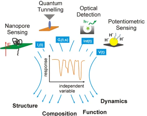
ingle-molecule sensing, sequencing and characterisation based on electric or opticaltechniques can generate very large datasets, in some cases in a (semi-) automated
fashion1-4. This data is typically one-dimensional, in the sense that the conductance,
intensity or current is being recorded as a function of a single, independent variable,
for example time or electrode distance, as illustrated in Fig. 1. The analysis can be
very challenging, not only because of the sheer size of the dataset, but also due to
insufficient knowledge about the characteristic signal features and poor
signal-to-noise ratio (S/N). Some hypothesis-driven data exploration and selection is often
required: Led by an expectation that may for example be informed by a physical
model or even intuition, the experimenter inspects the data either manually or
automatically using some statistical criteria. They would aim to extract data
signatures of interest ('signal'), rejecting supposedly uninteresting 'background' or
'noise'. While this approach undoubtedly has its merits, it can lead to important
information content being missed, to the omission of unexpected results and to bias in
the interpretation of the results. Hand selection may also be highly impractical for
[image:3.595.173.427.216.417.2]large datasets.
Figure 1 | Single-molecule methods and illustrations of typical outputs. A common feature in various single-molecule detection and characterisation techniques is that they often produce large amounts of one-dimensional data, potentially with
relatively complex sub-structure. With limited a priori knowledge about the data, exploration and interpretation can be very challenging. Deep Learning can help explore these complexities.
An alternative is 'all-data point' analysis, where the complete dataset is analysed
without data selection. The disadvantages with this approach include a potentially
very low S/N, depending on the event frequency, an inherent focus on the most
abundant event type, and an inability to identify and quantify sub-populations in the
data.
Tunnelling current-distance (I(s)) spectroscopy used in single-molecule charge
transport studies is a good example in this context. Here, the tunnelling current is
measured as two electrodes are pulled apart, which may be temporarily bridged by
one or more molecules at a time. The process is automated relatively easily, so tens if
not hundreds of thousands of I(s) traces can be generated relatively quickly. The
formation of a molecular bridge is typically thought to result in a constant current
('plateau'), as long as charge transport through the molecule dominates (as opposed to
'through space' tunnelling)5. Sub-populations in the data may arise from different
numbers of molecules in the junction, different molecular configurations or bonding
patterns between the molecule of interest and the electrode surface(s)6-13. The
dynamic stretching process may also affect the junction and hence the measured
tunnelling conductance. Some of these events may be 'rare' by some standards, but
nevertheless physically meaningful and may be probed by variations in the
experimental parameters (e.g., the temperature).
Unfortunately, the exact manifestation of these effects in the I(s) trace is normally
not a priori known, rendering hypothesis-led data exploration difficult, and they may
be too 'rare' to feature in 'all-data' analyses. In cases where multiple event classes
occur simultaneously with comparable probability, the latter approach can even
produce misleading results14. Thus, neither of the two strategies appears entirely
satisfactory in this regard.
Ideally, one would like to look for common features in the data without making
prior assumptions and be able to quantify those in a coherent manner. Only recently, a
Machine Learning (ML) based technique has been introduced that goes some way
towards this goal, namely Multi Parameter Vector Classification (MPVC)14. MPVC
follows a different philosophy, compared to the approaches described above, in that
each data trace is characterised by a classifier of N parameters and thus forms a point
in N-dimensional vector space. In this space, similar data traces then make up
clusters, which can readily be extracted using suitable clustering algorithms (albeit the
definition of what constitutes a cluster is not always trivial). The physical
interpretation of each cluster typically follows the clustering step, potentially with
support from additional, independent experimental data or theory and simulations.
While the formation of clusters does depend on the choice of classifiers and is thus to
some extent subjective, MPVC does not make any assumptions about the signal shape
as such and does not exclude any data. Very recent work by Wu et al. considers this
aspect further by employing hierarchical and density-based clustering in analysing
single-molecule charge transport, which indeed gave very promising results for their
systems15.
Another area where ML techniques have resulted in a notable improvement in
performance is in the field of DNA base detection and sequence analysis. Here, the
challenge is to identify the four DNA bases (and potentially epigenetic and other
DNA modifications) in an a priori unknown sample. While the signal characteristics
of each individual base are typically known and may be used for 'training', the
inherent structure within each event can be quite complex and base differentiation be
fraught by low S/N and context-specific signal variation. To this end, Chang et al. have been able to demonstrate that a Support Vector Machine (SVM) could be used to
enhance tunnelling-based detection of (oligo)nucleotides as well as amino acids16-18.
A SVM is a type of learning model that uses hand-crafted features, e.g., the event
magnitude, duration or other statistical properties, combined in a classifier, to
discriminate between a number of unidentified targets (such as the four DNA
bases).19,20 It is thus the job of the algorithm designer to identify and implement those
features, in the hope of minimising the prediction error as much as possible.
However, even with the training data at hand, it is not at all obvious, which signal
characteristics to choose for the most reliable and most accurate predictions. It would
be advantageous to extract those characteristics from the available data itself, to arrive
at the best possible result.
Interestingly, as a result of recent and dramatic progress in ML so-called "Deep
Learning" (DL) methodologies may be able to do just that21-25. Once the architecture
of a DL network has been designed, in terms of the number of layers that are meant to
characterise the data, typically at different levels of abstraction (or 'resolution'), the
'content' of these layers is then 'learned' from the training data.
In numerous applications, DL has been shown to outperform earlier ML methods,
including SVM, and in some cases such as image and speech recognition, and
complex control tasks, it has even achieved results that surpass human performance
26-28
. In the specific case of DNA or peptide sequencing-by-tunnelling, this raises an
interesting prospect: If the application of an SVM resulted in a significant, albeit from
a technological point of view still insufficient improvement in detection performance,
could DL enable such an important step? More generally in single-molecule sensing,
sequencing, and characterisation, could DL help to identify features in a signal that
were previously unknown or unexpected, but are nevertheless physically meaningful?
In many ways, it could be a step change in the way data is explored, analysed and
interpreted. But a comprehensive understanding of these methods in this new context
is crucial to reaping the benefits and to avoiding the pitfalls - especially, since the link
between data analysis and interpretation on the one hand, and the experimenter's input
and intuition on the other is somewhat weakened. Hence, in this Perspectives article,
we aim to provide an insight into the 'internal workings' of a Convolutional Neural
Network (CNN), as a powerful DL tool for data classification and analysis. We start
with a brief introduction to the field, in order to introduce the terminology and to
explain the basic concepts. As a specific example, we then illustrate the use of a CNN
for simulated, but realistic sets of tunnelling data, and compare its performance with
SVM, as a more conventional ML methodology.
Artificial Neural Networks and Convolutional Neural Networks
Supervised ML algorithms 'learn' a function, or model, given a set of training
examples. Each example is in the form of an input and a matching output –for
instance, in speech recognition, a ML algorithm can learn a function that recognizes
text from audio signals after being trained with examples of recordings of spoken
words and their corresponding text29,30.
Artificial Neural Networks (NN) are a type of supervised ML architecture formed
of layers of units or neurons, in which, for each training example, information from an
input layer is processed in a 'hidden' layer and the result compared against the target,
forming the 'error', in the output layer. The goal of the NN is to minimize the error for
all training examples. Once the neural network has been trained, its accuracy is
evaluated against unseen datasets (see Fig. 2 Top and the technical Jargon Buster for a
more detailed exposition of NN workings).
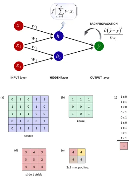
Figure 2 | Top: A schematic representation of a 'shallow' Artificial Neural Network.
A layer of normalized inputs is connected to a hidden layer in which neurons compute the weighted sum of all inputs. A non-linear activation function is applied to the latter, and the result passed on to the output layer. During training, the error is then back-propagated, the weights adjusted using an optimization algorithm and the process repeated until the output matches the target. Bottom:CNN basic steps, convolution and max pooling. (a) represents the source or input data and (b) a 3x3 kernel, filter or feature detector. The kernel is applied to the source by multiplying its values element-wise with the original matrix and summing up the result, (c). This operation is repeated over the source, by sliding (shifting or dilating) the kernel, in this case with 1 stride, which produces the convoluted map (d). Different kernels can be applied to a given input. Another CNN operation that reduces dimensionality is pooling: for example, in (e) we apply max pooling with a 2x2 stride to a source (i.e., in the 2 by 2 submatrix, the maximum value is kept in the pooled result). A CNN typically involves several layers of convolving and pooling layers.
Jargon Buster
A signal is a data trace 'as measured', e.g., as a function of time or distance, including events and event-free segments.
An event is defined as a signal modulation due to some 'molecular' process. An event can have substructure, such as spikes.
A feature is a measurement that characterizes an example (e.g., amplitude or duration of a signal in the context of single molecule sensing). A good feature is discriminative, enabling the machine learning algorithm to make a correct prediction. Deep learning methods learn the features that optimally perform this prediction, unlike methods like SVM that require hand-crafted features.
Activation functions are applied to weighted inputs to produce the NN output. In order to learn complex decision boundaries they must be non-linear (e.g., sigmoid, tanh or ReLU). In two dimensions, the decision boundary can be thought of a line separating two clusters of data points in the best possible way.
The 'vanishing gradient' problem arises in deep NNs that use activation functions whose gradients are small and 'vanish' throughout the layers during backpropagation, preventing the network from learning long-range dependencies. The Rectified Linear Units (ReLU) activation function is a non-linear function defined by f(x) = max(0, x) and used in CNNs to counteract this problem.
The error (aka loss function, cost function or, simply, the objective function) is a measure of the difference between the output and the target or ground truth. The error is fed into abackpropagation algorithm in order to update the weights that process the input in the neural network, in such a way that it generates less error.
Backpropagation is an algorithm that repeatedly applies the chain rule of calculus differentiation for partial derivatives starting from the error in the output layer and propagating the gradients (the ratio of the rate of change of the weights and the error) backwards.
Gradient Descent is an optimization algorithm used to minimize the error by iteratively updating the weight parameters in the direction of the gradient of the loss function. When we randomly select a single data point from our dataset to calculate the gradient, we call it Stochastic Gradient Descent.
Convolutional Neural Networks are deep neural networks, which use convolutions (the integrals measuring how much two functions overlap as one passes over the other) to extract features from local regions of an input. Their depth comes in sequences of convolutional, ReLU, pooling and dropout layers, and final fully-connected layers.
The convolutional layer in a CNN consists of a collection of filters or kernels that convolve (slide) across the input to produce feature maps. The underlying principle is that CNNs use local connectivity and shared weights (the filters) to search for the same features in the input, enforcing invariance and reducing dramatically the number of parameters as compared against traditional fully-connected networks. Importantly, a CNN learns the values of these filters (feature detectors) 'on its own' during the training process.
Pooling is a technique used in CNNs, and consists of sliding a window over patches of features, such as pixels, and taking the average or the maximum of all values within. It compresses (down-sampling) the input representation into a lower-dimensional representation.
Softmax is a function that takes a vector of real values and 'squashes' it to a vector of real values in the range [0, 1] that sum to one (essentially a normalisation procedure). The softmax output can be interpreted as a probability. Softmax is commonly seen as the last stage of a CNN used for classification, and gives a probability that the data being classified is an example of the learned classes.
A second problem that applies to all ML algorithms, is overfitting, which refers to co-adaptation on training data and poor generalization. Within the context of DL and CNNs in particular, dropout is a technique that prevents overfitting by randomly dropping units (along with their connections) from the neural network during training.
Deep networks learn multiple levels of abstractions of data through multiple processing layers. By doing so, the deep network automatically learns the representations (features) that minimize the objective function. In contrast, shallow networks do not learn the features, rather, these are engineered by the algorithm designer.
Neural networks and alternative shallow-structured ML architectures such as SVM
or logistic regression show limited modelling and representational power –
constraining their usefulness to simple, well-constrained problems. Deep neural
networks (aka DL networks) are multi-layer NNs that offer a way to enhance shallow
architectures with the necessary complexity in structure and richness in representation
required to deal with real-life applications. More specifically, in contrast to
conventional ML approaches, DL does not use manually defined, 'hand-crafted'
features. Rather, DL defines hierarchies of layers that 'automatically' learn the data
representation at different levels of abstraction. For instance, in an image recognition
task, the algorithm will be presented with a large noisy set of raw pixels, and learn
first basic low-level features such as curves or shadows, and then categories of
increasing complexity, e.g., nose, ear, elbow, then face, arm, leg, and finally the
concept 'MAN'.
Since, inspired by McCulloch-Pitts neuron model31 and Donald Webb’s work on
synaptic learning32, NNs were first proposed33,34, a number of advancements in
computational power and increasingly sophisticated learning algorithms (ReLU
functions35,36, dropout techniques37) as well as in the availability of large datasets,
have made DL very popular. Crucially, the drawbacks identified in Minsky and
Papert’s seminal paper38, namely that NNs were unable to learn complex non-linear
models, were overcome with the invention of the backpropagation algorithm39,40 and
Hornik’s proof that NNs are universal approximators41, leading to the development of
DL technology in the form of Convolutional Neural Networks42,43, autoencoders44,
Deep Belief Networks45-47 and Recurrent Neural Networks48 (see Fig. 3 for a
historical perspective). The main principle remained the same as in traditional NN
algorithms nonetheless: Outputs are compared against the target, that is, against the
expected outcome. The error is then propagated back to the neurons in previous layers
using a variation of the backpropagation algorithm and minimised by adjusting the
weights of the neurons49.
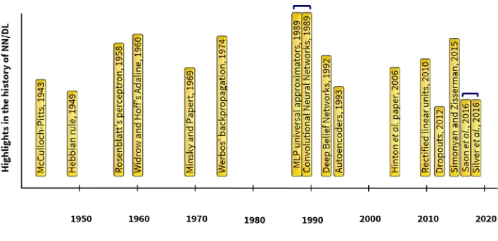
Figure 3 | Timeline of the history of Artificial Neural Networks and Deep Learning.
Deep Learning’s peak corresponds with Hinton’s et al. breakthrough paper50 and the
increase in data size (number of examples) from 105 of MNIST handwritten dataset
at the turn of the twenty-first century to 109 in, for example, the WMT 2014 English
to French dataset51. Likewise, the number of neurons in DL networks has move from
100 in Rosenblatt’s Perceptron to 107 in GoogLeNet52; and in the number of
connections from 101 in ADALINE to104 in COTS HPC unsupervised convolutional
network53. Finally, during the last indiction GPUs have increased computational
power to 104 GFLOPS.
In particular, Convolutional Neural Networks (CNN) learn to extract relevant
information for the recognition of signals in a similar way that an infant has to learn
to group elements in their visual scene in order to make sense of their visual input54.
CNNs are biologically inspired multi-layer networks of convolutional and
subsampling layers, which include constraints in the form of feature extraction
(receptive fields that filter local features), feature mapping (weight sharing, which
forces invariance), and subsampling (pooling or local averaging). The idea is to
translate many low-level features (raw input) into compressed high-level
representations by exploiting local correlation and enforcing local connectivity
patterns between neurons of adjacent layers. In so doing, the CNN can detect
hierarchies of features and complex patterns (see Jargon Buster box). Fig. 2 Bottom
illustrates the basic steps in a CNN with a simple example taken from the analysis
two-dimensional data (such as image classification).
Simulated 'sequencing-by-tunnelling' data
But how can DL be applied to one-dimensional datasets, such as current-time,
intensity-time or current-distance data? In order to explore this further, we produced
simulated 'sequencing-by-tunnelling' data using a simulator developed in Matlab
2016b (Mathworks, Natick MA, script available on request). The simulator is
inspired by experimental results, where binding of DNA bases in an STM junction
was found to modulate the measured tunnelling conductance16. The occurrence of
these binding events, their duration and the observed tunnelling conductance are
stochastic in nature, and dependent on the identity of the molecule. The simulator
takes this into account via the following parameters:
• The signal length, L, representing the total number of data points in each trace
(here: 10,000)
• The number of events E in each signal of length L (a measure for the event
frequency)
• A Normal distribution modelling the event duration, 𝑁(𝑚𝑑,𝜎𝑑), where 𝑚 is
the mean and 𝜎the standard deviation
• A Normal distribution modelling the event height modulation (magnitude of
the current modulation) 𝑁(𝑚𝑚,𝜎𝑚)
• A Normal distribution modelling the noise, 𝑁(𝑚𝑛,𝜎𝑛)
• A switching probability, representing the likelihood of an event having data points with zero conductance, 𝑝𝑠(telegraphic noise)
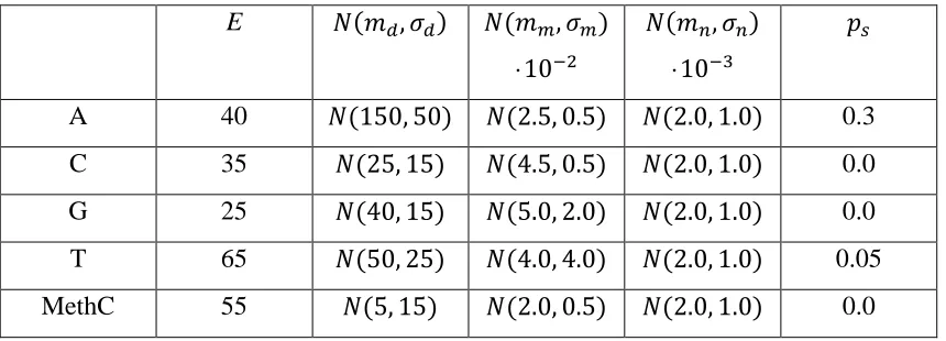
With the simulator, 10,000 signals (i.e. individual traces, with 10,000 data points
each) for the five biomolecules representing DNA bases (A, C, G, T) and
5-methyl-cytosine (MethC) were generated (2,000 traces/biomolecule), with the specific
simulation parameters shown in Table 1.
E 𝑁(𝑚𝑑,𝜎𝑑) 𝑁(𝑚𝑚,𝜎𝑚)
·10−2
𝑁(𝑚𝑛,𝜎𝑛)
·10−3
𝑝𝑠
A 40 𝑁(150, 50) 𝑁(2.5, 0.5) 𝑁(2.0, 1.0) 0.3
C 35 𝑁(25, 15) 𝑁(4.5, 0.5) 𝑁(2.0, 1.0) 0.0
G 25 𝑁(40, 15) 𝑁(5.0, 2.0) 𝑁(2.0, 1.0) 0.0
T 65 𝑁(50, 25) 𝑁(4.0, 4.0) 𝑁(2.0, 1.0) 0.05
[image:12.595.85.515.91.246.2]MethC 55 𝑁(5, 15) 𝑁(2.0, 0.5) 𝑁(2.0, 1.0) 0.0
Table 1 | Parameters used in the simulator to generate biomolecule conductance signals.
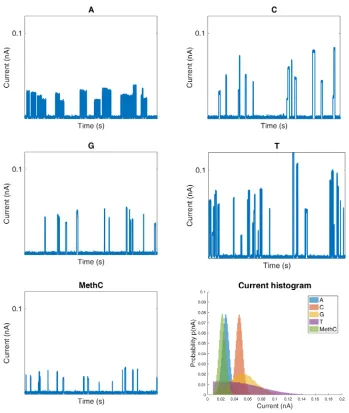
An example trace with several individual events for each of these five classes is
shown in Fig. 4. As shown below, the CNN operates on entire traces, not individual
events. Hence, initial event recognition and extraction is not required. However, the
complexity of the event characteristics, and the significant overlap in their statistical
properties, renders molecular identification from a trace an interesting pattern
recognition problem.
Figure 4 | Example current-time traces produced by the simulator for the five biomolecules. Signals (or traces) consist of events which may have multiple spikes due to a finite switching probability ps (perhaps due to bond formation and breaking).
Event current histograms (bottom right) show that there is considerable overlap between data distributions, which would render differentiation between the molecules very difficult and resulting in a large error rate
Analysis of the simulated data by a CNN
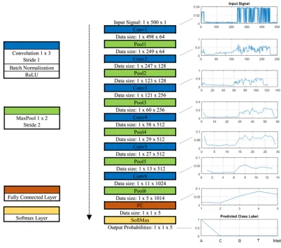
A deep convolutional neural network was thus designed to classify the simulated data
produced. As these are one-dimensional time-domain signals, the network employs a
series of one-dimensional convolutional and pooling layers, as illustrated in the
network diagram in Fig. 5.
In order to keep the computational cost low, we simplified each trace by
identifying the maximum current value, centred this current value within a window of
500 data points. This is shown as the initial 'input signal' in Fig. 5 (top right). In
principle, the network could also process the entire trace of 10,000 data points, which
increases the complexity of the computational task.
There are six convolutional layers, arranged hierarchically so that the later layers
learn a higher level representation of the signal. Each convolutional layer is followed
by a batch normalization layer, a rectified linear unit (ReLU) layer and a max pooling
layer that subsamples the data to produce a lower dimensional representation (a CNN
network typically includes a dropout layer, as in the Jargon Buster; in our case, it was
not needed).
In our case, all the convolutional filters are kernels of size 1x3 and applied to the
temporal data. These can be filters are learned by back propagation, and the resulting
filters are varied, and include local averaging with varying weighting factors (e.g. a
conventional gliding average with window size 3 would have constant weighting
factors of 1/3), differential filters and others. The CNN learns these kernels during
training, i.e. by comparing the calculated output with the known outcome from the
training sample. The error in the output is subsequently 'back-propagated' through all
layers of the network, until the best outcome is achieved. During this process, the
individual weighting factors, which may be assigned randomly at the start, are
optimised, for example using a gradient descent method (as used here) or other
techniques. We note that each convolutional layer has more than one filter - e.g., in Fig. 5 'conv1' has 64, 'conv2' 128 and so forth. Each filter acts on the respective input
signal in a specific way - we show one example of the input signal at each
convolutional layer as they evolve through the network (incl. the Fully Connected
layer).
ReLU introduces non-linearity and helps to avoid the 'vanishing gradient' problem,
as described in Jargon Buster box. We then employ pooling layers that halve the
dimension of the input signal using a so -called 'max-pooling' technique with 1x2
window size and stride of 2 (cf. Fig. 2 Bottom). The final pooling layer is followed by
a fully connected layer and a softmax layer. The softmax layer predicts the categorical
probability of the input signal over the class labels that represent the biomolecule
identity.
In total, the network has 2,913,669 parameters, which are updated using a
stochastic gradient descent during training. The training was done for 30 epochs
(rounds of optimisation), using 7,500 detection events in a training set, 500 in a
validation set, and 2,000 held out for independent testing. On this independent test set,
[image:15.595.90.492.240.595.2]the overall accuracy of the CNN classifier was 98.1%.
Figure 5 | Convolutional neural network architecture for classifying the simulated biomolecule conductance signals. A raw signal is input at the top of the figure, and goes through numerous layers of convolution, ReLU, and max pooling. A fully
connected layer is then connected to a softmax, which produces output probabilities for the five classes (A, C, G, T, and MethC). In this way, a raw signal is transformed to a vector of probabilities. For the example above, there is a high probability it is an adenine molecule (A) and it is the highest probability that is selected as the output
class. The example on the right shows how a raw signal is transformed through the network and results in a prediction of a class A. These plots show one of the signals input to each convolutional and the fully connected layer.
Comparison to shallow learning using hand-crafted features
For comparison, a shallow learning method was developed, inspired by Chang et al,
employing a similar classifier 16-18.
For a meaningful comparison, the same 7,500 signals were used to train the SVM
as the CNN described above. Moreover, the same independent 2,000 signals were
used to test the performance. The overall accuracy of the SVM classifier was 91.7%,
which is a strong result and numerically similar in overall performance to 16 (bearing
in mind that we use simulated data, direct comparison of the performances is not
straightforward).
However, the results can be compared to the CNN method described above.
Although further work could be performed to find additional hand-crafted features to
improve the SVM performance, searching for features is a tedious, and not
necessarily an optimal process. In addition, hand-crafting features may induce bias in
the results. In contrast, the CNN learns its features automatically, and therefore is not
susceptible to bias induced by hand-crafted features. The CNN in this experiment
outperforms the SVM by a large margin that is statistically significant based on a
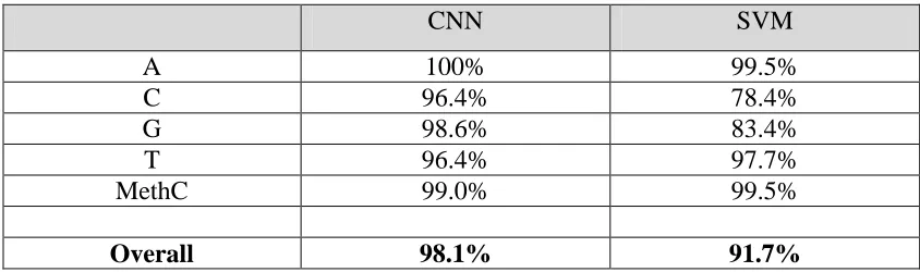
paired t-test at the p<0.05 threshold. Looking at the misclassifications reveals that for
both the CNN and SVM, the A, T, and MethC are classified with low error, however,
[image:16.595.89.511.595.720.2]C and G have a higher number of misclassifications in the SVM model as shown in
Table 2. Overall, the CNN is better at distinguishing these classes.
CNN SVM
A 100% 99.5%
C 96.4% 78.4%
G 98.6% 83.4%
T 96.4% 97.7%
MethC 99.0% 99.5%
Overall 98.1% 91.7%
Table 2 | Classification accuracies for the respective biomolecules for the CNN and SVM methods. The overall accuracy is for an independent test set.
Conclusions
The key question that follows on from these results relates to the broader implications
of the use of DL in single-molecule science, in comparison with more conventional
approaches data analysis, including more advanced methods such as SVMs. Indeed,
the fact that the above CNN performed better on average than the SVM is an
interesting, but singular result. Both could be improved further, for example
increasing the complexity of the network and size of the input data on the one hand,
and by employing a larger number of handcrafted features on the other. That said, a
difference in prediction accuracy of 6.4% can be very significant, especially when
repeat observations lead to an accumulation of errors. For example, for 10 subsequent,
uncorrelated observations, the total accuracy for the CNN is 0.98110 = 0.825 or
82.5%, whereas we obtain 0.91710 =0.420 or 42.0% for the SVM. So the prediction
accuracy is only approximately half that of the CNN.
The need to define hand-crafted features in an SVM has two sides. One the one
hand, this is an opportunity to use features that are informed by some underpinning
physical understanding of the process at hand, for example the magnitude of an event,
its duration or some less obvious event properties characterisation potential
sub-structure. On the other hand, finding good features can be tedious and it is generally
difficult to know beforehand, whether a particular classifier will perform well or
whether it is even close to the best achievable performance. In general, the
experimenter retains a relatively high level of control - or intuitive understanding - of
the analysis process.
The CNN operates in a very different way. While the initial design of the network
includes (human) decisions on the number of layers, the nature of the filters, input
data format etc., the contents of the individual layers after training can be very
difficult to interpret, in terms of some physical meaning. Some attempts in this
direction have been made in image recognition55,56, but at present it is not clear, how
(or whether) a direct physical meaning can be assigned to these layers in the present
context. So from a physical point of view, the CNN is very much a 'black box' - it
may perform very well in a particular task, but it may be difficult to comprehend the
how and why.
An interesting feature of CNNs is that they can operate on entire data traces, as we
have done here, rather than individual events. This avoids the need to produce
potentially subjective 'event-defining' criteria, such as signal thresholds and the like. It
may also be beneficial in cases, where event detection is complicated by strongly
varying backgrounds, such that explicit background correction may no longer be
necessary.
Another aspect of CNNs that should be borne in mind is that a particular
combination of learned weights results from training on a particular training set. If a
CNN were to be retrained with another training set, having been recorded under
nominally the same or perhaps systematically varied conditions (say, at a different
temperature), the new learned weights do not normally extrapolate to the original set.
In this sense, the CNN does not contain any 'knowledge' of the system under study.
'Transfer Learning' is a relatively new branch in Machine Learning, where networks
are trained for a particular task (e.g., a particular computer game) and then confronted
with new one (another computer game)57. This has been shown to work well in some
situations and may be an interesting prospect in the present context.
Finally, could CNNs be used to explore data towards identifying unknown features
in the data? This is not straightforward, but may be possible. For example, if a trained
CNN were to be confronted with an unseen dataset that contain features that were not
present in the training data, then the prediction accuracy would be correspondingly
lower. One approach could then be to extract events, for which the CNN performs
relatively poorly and then try to rationalize the origin of these deviations.
In conclusion, it appears that DL methods and CNNs in particular may have very
interesting and obvious prospects in some areas of single-molecule science, such as
single-molecule detection and sequencing. DL is still a rather new area in Machine
Learning, with major breakthroughs since 2012. It is therefore likely that DL and
other, state-of-the-art Machine Learning techniques will find their way into the
physical sciences and into engineering. Equally, the ability to provide large amounts
of data from rather well-defined experiments, the latter may also help to develop a
better understanding of the internal workings of rather complex networks.
References
1. Levene, M. J. Zero-Mode Waveguides for Single-Molecule Analysis at High
Concentrations. Science 299, 682-686 (2003).
2. Eid, J. et al. Real-Time DNA Sequencing from Single Polymerase Molecules.
Science 323, 133-138 (2009).
3. Gu, L. et al. Multiplex single-molecule interaction profiling of
DNA-barcoded proteins, Nature 515, 554-557 (2014).
4. Bell, N. A. W. & Keyser, U. F. Digitally encoded DNA nanostructures for
multiplexed, single-molecule protein sensing with nanopores. Nat. Nanotechnol. 11, 645-651 (2016).
5. Quan, R., Pitler, C. S., Ratner, M. A. & Reuter, M.G. Quantitative
Interpretations of Break Junction Conductance Histograms in Molecular
Electron Transport. ACS Nano 9, 7704-7713 (2015).
6. Albrecht, T., Mertens, S. F. L. & Ulstrup, J. Intrinsic multistate switching of
gold clusters through electrochemical gating. J. Am. Chem. Soc. 129,
9162-9167 (2007).
7. Inkpen, M. S. et al. New insights into single-molecule junctions using a robust, unsupervised approach to data collection and analysis. J. Am. Chem.
Soc. 137, 9971-9981 (2015).
8. Albrecht, T. Electrochemical tunnelling sensors and their potential
applications. Nat. Commun. 3, 829 (2012).
9. Yoshida, K. et al. Correlation of breaking forces, conductances and
geometries of molecular junctions. Sci. Rep. 5, 9002 (2015).
10.Kihira, Y., Shimada, T., Matsuo, Y., Nakamura, E. & Hasegawa, T. Random
telegraphic conductance fluctuation at Au-pentacene-Au nanojunctions. Nano
Lett. 9, 1442-1446 (2009).
11.Adak, O. et al. Flicker noise as a probe of electronic interaction at
metal-single molecule interfaces. Nano Lett. 15, 4143-4149 (2015).
12.Su, T. A., Li, H., Steigerwald, M. L., Venkataraman, L. & Nuckolls, C.
Stereoelectronic switching in single-molecule junctions. Nat. Chem. 7,
215-220 (2015).
13.Fujihira, M., Suzuki, M., Fujii, S. & Nishikawa, A. Currents through single
molecular junction of Au/hexanedithiolate/Au measured by repeated
formation of break junction in STM under UHV: effects of conformational
change in an alkylene chain from gauche to trans and binding sites of thiolates
on gold. Phys. Chem. Chem. Phys. 8, 3876-3884 (2006).
14.Lemmer, M., Inkpen, M.S., Kornysheva, K., Long, N.J. & Albrecht, T.
Unsupervised vector-based classification of single-molecule charge transport
data. Nat. Commun. 7, 12922 (2016).
15.Wu, B. H., Ivie, J. A., Johnson, T. K. & Monti, O.L.A. Uncovering
hierarchical data structure in single molecule transport. J. Chem. Phys. 146, 092321 (2017).
16.Chang, S. et al. Chemical recognition and binding kinetics in a functionalized
tunnel junction. Nanotechnology 23, 235101(2012).
17.Chang, S. et al. Palladium electrodes for molecular tunnel junctions.
Nanotechnology 23, 425202 (2012).
18. Zhao, Y. A. et al. Single-molecule spectroscopy of amino acids and peptides
by recognition tunnelling. Nat. Nanotechnol. 9, 466-473 (2014).
19.Cortes, C. & Vapnik, V. Support-Vector Networks. Machine Learning 20,
273-297 (1995).
20.Dietterich, T. G. & Bakiri, G. Solving Multiclass Learning Problems via
Error-Correcting Output Codes. J. Artif. Intell. Res. 2, 263-286 (1994).
21.Bengio, Y. Deep Learning Architectures for AI. Foundations and Trends in Machine Learning 2, 1-127 (2009).
22.Deng, L. & Yu, L. D. Deep Learning: Methods and Applications. Foundations
and Trends in Signal Processing 7, 1–199 (2013).
23.LeCun, Y., Bengio, Y. & Hinton, G. Deep Learning, Nature 521, 436–444
(2015).
24.Goodfellow, I., Bengio, Y. & Courville, A. Deep Learning (The MIT Press, Cambridge, MA, 2016).
25.Schmidhuber, J. Deep Learning in Neural Networks: An Overview. Neural Netw. 61, 85-117 (2015).
26.Simonyan, K. & Zisserman, A. Very Deep Convolutional Networks for
Large-Scale Image Recognition. ICLR 2015 (arXiv:1409.1556) (2015).
27.Saon, G., Sercu, T., Rennie, S. & Kuo, H-K. J. The IBM 2016 English
Conversational Telephone Speech Recognition System. InterSpeech 2016 (arXiv:1604.08242v1) (2016).
28.Silver, D. et al. Mastering the Game of Go with Deep Neural Networks and
Tree Search. Nature 529, 484-489 (2016).
29.Mitchell, T. Machine Learning (McGraw-Hill, New York City, NY, 1997).
30.Bishop, C. M. Pattern Recognition and Machine Learning (Springer, New York City, NY, 2006).
31.McCulloch, W. S. & Pitts, W. A logical calculus of the ideas immanent in
nervous activity. Bull. Math. Biophys. 5, 115–133 (1943).
32.Hebb, D.O. The organization of behavior: A neuropsychological theory (John
Wiley & Sons, Hoboken, NJ, 1949).
33.Rosenblatt, F. The Perceptron: A Probabilistic Model for Information Storage
and Organization in the Brain. Psychol. Rev. 65, 386–408 (1958).
34.Widrow, B. An Adaptive “Adaline” neuron using chemical ”memistors”.
Number Technical Report 1553-2 (Stanford Electron. Labs, Stanford, CA,
1960).
35.Nair, V. & Hinton, G. E. Rectified linear units improve restricted Boltzmann
machines. ICML, 807-814 (2010).
36.Glorot, X., Bordes, A. & Bengio, Y. Deep sparse rectifier neural networks.
ICAIS, 315-323 (2011).
37.Hinton, G. E., Srivastava, N., Krizhevsky, A., Sutskever, I. & Salakhutdinov,
R.R. Improving neural networks by preventing co-adaptation of feature
detectors (arXiv:1207.0580) (2012).
38.Minsky, M. & Papert, S. A. Perceptrons: An Introduction to Computational
Geometry (The MIT Press, Cambridge, MA, 1969).
39.Werbos, P. Beyond Regression: New Tools for Prediction and Analysis in the
Behavioral Sciences (Harvard University, Cambridge, MA, 1974).
40.Rumelhart, D. E., Hinton, G. E. & Williams, R. J. Learning representations by
back-propagating errors. Nature 323, 533-536 (1986).
41.Hornik, K., Stinchcombe, M. &White, H. Multilayer feedforward networks
are universal approximators. Neural Netw. 2, 359-366 (1989).
42.LeCun, Y. et al. Backpropagation Applied to Handwritten Zip Code
Recognition, Neural Comput. 1, pp.541-551 (1989).
43.LeCun, Y. et al. Comparison of learning algorithms for handwritten digit
recognition. ICANN, 53-60 (1995).
44.Hinton, G. E. & Zemel, R. S. Autoencoders, Minimum Description Length
and Helmholtz Free Energy. NIPS, 3-10 (1993).
45.Neal, R. M. Connectionist learning of belief networks. Artificial intelligence 56, 71-113 (1992).
46.Hinton, G. E., Dayan, P., Frey, B. J. & Neal, R. M. The wake-sleep algorithm
for unsupervised neural networks. Science 268, 1158-1161 (1995).
47.Dayan, P., Hinton, G. E. & Neal, R. M. The Helmholtz Machine. Neural Comput. 7, 889-904 (1995).
48.Goller, C. & Küchler, A. Learning task-dependent distributed representations
by backpropagation through structure. IEEE Trans. Neural Networks, 347-352
(1996).
49.Bengio, Y., Lamblin, P., Popovici, D. & Larochelle, H. Greedy layer-wise
training of deep networks. NIPS 19, 153-160 (2007).
50.Hinton, G. E., Osindero, S. & Teh, Y-W. A fast learning algorithm for deep
belief nets. Neural Comput. 18, 1527-1554 (2006).
51.Schwenk, H. Cleaned subset of WMT’14 dataset.
http://www.statmt.org/wmt14/translation-task.html (2014).
52.Szegedy, C. et al. Going deeper with convolutions (arXiv:1409.4842) (2014).
53.Coates, A. et al. Deep learning with COTS HPC systems. ICML 28, 1337-1345 (2013).
54.LeCun, Y., Bottou, L., Bengio, Y. & Haffner, P. Gradient-Based Learning
Applied to Document Recognition. Proc. IEEE 86, 2278–2324 (1998).
55.Simonyan, K., Vedaldi, A. & Zisserman, A. Deep Inside Convolutional
Networks: Visualising Image Classification Models and Saliency Maps. ICLR
(arXiv:1312.6034) (2014).
56.Zeiler, M. D., & Fergus R. Visualizing and Understanding Convolutional
Networks. ECCV, 818-833 (2014).
57.Yosinski, J., Clune, J., Bengio, Y. & Lipson, H. How Transferable are
Features in Deep Neural Networks? NIPS, 3320-3328 (2014).
Acknowledgements
We thank E. Mondragón for help with figures.
Author contributions
T.A., and E.A. established the background of the manuscript. G.S. and S.M.M.R.A.A.
performed the experiments. T.A., E.A. and G.S. analysed the data, discussed the
results and wrote the paper.
Additional information
The authors declare no competing financial interests. Supplementary information
accompanies this paper at Data availability and Code availability above.
Correspondence and requests for material should be addressed to T.A.
Deep Learning Resources Software
• Theano, http://deeplearning.net/software/theano/, an open source deep learning
library for Python.
• PyLearn2, http://deeplearning.net/software/pylearn2/ an open source deep learning
library for Python built on top of Theano.
• Torch, http://torch.ch an open source deep learning library and scripting language for
Lua.
• Caffe, http://caffe.berkeleyvision.org, an open source deep learning library for Python
and Matlab.
• MXNet, http://mxnet.io an open source deep learning library for Python, Scala, R,
Julia, and C++.
• TensorFlow, https://www.tensorflow.org, an open source deep learning library for
Python and C++ developed by Google.
• DeeplearningforJ, https://deeplearning4j.org, an open source deep learning library
written for Java and Scala.
• MatConvNet, http://www.vlfeat.org/matconvnet/, a Matlab library for Convolutional Neural Networks.
Datasets
• MNIST, database of handwritten digits, available from this page, has a training set of
60,000 examples, and a test set of 10,000 examples.
http://yann.lecun.com/exdb/mnist/
• ImageNet, a large image database for visual recognition research according to the
WordNet hierarchy (a large lexical database of English), in which each node of the
hierarchy is depicted by hundreds and thousands of images. Currently we have an
average of over five hundred images per node. The ImageNet project runs the Large
Scale Visual Recognition Challenge (ILSVRC).
http://www.image-net.org/
• The CIFAR-10 dataset consists of 60000 32x32 colour images in 10 classes, with
6000 images per class. There are 50000 training images and 10000 test images.
https://www.cs.toronto.edu/~kriz/cifar.html
• Sports-1M is a database containing 1,133,158 video URLs which have been
annotated automatically with 487 Sports labels using the YouTube Topics API.
https://github.com/gtoderici/sports-1m-dataset/
• UC Irvine Machine Learning Repository, general repository with 360 data sets,
including the popular Iris.
http://archive.ics.uci.edu/ml/