Artificial-Intelligence Method for the Derivation of
Generic Aggregated Dynamic Equivalent Models
Eleftherios O. Kontis,
Student Member, IEEE,
Theofilos A. Papadopoulos,
Senior Member, IEEE,
Mazheruddin H. Syed,
Member, IEEE,
Efren Guillo-Sansano,
Student Member, IEEE,
Graeme M. Burt,
Member, IEEE,
and Grigoris K. Papagiannis,
Senior Member, IEEE
Abstract—Aggregated equivalent models for the dynamic anal-ysis of active distribution networks (ADNs) can be efficiently developed using dynamic responses recorded through field mea-surements. However, equivalent model parameters are highly affected from the time-varying composition of power system loads and the stochastic behavior of distributed generators. Thus, equivalent models, developed through in-situ measurements, are valid only for the operating conditions from which they have been derived. To overcome this issue, in this paper, a new method is proposed for the derivation of generic aggregated dynamic equivalent models, i.e., for equivalent models which can be used for the dynamic analysis of a wide range of network conditions. The method incorporates clustering and artificial neural network techniques to derive robust sets of parameters for a variable-order dynamic equivalent model. The effectiveness of the proposed method is evaluated using measurements recorded on a laboratory-scale ADN, while its performance is compared with a conventional technique. The corresponding results reveal the applicability of the proposed approach for the analysis and simulation of a wide range of distinct network conditions.
Index Terms—Artificial Neural Networks, black-box modeling, clustering, dynamic modeling, measurement-based approach.
I. INTRODUCTION
T
HE advent of microgrids (MGs) and the increased pen-etration of distributed generators (DGs) into the existing distribution grids have changed drastically the dynamic prop-erties of power systems [1]–[3]. Under these new operating conditions, academia and power system operators have initi-ated serious efforts to develop accurate and adaptive dynamic simulation models to enhance the analysis of modern active distribution networks (ADNs) [3] as well as to investigate more efficient modes of operation for the DGs.Manuscript received June, 2018, revised October and December, 2018. E. O. Kontis and G. K. Papagiannis are with the Power Systems Laboratory, School of Electrical and Computer Engineering, Aristotle University of Thessaloniki, Thessaloniki, Greece, GR 54124, (e-mail: [email protected]; [email protected]).
T. A. Papadopoulos is with the Power Systems Laboratory, Department of Electrical and Computer Engineering, Democritus University of Thrace, Xanthi, Greece, GR 67100, (e-mail: [email protected]).
M. H. Syed, E. Guillo-Sansano, and G. M. Burt are with the Insti-tute for Energy and Environment, University of Strathclyde, Glasgow, UK, (e-mail: [email protected]; [email protected]; [email protected]).
The work of E. O. Kontis was conducted in the framework of the act ”Support of PhD Researchers” under the Operational Program ”Human Resources Development, Education and Lifelong Learning 2014-2020”, which is implemented by the State Scholarships Foundation and co-financed by the European Social Fund and the Hellenic Republic.
The work in this paper has been supported by the European Commission, under the FP7 project ELECTRA (grant no: 609687) and under H2020 project ERIGRID (grant no:654113).
In the literature, there are several publications using detailed models to investigate the dynamic properties of ADNs and MGs [4]–[6]. However, the development of detailed dynamic models requires very accurate information concerning the structure of the examined grid and the control parameters of the installed DGs. Therefore, this approach requires accurate data, which cannot be determined in distribution networks due to their extended size. Additionally, it is worth noticing that this approach requires significant computational resources, leading also to large simulation times [1].
To reduce the computational burden of dynamic simulations, reduced order dynamic equivalent models have been proposed. The work on this field can be classified into three main ap-proaches [7]. The first one contains coherency-based methods, where group of coherent generators are identified and replaced by equivalent generators. In the second methodology approxi-mate linear models of the examined system are derived using modal analysis techniques. However, in both approaches, the identification of model parameters requires detailed network information, thus the drawbacks and restrictions of detailed modeling apply to these methods as well [8].
techniques, model parameters that are valid only for a narrow range of network conditions can be estimated [1], [9].
To develop generic equivalent models, able to account for a wide range of network conditions, the use of artificial-intelligence techniques have been proposed in the literature.In [16] and [17], dynamic equivalent models based on recurrent artificial neural networks (ANNs) and radial basis functions ANNs are proposed. However, the parameters of these models have no physical meaning [18], thereby offering limited insight to power system engineers concerning dynamic properties of the grid. To address this issue, in [12], [19], [20] artificial intelligence techniques are proposed to derive generic param-eters for conventional equivalent models. More specifically, in [19] support vector clustering is proposed to derive generic pa-rameters for a transfer function-based equivalent model, while in [12] and [20] the use of ANNs is proposed to generalize the parameters of power system load models.However, these methods present certain shortcomings and limitations. For instance, the method proposed in [19] requires measurements from all ADN feeders to provide consistent results, while the approaches of [12] and [20] are focused on conventional load models [21], which cannot describe effectively the dynamic behavior of modern ADNs [1], [22], [23]. Moreover, the performance of the above approaches has only been tested using simulation results. Thus, their applicability for real field applications still remains an open issue.
Considering the above issues, the primary scope of the paper is to develop a new method for the derivation of generic measurement-based equivalent models, suitable for the dynamic analysis of modern ADNs and for the simulation of a wide range of distinct network conditions. The second objective is to evaluate the performance of the proposed method using laboratory measurements.
The proposed method receives as inputs the operating condi-tions (i.e. voltage level, real and reactive power consumption or production), the load and the generation mix of the examined ADN. Using these inputs, an aggregated ADN model is automatically developed, describing efficiently the dynamic behavior of the examined ADN. To fulfill this objective, clustering and ANN techniques are used to derive robust sets of parameters for the variable-order aggregated equivalent model of [22]. This model structure is selected as it allows the simulation of bi-directional power flow phenomena which may occur in modern ADNs during voltage events [22] as well as the simulation of complex power system dynamics, occurring after small or large system disturbances [14].Additionally, the parameters of this model have a strong physical meaning [14]. The effectiveness of the proposed method is evaluated under various network configurations, load and generation mixes, operating conditions and voltage disturbances, using measure-ments acquired from a laboratory-scale ADN. Additionally, its performance is compared with a conventional approach, in which robust sets of parameters are determined based on mean characteristics, by applying statistical analysis.
II. DYNAMICEQUIVALENTMODEL
[image:2.612.319.564.163.338.2]The dynamic response of a distribution network subjected to a step-down voltage disturbance (Fig. 1a) is presented in
Fig. 1b. As shown, immediately after the disturbance, the power demand decreases instantaneously to y+ value. After this transient undershoot a recovery phase occurs and the power gradually recovers to the new steady-state value, i.e.
yss. This dynamic behavior can be accurately simulated using
the aggregated equivalent model of [22]. The block diagram representation of this model is depicted in Fig. 2, while its mathematical formulation is given in the following equations:
yd(t) =yt(t) +yr(t) (1)
where
yr(t) =L−1[g2(s)G(s)] (2)
yt(t) =y0
λ1 V
L(t) V0
+λ2
,
2 X
i=1
λi= 1 (3)
ys(t) =y0
κ1 V
L(t) V0
+κ2
,
2 X
i=1
κi = 1 (4)
g1(t)≡yt(t), g2(t)≡ys(t)−yt(t) (5)
G(s) = n
X
i=1
ci s−pi
(6)
Here, yd(t) can represent both real and reactive power
responses. Functions yt(t) and ys(t) are two polynomial
functions, used to simulate the transient and the steady-state response of the examined ADN [22], [23], respectively. Moreover,λ1,λ2 and κ1,κ2 are the polynomial coefficients of yt andys, respectively [22], [23]. The recovery response
of the power, i.e.yr(t), is approximated using functionsg2(s) andG(s) [14], [22]. g2(s) denotes the Laplace transform of
g2(t), while G(s) is a variable-order linear transfer function [14], [22].p andcstand for the poles and residues ofG(s), respectively, whilen denotes the optimal order of G(s). The optimal orderncan be determined automatically by applying the iterative procedure proposed in [22]. Finally,VL(t)is the
ADN voltage, whereas y0 andV0 are the power and voltage magnitude prior to the examined disturbance.
Time
Voltage Magnitude
Time
Power Demand
y
+
t0 t0
y
0
V
0
V
+ V
ss
a) b)
y
ss
A ( y
ss ,Vss )
B ( y
+ ,V+ )
Fig. 1. a) Indicative step-down voltage disturbance. b) Representative real or reactive power response.
VL
g2(s) G (s)
g1(t)
yd(t) L-1[g
2 (s) G(s)]=yr (t)
Σ
g1 (t)≡yt (t) [image:2.612.314.563.549.633.2] [image:2.612.319.560.667.723.2]III. PROPOSEDGENERICMODELINGAPPROACH
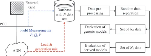
The procedure used to develop the proposed modeling approach is conceptually summarized in Fig. 3. Initially, a database is developed, containing N data sets. In each data set, the following variables are stored: three vectors containing the measured dynamic responses (i.e. RMS values of time-domain signals) of i) voltage (Vi), ii) real (Pi) and iii) reactive
power (Qi). These responses reflect the dynamic behavior of the ADN during the i-th disturbance (i = 1, ..., N) and can be recorded at the point of common coupling (PCC) with the external grid using phasor measurement units (PMUs) [1], [2]. Moreover, two additional variables, namely the iv) load (LMi)
and v) generation mix (GMi) are used. These variables reflect
the load composition and the type of the installed DG units, respectively. The values of LMi and GMi can be assessed
through forecasts or smart meter recordings [24]–[26]. Once the database has been developed, a pre-processing phase is applied. During this phase, the pre-disturbance steady-state values of voltage (V0,i), real (P0,i), and reactive power
(Q0,i) are derived for all the available N data sets. This
information is used to provide an insight of the ADN operating conditions prior to the examined disturbance. Additionally, all dynamic responses are normalized, using the corresponding pre-disturbance steady-state values. Afterwards, the available
N data sets are randomly split into two separate groups, consisting of ND and NT data sets, respectively. The first
group is used to develop generic equivalent models, suitable for the analysis of a wide range of network conditions, while the remaining NT data are used to test the performance of
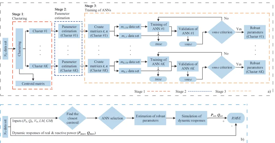
the derived models. The procedures, to develop and test the derived models, are depicted in Figs. 4a and 4b, respectively. As shown in Fig. 4a, the proposed method consists of three main stages: i) clustering of available data, ii) parameter estimation, and iii) training of ANNs. The objective of the clustering is to automatically (i.e. without human interaction) divide the available data into K groups, presenting similar pre-disturbance operating conditions. Then, for each cluster, a multi-signal identification procedure is performed to estimate the model parameters that optimally simulate the dynamic behavior of the ADN. Finally, for each cluster, an ANN is developed. Scope of the ANN is to capture general relation-ships between the model parameters and the examined network conditions. Using this information, robust sets of parameters are derived. A detailed explanation is presented below.
A. Stage 1: k-means++ Clustering Algorithm
At this stage, clustering is applied to automatically divide the available data intoK groups, that present similar charac-teristics. The clustering algorithm, used in this paper, is the
k-means++, an algorithm of proved efficiency for a wide range of applications [27], [28].
In the proposed framework, voltage magnitude, real and reactive power flows at the PCC are monitored by distribution system operator (DSO), using PMU devices [29]. On the other hand, load and generation mix (i.e. variables LM andGM) of the ADN are estimated by the DSO based on forecasts or smart meter recordings. Therefore, in case of forecasts errors,
ADN External
Grid
PCC
Field Measurements P, Q, V
Database with N data
sets
Load & generation mix
Data pre-processing
Random data seperation
Set of ND data
Derivation of generic models
Set of NT data
[image:3.612.316.557.58.148.2]Evaluation of derived models
Fig. 3. Conceptual description of the proposed method.
errors in the values of these variables may be observed. Thus, to reduce the impact of forecast errors in the accuracy of the proposed method, variablesLM andGM are neglected from the clustering procedure. Hence, the clustering is performed based only on the pre-disturbance operating conditions of the ADN, i.e. based onV0,j,P0,j, andQ0,j (herej= 1, ..., ND).
To apply the clustering, V0,j, P0,j, and Q0,j are combined,
for each of the availableND data sets, into one single vector Xj = [V0,j, P0,j, Q0,j]. Thus, a set X of ND observations
X = {X1,X2, ...,XN D} is formed (where each
observa-tion is a d dimensional vector) and forwarded as input to the k-means++ algorithm. Then, the k-means++ algorithm clusters the ND available data sets into K (≤ ND) clusters C={C1, C2, ..., CK}in order to minimize the within cluster
sum of squares [28], as shown in (7).
arg min C
K
X
k=1 X
Xj∈C
||Xj−µk||2 (7)
Whereµk is the mean value of the points in thek-th cluster.
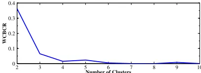
Each cluster of data is represented by its centroid, which defines a representative location in the d dimensional space for all the members of that particular cluster. To derive the optimal number (i.e. K) of clusters, the knee-point criterion for the curve of the Within Cluster sum of squares to Between Cluster sum variation Ratio (WCBCR) is used [30]. According to this criterion, the optimal number of clusters is defined by the knee of the curve [30].
B. Stage 2: Parameter Estimation
At this stage, the dynamic responses of voltage, real and reactive power, i.e. vectors Vj, Pj and Qj, are used to
estimate the model parameters, i.e.θj= [κ1, κ2, λ1, λ2,p,c]. Assuming a set of m data sets for the k-th cluster, the following multi-signal analysis is performed:
Step 1:For each one of themdata sets, parametersκ1,κ2,
λ1, and λ2 are identified from operating points (please refer to Fig. 1)A (yss,Vss) andB (y+,V+), respectively, using the
following equations [22]:
κ1= [V0(yss−y0)]/[y0(Vss−V0)], κ2= 1−κ1 (8)
λ1= [V0(y+−y0)]/[y0(V+−V0)], λ2= 1−λ1 (9)
here, V+ andVss are voltage magnitude at PCC immediately
after the disturbance and at the new steady-state, respectively.
Step 2:The polynomial functions g1 andg2 are computed
ND
d
at
a
se
t
C
lu
st
er
in
g
Cluster #1
. . .
Cluster #K
Parameter estimation (Cluster #1)
Centroid matrix
m1,TRdata set
m1,Vdata set
Training of
ΑΝΝ #1 Validation of
ΑΝΝ #1 Create
matrices t, x
(Cluster #1)
Parameter estimation (Cluster #K)
Create matrices t, x
(Cluster #K)
Robust parameters (Cluster #1)
. . .
. . .
. . .
NT
d
at
a
se
t
Find the closest centroid
ANN selection Simulation of RMSE
dynamic responses Inputs (P0, Q0, V0, LM, GM)
Dynamic responses of real & reactive power (Pmeas, Qmeas)
+
-Stage 1: Clustering
Stage 2: Parameter estimation
Stage 3: Training of ANNs
Stage 1 Stage 2 Stage 3 a)
b)
vmse tmse
vmse criterion Yes No
mK,TRdata set
mK,Vdata set
Training of
ΑΝΝ #K Validation of
ΑΝΝ #K
Robust parameters (Cluster #K)
vmse tmse
vmse criterion Yes No
. . .
Estimation of robust parameters
[image:4.612.78.527.65.298.2]Pest, Qest
Fig. 4. Flowchart of the proposed modeling approach. a) Procedure for the derivation of generic dynamic equivalent models and b) procedure used to test the performance of the derived models.
Step 3: Here, (1) and (2) are used and m individual
responses are derived for the G(s).
Step 4: The m distinct responses of G(s) are grouped
together and inserted as inputs to the Vector Fitting (VF) algorithm [14], [31]. Using the VF, the m distinct G(s)
responses are approximated via a common set of poles and
m distinct set of residues.The use of a common set of poles implies that all responses, belong at the same cluster, are approximated using a model of the same order, i.e., the value of parameter n is common for all m responses. Therefore, following this approach, only the dominant system modes are included in the developed model [32]. A detailed analysis of the parameter estimation procedure can be found in [14].
C. Stage 3: Derivation of Robust Parameters using ANNs
Scope of this stage is to generalize the parameters of the equivalent model in order to extend its applicability for the analysis of a wide range of network conditions, i.e. for network conditions different from those it has been originally developed using the available training data.
In this paper, the two-layer feed-forward ANN of Fig. 5 is used for the generalization of the model parameters. The proposed ANN consists of a hidden and an output layer. Each layer contains [33]: an input matrixx, a weight matrixW, a bias matrixb, a sum operator, a transfer functionf, denoted as TF, and the output matrixy. The weighting matrix weights the input elements, while the bias vector biases the corresponding weighted inputs. The sum operator gathers the biases and the weighted inputs and generates an intermediate variable for the associated TF. The TF produces the final outcome of the layer [33]. The input/output relationship in both the output and the hidden layer can be represented as:
y=f(WTx+b) (10)
Hidden Layer
x w
b
f w
b
f y
Output Layer
[image:4.612.319.547.344.407.2]Input Ouput
Fig. 5. Structure of the proposed ANN.
The inputs (x) of the proposed ANN include: the pre-disturbance steady-state values of voltage, real and reactive power at the PCC as well as the load and the generation mix of the examined ADN. The targets (t) are the corresponding equivalent model parameters.xandtcan be written as:
x=
P0,1 ... P0,mk,T R Q0,1 ... Q0,mk,T R V0,1 ... V0,mk,T R
LM1 ... LMmk,T R
GM1 ... GMmk,T R
(11)
t=
κ1,1 ... κ1,mk,T R λ1,1 ... λ1,mk,T R
c1 ... cmk,T R
(12)
where mk,T R denotes the number of data sets that belong
to the k-th cluster and are used for the training of the corresponding ANN. Note that the following set of parameters:
θκ2 = [κ2,1, ..., κ2,mk,T R], θλ2 = [λ2,1, ..., λ2,mk,T R], and p
are not included in the target matrix. The latter is omitted, since all dynamic responses contained in a specific cluster are approximated using a common set of poles. On the other hand, θκ2 andθλ2 can be directly computed from (8)
and (9) using the values of θκ1 = [κ1,1, ..., κ1,mk,T R] and θλ1 = [λ1,1, ..., λ1,mk,T R], respectively. Following this
During the training process, the proposed ANN captures general relationships between the inputs (i.e. conditions of the examined ADN) and the targets (parameters of the equivalent model). Once the training is finished, this information can be used to derive model parameters that simulate adequately new network conditions, i.e. network conditions different from those used for the training of the ANN. To derive the general relationships between network conditions and the model pa-rameters, the ANN iteratively adjusts its weights and biases to minimize the following mean squared error (mse):
mse= 1
R R
X
r=1
t(r)−y(r)2 (13)
R is the total number of elements contained in tandy. An issue that may occur during the training phase is the so-called overfitting problem [33]. In this case, the ANN memorizes the training examples but does not learn to gener-alize to new inputs. Therefore, fails to predict reliably future observations [33]. To improve the generalization capabilities of the proposed ANN and to avoid overfitting issues, in this paper, the early stopping technique is adopted [33]. For this purpose, as shown in Fig. 4a, themdata sets of thek-th cluster are randomly divided into two subsets, containingmk,T Rand mk,V data, respectively. The former is the training set and
it is used to update weights and biases of the ANN. The second one is the validation set. Themseis monitored during the training process for both the training and the validation data sets. The corresponding mse is denoted as tmse and
vmse, respectively. During the initial phase of the training, both the tmse and the vmse decreases. However, when the ANN begins to overfit the training data, the vmse begins to rise. If the validation error increases for a specified number of iterations (six in this paper), the training is terminated and weights and biases are set to the values which correspond to the minimum validation error [33].
Concerning the training of the proposed ANN, a number of critical parameters must be defined [33], [34], i.e. the TF for the hidden and the output layer, the training algorithm and the number of neurons per layer. The TF for the output layer must be the linear (purelin) function to allow outputs to acquire any finite value [33]. On the other hand, the TF for the hidden layer can be either thelog-sigmoid(logsig) or the
tan-sigmoid (tansig) function [33], [34]. Concerning the training
algorithm, a method compatible with the early stopping tech-nique, must be used [33]. Regarding the number of neurons, in the literature there are no specific guidelines for defining the optimum number [12], [33]. Therefore, to optimally define all the above parameters, a parametric analysis is conducted. The corresponding results are presented in Section IV.
D. Testing Procedure
In this phase, the remaining NT data are used to
cross-validate the performance of the derived equivalents. The testing is performed as depicted in Fig. 4b. Initially, the most suitable ANN is selected. For this purpose, testing data are compared with the K centroids using the Euclidean distance
[27]. The selected ANN corresponds to the most similar centroid (i.e. the centroid with the lowest Euclidean distance). Afterwards, variables P0, Q0, V0, LM, and GM of the testing data are forwarded as inputs to the corresponding ANN. Then, the ANN calculates a new set of model parameters for the adopted equivalent model, that describes effectively the corresponding network conditions. This set of parameters is determined based on the general relationships (i.e. the rela-tionships between network conditions and model parameters), which have been derived during the training phase.
Subsequently, the resulting model parameters are used to regenerate the real and reactive power responses of the ADN. To accomplish this, the dynamic responses of voltage are introduced as inputs in the block diagram of Fig. 2. The output of the block diagram contains the estimated real or reactive power responses. The estimated responses are then compared with the actual measurements by means of root mean square errorRM SE, which is defined as:
RM SE=
v u u t
1 T
T
X
τ=1
ymeas(τ)−yest(τ)
2
(14)
where ymeas(τ) and yest(τ) are the measured and the
esti-mated responses at sample τ, respectively, andT is the total number of samples.
E. Online Application of the Proposed Method
A significant advantage of the proposed method is that can be used for online applications, e.g. control room applications. In this case, the following procedure is applied: Initially, the DSO develops the required database. Using this database, the training (i.e. clustering, parameter estimation, training of ANNs) is performed off-line. Once the training is completed, the derived ANNs can be used for online applications.
During the online application, the DSO introduces the oper-ating conditions of the ADN, the load and the generation mix to the corresponding ANN. Subsequently, the ANN provides in close to real-time a set of model parameters, that optimally describe the corresponding network conditions. The DSO can use these equivalents to conduct large-scale simulations to evaluate the dynamic behavior of the ADN under several contingencies and to investigate the interaction of the ADN with the main transmission grid.
IV. EVALUATION OF THEPROPOSEDMETHODUSING
LABORATORYMEASUREMENTS
A. System Under Study
AM1
PVS
P
C
C
S1
5.5 kVA cosφ=0,87
S
ub
-gr
id
#
2
S
ub
-gr
id
#
1
L1
S3
S4
S5
SG
10 kW 7.5 kVAr SLB
AM3 S2 L2
S6
S7
S8
AM2 cosφ=0,877.5 kVA
7.5 kVA cosφ=0,87
DG1 AC
DC 10 kVA
[image:6.612.51.290.59.230.2]2 kVA
Fig. 6. Laboratory-scale ADN.
a dc motor and follows an active power - frequency (P
-f), reactive power - voltage (V-Q) droop control scheme. Sub-grid #2 contains a 10 kVA inverter interfaced distributed generator (DG1), which operates under a constant power (i.e.
P-Q) mode, injecting fixed amount of real power. This unit is used in the experimental setup to emulate the behavior of inverter interfaced DGs [8]. In sub-grid #2 two 7.5 kVA, 0.87 lagging asynchronous machines (AM2 and AM3) are also installed. The torque of all induction machines is controllable. Thus, they can operate both as motors or generators. In the former case, induction machines are used to emulate the dynamic behavior of conventional rotating power system loads [35], while in the latter to imitate the behavior of induction generators [36].
A variety of network configurations is examined by switch-ing on and off the switches of the test setup (S1 - S8). Different loading conditions are examined by altering the power of the installed components. To emulate different oper-ating conditions, the voltage level at the PCC ranges between 360 V (0.9 p.u.) and 440 V (1.1 p.u.). To investigate system dynamics, voltage disturbances, ranging between -0.1 p.u. and 0.1 p.u. are introduced using the PVS. Dynamic responses of real and reactive powers are calculated by means of the voltage and current at the PCC. The latter responses were recorded at a rate of 500 samples per second using voltage and current transformers, respectively. A detailed description of the measurement infrastructure can be found in [37].
Using this setup, a set of 510 cases, representing different network configurations, loading conditions, and voltage dis-turbances were generated. The measured data was randomly divided into two separate groups. The first group contains 80% of the data and is used to derive robust model parameters (i.e.
ND=408). The remaining 20%, i.e.NT=102, is used to
cross-validate the performance of the derived models.
B. Training Procedure
The ND dynamic responses along with the corresponding
load and generation mix (represented by variables LM and
GM) are forwarded as inputs to the proposed method to derive
robust model parameters. LM varies from 0% to 100%. A value equal to 0% denotes that the only type of loads installed in the examined ADN is static loads. On the other hand, a value equal to 100% means that the load of the ADN consists only of asynchronous motors. Variable GM is a three digit numeric string. Each digit can be either 0 or 1. The first digit is used to denote if inverter-interfaced DGs are connected to the grid (in this case it is equal to 1) or not (the value of the digit is 0). The second one is used to represent the presence of asynchronous machines operated as generators, while the third one to denote the presence of synchronous generators.
The WCBCR, as computed using the training data, is depicted in Fig. 7. Based on the knee-point criterion, a number of four clusters, i.e., K=4, is used to describe the operating conditions of the examined ADN. The performance of the ANNs is assessed by calculating the correspondingtmseand
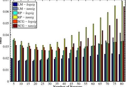
vmse. For this purpose, a parametric analysis is conducted assuming different number of neurons, different training algo-rithms and different TFs for the hidden layer of the ANNs. The number of neurons ranges from 5 to 80, assuming a step equal to 5. Moreover, three training algorithms compatible with the early stopping technique, namely the Levenberg-Marquardt (LM), the resilient back propagation (RP), and the conjugate gradient back propagation (SCG) are examined. Concerning the TF of the hidden layer, the performance of both thelogsig
and thetansig functions is evaluated. For each combination of neurons, training algorithm and TF, a set of 100 distinct initial conditions for weight and bias matrices are randomly generated by applying the Monte Carlo (MC) method. The mean values of thetmse and thevmse, provided by the MC simulations, are depicted in Figs. 8 and 9, respectively. The corresponding mean execution times are presented in Fig. 10. As shown, in all cases the training of the ANNs using the LM algorithm requires higher execution times compared to the cases when the RP and the SCG are used. However, as illustrated in Figs. 8 and 9, the LM algorithm provides the best results, i.e. the minimum values, for both the tmse and thevmse. Additionally, it is clear that the impact of the TF of the hidden layer on the performance of the ANNs is rather limited, since in all cases trivial differences are observed. However, it is interesting to note that the logsig function seems to be more suitable for this specific application, since it generally provides lower values for both thetmse and the
vmsecompared to thetansigfunction. Moreover, it is evident that the tmseis generally reduced as the number of neurons increases. This remark is valid for all the examined training algorithms and for both TFs. Concerning thevmsea different behavior is observed. Initially, as the number of neurons
2 3 4 5 6 7 8 9 10
0 0.1 0.2 0.3 0.4
Number of Clusters
WCBCR
[image:6.612.332.536.660.734.2]5 10 15 20 25 30 35 40 45 50 55 60 65 70 75 80 0
0.005 0.01 0.015 0.02 0.025 0.03 0.035
Number of Neurons
tmse
LM − logsig
LM − tansig
RP − logsig
RP − tansig
SCG − tansig
[image:7.612.329.537.55.203.2]SCG − tansig
Fig. 8. Impact of several parameters on thetmse.
5 10 15 20 25 30 35 40 45 50 55 60 65 70 75 80
0 0.01 0.02 0.03 0.04 0.05 0.06 0.07
Number of Neurons
vmse
LM − logsig
LM − tansig
RP − logsig
RP − tansig
SCG − logsig
SCG − tansig
Fig. 9. Impact of several parameters on thevmse.
increases, thevmsedecreases. However, after a certain point, a further increase in the number of neurons leads to an increase to the vmse values. This actually implies that the ANN is considerably large and thus overfits the training data [33].
The minimum vmse is observed for a number of 10 neurons, when the logsig function is used for the activation of the hidden layer and the training is performed via the LM. Hence, these settings are selected for the training of the ANNs. In this case,tmseis merely 0.0113 and the training procedure requires less than 2 s. The generalization capabilities of the proposed method are further evaluated in the next subsection.
C. Testing Procedure
The accuracy of the proposed method is evaluated here using the testing data (NT). Additionally, its performance is
compared with a conventional approach in which statistical analysis is applied to each cluster and representative parame-ters are computed by means of the corresponding mean values [10]. The execution time, required from the proposed method to derive robust model parameters for theNT data sets, was in
all cases lower that 0.1 s. This low execution time verifies the applicability of the method for close to real-time applications. Representative instances of the undertaken tests are pre-sented in Figs. 11a - 11h. More specifically, in these Figs., the real and reactive power responses, estimated by the proposed and the conventional approach, are compared with the corre-sponding laboratory measurements. The proposed method sim-ulates more accurately compared to the conventional approach
5 10 15 20 25 30 35 40 45 50 55 60 65 70 75 80
0 1 2 3 4 5 6 7 8
Number of Neurons
Time (s)
LM − logsig
LM − tansig
RP − logsig
RP − tansig
SCG − logsig
[image:7.612.71.277.56.203.2]SCG − tansig
Fig. 10. Impact of several parameters on the required execution time.
the dynamic behavior of both real and reactive power. Indeed, using the proposed method, the new steady-state and the undershoot/overshoot of real and reactive power are accurately simulated in all cases. Additionally, oscillatory responses, as the one presented in Fig. 11c, are efficiently modeled. Finally, as shown in Fig. 11e, reverse power flow phenomena that may occur during system disturbances are accurately simulated.
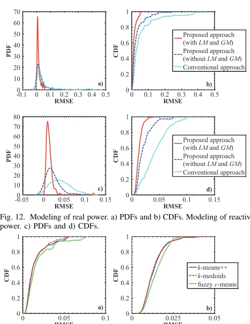
To provide a further insight in the accuracy of the proposed and the conventional approach, the probability density func-tions (PDF) and the cumulative distribution funcfunc-tions (CDF) of the RMSEs for the NT data set are presented in Fig. 12.
Concerning the modeling of the real power, PDFs indicate that the RMSE is most likely to be about 0.008 for the proposed method and 0.016 for the conventional approach. Additionally, CDFs reveal that 90% of the resulting RMSEs are under 0.039 for the proposed approach, while the corresponding percentage for the conventional approach is equal to 65%. Similar results are also observed for the modeling of the reactive power. More specifically, 90% of the resulting RMSEs for the proposed approach are lower than 0.021. On the other hand, the corre-sponding percentage for the conventional approach is merely 21%. The maximum RMSE of the proposed approach for the modeling of the reactive power is equal to 0.041. Using the conventional approach, 45% of the testing data result in higher RMSEs compared to this value. Finally, PDFs reveal that the RMSE is most likely to be about 0.011 for the proposed method and 0.034 for the conventional approach.
D. Further Investigations
In this Subsection the impact of several parameters on the accuracy of the proposed method is investigated. Initially, the impact of load and generation mix (parametersLM andGM, respectively) is evaluated. As discussed in Section III, these parameters can be assessed through forecasts or smart meter recordings. In case such data is not available or is missing, it is expected that the DSO will not be able to determine
[image:7.612.73.275.235.375.2]0 0.2 0.4 0.6 0.8 1 1.2 28 29 30 31 32 33 34 35 Time (s)
Real Power (kW)
0 0.2 0.4 0.6 0.8 1 1.2
12 14 16 18 20 22 24 26 Time (s)
Reactive Power (kVAr)
Lab Measurement Proposed Approach Conventional Approach
a) b)
0 0.2 0.4 0.6 0.8 1 1.2 1
2 3 4
Time (s)
Real Power (kW)
0 0.2 0.4 0.6 0.8 1 1.2 8 10 12 14 16 18 Time (s)
Reactive Power (kVAr)
c) d)
0 0.2 0.4 0.6 0.8 1 1.2
−1 −0.5 0 0.5 1 1.5 Time (s)
Real Power (kW)
0 0.2 0.4 0.6 0.8 1 1.2
3 3.5 4 4.5 5 5.5 Time (s)
Reactive Power (kVAr)
e) f)
0 0.2 0.4 0.6 0.8 1 1.2
−5 −4.5 −4 −3.5 −3 −2.5 Time (s)
Real Power (kW)
0 0.2 0.4 0.6 0.8 1 1.2
3 3.5 4 4.5 5 5.5 Time (s)
Reactive Power (kVAr)
g) h)
Fig. 11. Indicative responses. i) The ADN imports real power. A step-up voltage disturbance is examined. Modeling of a) real and b) reactive power. ii) The ADN imports real power. A step-down voltage disturbance is examined. Modeling of c) real and d) reactive power. iii) The ADN imports real power. A step-down voltage disturbance is examined. Bi-directional power flow is observed during the disturbance. Modeling of e) real and f) reactive power. iv) The ADN exports real power. A step-up voltage disturbance is examined. Modeling of g) real and h) reactive power.
degradation in the performance of the proposed method. Nevertheless, even in this case, the equivalent models, derived using the proposed method, are more accurate compared to the equivalents developed using the conventional approach.
The impact of the clustering technique on the accuracy of the proposed method is also evaluated. Towards this objective, the k-means++ algorithm is compared with the k-medoids and the fuzzy c-means algorithm. To provide a common comparative base, in all cases, a number of four clusters is considered. The resulting CDFs are depicted in Fig. 13. Based on these results, it is evident that the impact of the clustering method on the accuracy of the method is rather limited, since in all cases trivial differences are observed.
V. DISCUSSION ANDCONCLUSIONS
Parameters of measurement-based equivalent models can be updated only when new disturbances are available. Due to this inherent limitation, the accuracy of these models for online applications is rather limited. To address this issue, in this paper, a new method, based on artificial-intelligence
-0.10 0 0.1 0.2 0.3 0.4 0.5
10 20 30 40 50 60 70 RMSE P D F
0 0.1 0.2 0.3 0.4 0.5
0 0.2 0.4 0.6 0.8 1 RMSE C D F Proposed approach
(with LM and GM)
Proposed approach
(without LM and GM)
Conventional approach
a) b)
-0.050 0 0.05 0.1 0.15
10 20 30 40 50 60 70 80 RMSE P D F
0 0.05 0.1 0.15
0 0.2 0.4 0.6 0.8 1 RMSE C D F Proposed approach
(with LM and GM)
Proposed approach
(without LM and GM)
Conventional approach
[image:8.612.312.559.51.371.2]c) d)
Fig. 12. Modeling of real power. a) PDFs and b) CDFs. Modeling of reactive power. c) PDFs and d) CDFs.
0 0.05 0.1
0 0.2 0.4 0.6 0.8 1 RMSE C D F
0 0.025 0.05
0 0.2 0.4 0.6 0.8 1 RMSE C D
F k-means++
k-medoids
fuzzy c-means
[image:8.612.81.262.54.410.2]a) b)
Fig. 13. CDFs of the proposed method, assuming different clustering techniques. a) Modeling of real and b) reactive power.
techniques, is developed. In the proposed framework, a train-ing data set, containtrain-ing disturbance events, is used for the estimation of the required model parameters. Using the derived parameters, ANNs are trained. The ANNs aim to identify general relationships between the parameters of the adopted equivalent model and the pre-disturbance operating conditions, the load and the generation mix of the examined ADN.
During the online application, operating conditions of the ADN as well as the load and the generation mix are forwarded as inputs to the developed ANNs, which provide (without requiring new disturbance events) in close to real-time sets of model parameters that optimally describe the examined ADN. The effectiveness of the proposed method is evaluated using measurements acquired from a laboratory-scale ADN, while its performance is compared with a conventional approach. Comparison results reveal that the proposed method presents superior performance compared to the conventional one, sim-ulating more accurately the complex dynamic phenomena that occur in ADNs (i.e. oscillations, bi-directional power flows).
the training of the ANNs. Moreover, the conducted analysis reveals that a number of 10 neurons can ensure very accurate results. The above settings can be used as indicative values for the derivation of generic aggregated equivalent models.
Additionally, the impact of the clustering technique as well as the impact of load and generation mix on the accuracy of the proposed method are evaluated. Results indicate that the accuracy of the proposed method is not affected by the clustering technique used. Moreover, evaluation results reveal that input of information concerning load and generation mix of the examined ADN can enhance the accuracy of the proposed method. Nevertheless, the proposed method results in more accurate and robust models as compared to the conventional approach, even in cases where this information is not available.
Based on the evaluation results, it can be concluded that the proposed method constitutes a reliable tool that can be used from DSOs for the derivation of generic measurement-based dynamic equivalent models.
Future work will incorporate load and generation mix esti-mates of the ADN using measurements acquired at PCC with the external grid. This way, the impact of forecast errors on the accuracy of the proposed method will be eliminated.
REFERENCES
[1] S. M. Zali and J. V. Milanovic, “Generic model of active distribution network for large power system stability studies,”IEEE Trans. Power Syst., vol. 28, no. 3, pp. 3126–3133, Aug., 2013.
[2] J. V. Milanovic and S. M. Zali, “Validation of equivalent dynamic model of active distribution network cell,”IEEE Trans. Power Syst., vol. 28, no. 3, pp. 2101–2110, Aug., 2013.
[3] Cigre Report, Working Group C4.605. Modelling and aggregation of loads in flexible power networks, Feb. 2014.
[4] J. V. Milanovic and M. Kayikci, “Transient responses of distribution network cell with renewable generation,” in2006 IEEE PES Pow. Syst. Conf. and Exp., Oct., 2006, pp. 1919–1925.
[5] Z. Miao, A. Domijan, and L. Fan, “Investigation of microgrids with both inverter interfaced and direct ac-connected distributed energy resources,” IEEE Trans. Power Del., vol. 26, no. 3, pp. 1634–1642, Jul. 2011. [6] F. Katiraei, M. R. Iravani, and P. W. Lehn, “Small-signal dynamic model
of a micro-grid including conventional and electronically interfaced distributed resources,”IET Gen., Trans. Dist., vol. 1, no. 3, pp. 369– 378, May 2007.
[7] U. D. Annakkage, et al., “Dynamic system equivalents: A survey of available techniques,”IEEE Trans. Power Del., vol. 27, no. 1, pp. 411– 420, Jan. 2012.
[8] P. N. Papadopoulos, et al., “Black-box dynamic equivalent model for microgrids using measurement data,”IET Gen., Trans. Dist., vol. 8, no. 5, pp. 851–861, May 2014.
[9] B.-K. Choi, H.-D. Chiang, Y. Li, H. Li, Y.-T. Chen, D.-H. Huang, and M. G. Lauby, “Measurement-based dynamic load models: derivation, comparison, and validation,”IEEE Trans. Power Syst., vol. 21, no. 3, pp. 1276–1283, Aug., 2006.
[10] D. P. Stojanovic, L. M. Korunovic, and J. Milanovic, “Dynamic load modelling based on measurements in medium voltage distribution net-work,”Elect. Power Syst. Res., vol. 78, no. 2, pp. 228 – 238, Feb., 2008.
[11] Measurement-Based Load Modeling. EPRI, Palo Alto. CA: 2006. 1014402.
[12] K. S. Metalinos, T. A. Papadopoulos, and C. A. Charalambous, “Deriva-tion and evalua“Deriva-tion of generic measurement-based dynamic load mod-els,”Elect. Power Syst. Res., vol. 140, pp. 193–200, 2016.
[13] H. Renmu, M. Jin, and D. J. Hill, “Composite load modeling via measurement approach,”IEEE Trans. Power Syst., vol. 21, no. 2, pp. 663–672, May 2006.
[14] E. O. Kontis, T. A. Papadopoulos, A. I. Chrysochos, and G. K. Papagiannis, “Measurement-based dynamic load modeling using the vector fitting technique,”IEEE Trans. Power Syst., vol. 33, no. 1, pp. 338–351, Jan., 2018.
[15] E. O. Kontis, A. I. Chrysochos, G. K. Papagiannis, and T. A. Pa-padopoulos, “Development of measurement-based generic load models for dynamic simulations,” in 2015 IEEE Eindhoven PowerTech, Jun., 2015, pp. 1–6.
[16] A. M. Azmy,I. Erlich, andP. Sowa, “Artificial neural network-based dynamic equivalents for distribution systems containing active sources,”
IET Gener. Transm. Dis., vol.151, no.6, pp.681–688, Nov.,2004. [17] C. Changchun,et al., “Micro-grid dynamic modeling based on RBF
Ar-tificial Neural Network,” inInternational Conference on Power System Technology, Oct.2014, pp. 3348–3353.
[18] A. Arif,et al., “Load Modeling—A Review,”IEEE Trans. Smart Grid, vol.9, no.6, pp.5986–5999, Nov.2018.
[19] H. Golpira, H. Seifi, and M. R. Haghifam, “Dynamic equivalencing of an active distribution network for large-scale power system frequency stability studies,”IET Gen., Trans. Dist, vol. 9, no. 15, pp. 2245–2254, Nov. 2015.
[20] E. O. Kontis, I. S. Skondrianos, T. A. Papadopoulos, A. I. Chrysochos, and G. K. Papagiannis, “Generic dynamic load models using artificial neural networks,” in2017 52nd Int. Univ. Power Eng. Conf. (UPEC), Aug., 2017, pp. 1–6.
[21] D. Karlsson and D. J. Hill, “Modelling and identification of nonlinear dynamic loads in power systems,”IEEE Trans. Power Syst., vol. 9, no. 1, pp. 157–166, Feb., 1994.
[22] E. O. Kontis, S. P. Dimitrakopoulos, A. I. Chrysochos, G. K. Papa-giannis, and T. A. Papadopoulos, “Dynamic equivalencing of active distribution grids,” in 2017 IEEE Manchester PowerTech, Jun., 2017, pp. 1–6.
[23] E. O. Kontis, T. A. Papadopoulos, A. I. Chrysochos, and G. K. Papagiannis, “On the applicability of exponential recovery models for the simulation of active distribution networks,”IEEE Trans. Power Del., in press.
[24] B. Stephen and S. J. Galloway, “Domestic load characterization through smart meter advance stratification,” IEEE Trans. Smart Grid, vol. 3, no. 3, pp. 1571–1572, Sept., 2012.
[25] J. Liang, S. K. K. Ng, G. Kendall, and J. W. M. Cheng, “Load signature study - part i: Basic concept, structure, and methodology,”IEEE Trans. Power Del., vol. 25, no. 2, pp. 551–560, Apr. 2010.
[26] J. V. Milanovi´c and Y. Xu, “Methodology for estimation of dynamic response of demand using limited data,” IEEE Trans. Power Syst., vol. 30, no. 3, pp. 1288–1297, May 2015.
[27] I. P. Panapakidis, “Clustering based day-ahead and hour-ahead bus load forecasting models,”Int. J. Electr. Power Energy Syst., vol. 80, pp. 171– 178, 2016.
[28] S. M. Zali, N. C. Wooley, and J. V. Milanovic, “Developemnt of equivalent dynamic model of distribution network using clustering procedure,” in17th Power Syst. Computation Conf., Jun., 2011, pp. 1–8. [29] D. Issicaba, A. S. Costa, and J. L. Colombo, “Real-time monitoring of points of common coupling in distribution systems through state estimation and geometric tests,”IEEE Trans. Smart Grid, vol. 7, no. 1, pp. 9–18, Jan., 2016.
[30] G. J. Tsekouras, N. D. Hatziargyriou, and E. N. Dialynas, “Two-stage pattern recognition of load curves for classification of electricity customers,” IEEE Trans. Power Syst., vol. 22, no. 3, pp. 1120–1128, Aug. 2007.
[31] B. Gustavsen, “Improving the pole relocating properties of vector fitting,” IEEE Trans. Power Del., vol. 21, no. 3, pp. 1587–1592, Jul. 2006.
[32] D. J. Trudnowski, J. M. Johnson, and J. F. Hauer, “Making Prony analysis more accurate using multiple signals,”IEEE Trans. Power Syst., vol.14, no.1, pp.226–231,Feb. 1999.
[33] H. Demuth and M. Beale,MATLAB Neural Network Toolbox User’s Guide. Version 4.
[34] Y. Xu and J. V. Milanovi´c, “Artificial-intelligence-based methodology for load disaggregation at bulk supply point,” IEEE Trans. on Power Syst., vol. 30, no. 2, pp. 795–803, Mar, 2015.
[35] “Load representation for dynamic performance analysis (of power sys-tems),”IEEE Trans. Power Syst., vol. 8, no. 2, pp. 472–482, May 1993. [36] J. Liu and C. Chu, “Long-term voltage instability detections of mul-tiple fixed-speed induction generators in distribution networks using synchrophasors,”IEEE Trans. Smart Grid, vol. 6, no. 4, pp. 2069–2079, Jul. 2015.