An Eigenvalue-based Approach for Structure
Classification in Polarimetric SAR Images
Filippo Biondi,
Member, IEEE
, Carmine Clemente,
Senior Member, IEEE
, and Danilo Orlando,
Senior Member,
IEEE
Abstract—In this paper, we design a novel unsupervised archi-tecture for automatic classification of the dominant polarization in polarimetric SAR images. To this end, we leverage the ideas developed in [1] and suitably exploit them to build a decision logic capable of recognizing the dominant scattering mechanism which characterizes the pixel under test. Specifically, we combine the original data to generate three different sets of reduced-size vectors, which feed a dominant eigenvalues classifier based upon the Model Order Selection rules. Then, the outputs of the latter classification schemes are exploited to infer, according to a specific criterion, the dominant polarization. The performance analysis is conducted on measured data and points out the effectiveness of the newly proposed classification architecture also showing that information about the dominant polarization can be representative of the type of structure which gives raise to the dominant backscattering mechanism.
Index Terms—Covariance matrix, eigenvalues decomposition, model order selection rules, polarimetric SAR image classifica-tion, structure classification.
I. INTRODUCTION
Polarimetric Synthetic Aperture Radar imaging (PolSAR) has been demonstrated to have the capability to provide highly reliable and valuable information for remote sensing [2]–[5], allowing advanced discrimination and understanding of the imaged scene. This radar imaging sensor acquires information from a scene when vertical or horizontal polarization is trans-mitted and/or received. Scattering mechanisms that rule the de-polarization effect can be then identified and used to infer about the observed scene. The exploitation of SAR polarimetry is of particular relevance in civilian and defence applications. In this former context, extended area monitoring and target areas classification receive the widest attention by researchers. A non-exhaustive list of applications of polarimetric SAR in remote sensing includes biomass estimation [6], rice paddy monitoring [7], snow and ice analysis [8], oil spill detec-tion [4], land-use classificadetec-tion [9], crop monitoring, damage assessment, deforestation, flood delineation, burn mapping, disaster management, urban mapping and others [10].
In the classification context, the information extracted from the polarimetric channels is typically used to characterize different portions of the acquired scene in an automatic or semi-automatic way [10]–[14]. Generally speaking, existing strategies for scene classification from SAR images can be
Filippo Biondi is with Italian Ministry of Defence. E-mail: biopippo@gmail.com.
Carmine Clemente is with the Centre for Signal and Image Processing, De-partment of Electronic and Electrical Engineering, University of Strathclyde, G1 1XW, Glasgow.E-mail: carmine.clemente@strath.ac.uk.
D. Orlando is with Universit`a degli Studi “Niccol`o Cusano”, 00166 Roma, Italy.E-mail: danilo.orlando@unicusano.it.
grouped into two main categories, namely unsupervised and supervised algorithms, and have been extensively investigated [9], [12], [15]–[21]. The former consists of clustering image pixels by means of common characteristics/features and occurs in an automatic way without any kind of aid from the user. On the other hand, the latter exploits training pixels, which are a-priori selected by the user to define the features identifying a specific class [15], [16]. In [1], the problem of estimating the number of dominant covariance eigenvalues (which are representative of the scattering mechanisms) in polarimetric SAR images was investigated assuming that the polarimetric image pixels share the same covariance but different power levels.
In this paper we propose a novel unsupervised approach to classify dominant polarizations in polarimetric SAR im-ages. Specifically, it suitably extends the Dominant Eigenvalue Classification Scheme (DECS) proposed in [1] by integrating reduced sized classifiers based upon Model Order Selection (MOS) rules [22]. All the classification outcomes are then processed by a decision logic able to identify the dominant polarization in a pixel1. The effectiveness of the proposed framework is demonstrated on real PolSAR data in which manmade structures and vegetation have been identified. The expected returned dominant polarization can be intuitively inferred through general knowledge of the electromagnetic scattering mechanism. The results show the capability of the proposed approach to classify correctly the dominant polariza-tion in all the investigated cases. Remarkably, they can feed a further processing stage for automatic target recognition, land use classification, etc. without the intervention of a human operator.
The remainder of the paper is organized as follows2: Section II introduces the problem formulation, the classification archi-tecture is described in Section III. The analysis on real PolSAR data is reported in Section IV. Finally, Section V contains some concluding remarks and outlines future research tracks.
1Note that algorithm proposed in [1] can only identify the order relations
existing between the eigenvalues of the polarimetric covariance matrix without providing any information about the dominant polarization.
2The adopted notation uses boldface for vectorsa(lower case) and matrices
A (upper case). The trace and the determinant of a square matrix are denoted by tr(·)anddet(·), respectively, whereas(·)†indicates the conjugate
transpose. Symbol0denotes the the null vector with suitable size, whilek · k
is the Euclidean vector norm. Finally,x∼ CNN(m,M)means thatxis
II. DATACUBECONSTRUCTION ANDPRELIMINARY
DEFINITIONS
A polarimetric SAR image, assuming a monostatic SAR acquisition mode, is a (L×M)-dimensional matrix whose entries are 3-dimensional complex vectors. Each component of these vectors represents the returns acquired by a specific polarimetric channel, namely HH channel for the first compo-nent, HV channel for the second compocompo-nent, and VV channel for the third component. Therefore, the sensor provides a 3-D data stack of size L×M ×3 which is referred to in the following as datacube.
The classification problem addressed here is aimed at iden-tifying the dominant polarimetric component for each pixel of the datacube. This information can be used to infer the kind of structures present in the observed scene. To this end, for the generic pixel under test, a rectangular neighborhood3 A of size K ≥N is extracted and a suitable function of these vectors is devised for classification purposes. For simplicity, let us denote the elements ofAbyxi,i= 1, . . . , K, and assume that xi ∼ CN3(0, σ2iC), where C is the positive definite covariance matrix structure and σi > 0 is a scaling factor [13]. Note that σi is representative of the reflectivity strength of each pixel.
Finally, the classification problem at hand can be written as
H1: Ais characterized by the VV polarization,
H2: Ais characterized by the HH polarization,
H3: Ais characterized by the HV polarization.
(1)
In the next section, we devise a classification architecture to solve the above ternary hypothesis test which takes advantage of the hidden information carried by the polarimetric vectors.
III. DESIGN OF THECLASSIFICATIONARCHITECTURE ANDPARAMETERESTIMATION
The herein proposed procedure leverages the ideas devel-oped in [1] and suitably enriches them to obtain a decision logic capable of recognizing the dominant polarization of the scattering events represented by A. Specifically, in [1], the authors consider the following multiple hypothesis test
H1:λ1=λ2=λ3=λ,
H2:λ1≥λ2=λ3,
H3:λ1=λ2≥λ3,
H4:λ1≥λ2≥λ3,
(2)
where λ1 ≥ λ2 ≥ λ3 are the eigenvalues of C arranged in
decreasing order (note that the above hypothesis test contains nested hypotheses sinceH2⊂H4andH3⊂H4), and propose
a classification scheme (DECS), which identifies the dominant covariance eigenvalues. This preliminary information can be exploited to infer the dominant polarization. As a matter of fact, ifH2orH3are selected, then an eigenvalue classification
scheme can be applied to new reduced-size vectors obtained by considering suitable 2-dimensional combinations of the com-ponents of the original vectors. In this case, the classification
3In order not to burden the notation, in the following we omit the subscript
of the generic pixel under test.
problem is binary and each eigenvalue is associated with a specific polarization. Finally, these classification results can be jointly used to establish the dominant polarization.
Summarizing, the resulting architecture can be obtained by adding a new branch to the processing chain of DECS. Such branch is formed by cascading a reduced-size eigenvalue classifier and a decision scheme which combines previously selected hypotheses to choose the dominant polarization.
Let us begin from the reduced-size classifier and consider a generic pixel under test along with the set of surrounding vectors, x1, . . . ,xK say. As previously stated, the entries of xi contain the responses of the polarimetric channels in a specific order, namely xi = [xi,HH xi,HV xi,V V]T ∼
CN3 0, σi2C
, where xi,AB ∈ C is the component cor-responding to the AB polarization with A, B ∈ {H, V}. Now, in order to compare the polarization strength each other, for each polarimetric vector, we consider all the 2 -combinations of the three original components to construct the following 2-dimensional vectors xi,a = [xi,HH xi,V V]
T
∼ CN2(0, σi2Ca), xi,b = [xi,HH xi,HV]
T
∼ CN2(0, σ2iCb), and xi,c = [xi,V V xi,HV]
T
∼ CN2(0, σi2Cc), where a =
HHV V,b=HHHV, andc=V V HV. Moreover,Ca,Cb, andCc are obtained by removing the second, the third, and first row and column fromC, respectively. Thus, we deal with three sets of data.
Following the lead of [13], we can remove the de-pendence on σ2
i by dividing each vector with respect to the respective Euclidean norm to obtain zi,a =
xi,a
kxi,ak, zi,b =
xi,b
kxi,bk, and zi,c =
xi,c
kxi,ck, whose
probability density function (pdf) can be written as [1]
f(Zy;Cy) = [det (Cy)]− KQK
i=1
tr C−y1Si,y
−2
, where
Zy ∈ [z1,y, . . . ,zK,y], y ∈ {a, b, c}, and Si,y = zi,yz†i,y. The classifier, fed by the transformed data, selects one of the following hypotheses
∀y∈ {a, b, c}:
(
H1,y: λ1,y=λ2,y=λy,
H2,y: λ1,y≥λ2,y,
(3)
where λk,y > 0, k = 1,2, are the eigenvalues4 of Cy. To this end, we resort to the MOS rules [22] whose expression contains a fitting term represented by the compressed log-likelihood under each hypothesis and a penalty term depending on the number of unknown parameters. The former can be written noticing that
1) underH1,y: the likelihood function does not depend on
the unknown parameterλy. In fact, it is possible to show
that f(Zy;Cy) =Q K i=1
kzi,yk
2−2
= 1;
2) under H2,y: the Maximum Likelihood Estimate ofCy,
b
Cysay, is the fixed point ofCy= K2
PK
i=1
zi,yz†i,y
z†
i,yC
−1 y zi,y
and, hence, the expression of the compressed log-likelihood is logf(Zy;Cby) = −Klog det
h b Cy
i
−
2PK
i=1logtr h
b C−y1Si,y
i
.
4It is worth recalling that the eigenvalues of the covariance matrix provide
As for the penalty factor, the number of unknown parameters under H1,y is 0, while underH2,y, the number of unknown parameters is3.
Gathering the above results, the expression of the MOS-based classifier is given by
Hˆi,y= arg max
{H1,y,H2,y}
n
−2 logf(Zy;Cby) +ηkp(i)
o
, (4)
wherekp(i)is the number of unknown parameters under the
Hi,i= 1,2, hypothesis, andη= 2for AIC,η= 1 +ρ, ρ≥1 for GIC, and η = logK for BIC. The acronyms AIC, BIC, and GIC stand for Akaike Information Criterion, Bayesian Information Criterion, and Generalized Information Criterion, respectively [22]. The above classifier is referred to in the following as RS-DECS. Finally, denote by λˆi,y, i = 1,2,
y =a, b, c, the eigenvalues of Cby, then the decision scheme that combines the information provided by the considered classifiers returns the dominant polarization according to the following line of reasoning:
• HH is selected as the dominant polarization if: DECS returns H2 and (H2,a, H2,b, H1,c) hold; DECS returns
H3 and (H2,a, H2,c, H1,b)hold and ˆλ1,a >ˆλ1,c; DECS
returns H3 and(H2,b, H2,c, H1,a)hold andλˆ1,b>λˆ1,c;
• HV is selected as the dominant polarization if: DECS returns H2 and (H2,b, H2,c, H1,a) hold; DECS returns
H3 and (H2,a, H2,c, H1,b)hold and ˆλ1,a <ˆλ1,c; DECS
returns H3 and(H2,a, H2,b, H1,c)hold andλˆ1,b>λˆ1,a;
• VV is selected as the dominant polarization if: DECS returns H2 and (H2,a, H2,c, H1,b) hold; DECS returns
H3 and (H2,b, H2,c, H1,a) hold andλˆ1,b <ˆλ1,c; DECS
returns H3 and(H2,a, H2,b, H1,c)hold andλˆ1,b<λˆ1,a.
The entire architecture is depicted in Figure 1, where Z =
h x
1
kx1k, . . . ,kxxKKk
i
and Hb is the hypothesis selected by the
preliminary stage represented by DECS. The RS-DECS stages return Hby ∈ {Hi,y : i= 1,2, y=a, b, c}, which are, then, used by the final stage to identify the dominant polarization5.
IV. NUMERICALEXAMPLES, DISCUSSION,AND
PERFORMANCE
In this section, we investigate the performance of the proposed architecture over three different regions of interest (ROIs) drawn from SAR data collected by an unmanned aerial vehicle synthetic aperture radar of the United States National Aeronautics and Space Administration. This air-borne system owns full-polarimetic SAR capabilities and works in the L-band with a range-azimuth resolution of 5 meters. Moreover, the look direction is left, the acquisition heading is 85.754562◦, and the altitude is 0.12 · 105 m. For additional details, the interested reader is referred to the metadata file “SanAnd-08519-14145-008-141009-L090-CX-01.ann”. In fact, we exploit the SAR image with ID num-ber6 SanAnd-08519-14145-008-141009-L090-CX-01. Specif-ically we consider the areas reported in Figures 2 and
5Note that in the case of a polarization basis transformation, the processing
scheme returns the dominant component which is related to the original dominant polarization through a one-to-one transformation.
6The reader is referred to
https://www.asf.alaska.edu/about/how-to-cite-data/ for data downloading.
3. The triangle labeled P1 in each figure represent a ref-erence point useful to select the considered areas. This point is geolocated at the coordinates (Datum world geode-tic system 1984 European petroleum survey group 4230) lat:33.855028◦ N, lon: 116.568656◦ W for Figure 2. The reference point P1 of Figure 3 is geolocated at the following coordinates: lat:33.820785◦N, lon:116.503983◦W. The set
A is formed by selecting the pixels belonging to a square window of size 5×5 and centered on the pixel under test. Moreover, DECS and RS-DECS incorporate BIC since it does not require any additional tuning parameter and provides excellent classification capabilities as shown in [1].
The considered ROIs are indicated in Figure 2 through two yellow squares labeled1 and2. In the detail, ROI 1 contains vertical structures represented by the wind turbines of Palm Springs wind farm, whereas in ROI 2 the vertical structures are associated with a train. Finally, the ROI 3 is reported in Figure 3 and contains horizontal structures associated with airport landing strips.
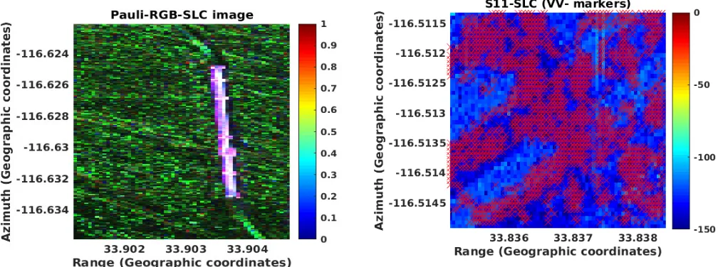
Let us begin by applying the classification scheme to ROIs1 and2where the predominant structures are vertical. The Pauli-RGB magnitude of a portion of ROI 1 corresponding to some big wind turbines of the Palm Springs wind farm is shown in Figure 4, where the vertical structures are represented by the small bright regions. The classification performance of the proposed architecture can be found in Figure 5. Note that the colorbars represent an indication of (possibly the logarithm of) the normalized pixel energy. Inspection of the figure highlights that the latter correctly selects the VV polarization (yellow cross markers) as the dominant component in the areas where the wind turbines (which yield double-bounces) are present. To be more quantitative, the proposed method identifies all the 26 turbines belonging to the considered region with 0 false alarms. The image containing the yellow markers is superimposed to the SLC image in magnitude representing the single polarimetric channel s11. The Pauli-RGB magnitude image of ROI 2 is shown in Figure 6, where the bright vertical strip represents a train. The classification results are shown in Figure 7 where the red cross markers indicating the VV polarization are displaced along the boundary of the train, namely in correspondence with the vertical metallic structures. Again, the image containing the markers is superimposed to the SLC image in magnitude representing the single polarimet-ric channel s11. Note that the markers seem slightly shifted in range due to the layover and double-bounce scattering effects taking place because of the slant characteristic of the SAR acquisition geometry.
V. CONCLUSIONS
In this paper, we focused on the problem of dominant polarization classification in polarimetric SAR images. To this end, the hidden information enclosed in the polarimetric data has been extracted by creating reduced-size vectors which allowed to classify the dominant eigenvalue for each pair of polarizations. Then, this information has been exploited by a decision logic to infer the resulting dominant polarization. The numerical examples, carried out on measured polarimetric SAR data, have highlighted that the proposed classification architecture can correctly recognize the dominant scattering mechanisms associated with the structures present in the observed scene. Future research might consider the design of object/target recognition algorithms for low-resolution images which take advantage of the information provided by the herein proposed classification architecture.
REFERENCES
[1] L. Pallotta and D. Orlando, “Polarimetric Covariance Eigenvalues Classification in SAR Images,” IEEE Geoscience and Remote Sensing Letters, pp. 1–5, 2018.
[2] D. Giuli, “Polarization Diversity in Radars,” Proceedings of the IEEE, vol. 74, no. 2, pp. 245–269, February 1986.
[3] L. M. Novak, M. B. Sechtin, and M. J. Cardullo, “Studies of target detection algorithms that use polarimetric radar data,”IEEE Transactions on Aerospace and Electronic Systems, vol. 25, no. 2, pp. 150–165, 1989. [4] A. De Maio, D. Orlando, L. Pallotta, and C. Clemente, “A Multifamily GLRT for Oil Spill Detection,”IEEE Trans. on Geoscience and Remote Sensing, vol. 55, no. 1, pp. 63–79, January 2017.
[5] C. Hao, S. Gazor, X. Ma, S. Yan, C. Hou, and D. Orlando, “Polarimetric detection and range estimation of a point-like target,”IEEE Transactions on Aerospace and Electronic Systems, vol. 52, no. 2, pp. 603–616, April 2016.
[6] M. C. Dobson, F. T. Ulaby, L. E. Pierce, T. L. Sharik, K. M. Bergen, J. Kellndorfer, J. R. Kendra, E. Li, Y. C. Lin, A. Nashashibi, K. Sara-bandi, and P. Siqueira, “Estimation of forest biophysical characteristics in Northern Michigan with SIR-C/X-SAR,” IEEE Transactions on Geoscience and Remote Sensing, vol. 33, no. 4, pp. 877–895, July 1995. [7] J. M. Lopez-Sanchez, S. R. Cloude, and J. D. Ballester-Berman, “Rice Phenology Monitoring by Means of SAR Polarimetry at X-Band,”IEEE Transactions on Geoscience and Remote Sensing, vol. 50, no. 7, pp. 2695–2709, July 2012.
[8] J. Shi and J. Dozier, “Inferring snow wetness using C-band data from SIR-C’s polarimetric synthetic aperture radar,” IEEE Transactions on Geoscience and Remote Sensing, vol. 33, no. 4, pp. 905–914, July 1995. [9] P. Addabbo, F. Biondi, C. Clemente, D. Orlando, and L. Pallotta, “Classification of covariance matrix eigenvalues in polarimetric SAR for environmental monitoring applications,”IEEE Aerospace and Electronic Systems Magazine (accepted to), January 2019.
[10] J. S. Lee and E. Pottier, Polarimetric Radar Imaging: From Basics to Applications, CRC Press, 2009.
[11] L. Ferro-Famil and E. (Editor in Chief J. A. Kong) Pottier, Progress In Electromagnetics Research, vol. 24, chapter Dual Frequency Polari-metric SAR Data Classification and Analysis, pp. 251–276, New York Elsevier, 2001.
[12] L. Pallotta, C. Clemente, A. De Maio, and J. J. Soraghan, “Detecting Covariance Symmetries in Polarimetric SAR Images,” IEEE Transac-tions on Geoscience and Remote Sensing, vol. 55, no. 1, pp. 80–95, January 2017.
[13] L. Pallotta, A. De Maio, and D. Orlando, “A Robust Framework for Covariance Classification in Heterogeneous Polarimetric SAR Images and Its Application to L-Band Data,”IEEE Transactions on Geoscience and Remote Sensing, vol. 57, no. 1, pp. 104–119, Jan 2019.
[14] S. Tahraoui, C. Clemente, L. Pallotta, J. J. Soraghan, and M. Ouarzed-dine, “Covariance Symmetries Detection in PolInSAR Data,” IEEE Transactions on Geoscience and Remote Sensing, vol. 56, no. 12, pp. 6927–6939, Dec 2018.
[15] J. S. Lee, K. P. Papathanassiou, I. Hajnsek, T. Mette, M. R. Grunes, T. L. Ainsworth, and L. Ferro-Famil, “Applying Polarimetric SAR Interferometric Data for Forest Classification,” inIEEE International Geoscience and Remote Sensing Symposium (IGARSS). IEEE, 2005, vol. 7.
[16] S. Uhlmann and S. Kiranyaz, “Evaluation of Classifiers for Polarimetric SAR Classification,” in IEEE International Geoscience and Remote Sensing Symposium (IGARSS). IEEE, 2013, pp. 775–778.
[17] J. J. Van Zyl, “Unsupervised Classification of Scattering Behavior Using Radar Polarimetry Data,”IEEE Transactions on Geoscience and Remote Sensing, vol. 27, no. 1, pp. 36–45, January 1989.
[18] J. S. Lee, M. R. Grunes, T. L. Ainsworth, L. J. Du, D. L. Schuler, and S. R. Cloude, “Unsupervised Classification Using Polarimetric Decomposition and the Complex Wishart Classifier,” IEEE Trans. on Geoscience and Remote Sensing, vol. 37, no. 5, pp. 2249–2258, September 1999.
[19] L. Ferro-Famil, E. Pottier, and J. S. Lee, “Unsupervised Classification of Multifrequency and Fully Polarimetric SAR Images Based on the H/A/Alpha-Wishart Classifier,”IEEE Trans. on Geoscience and Remote Sensing, vol. 39, no. 11, pp. 2332–2342, November 2001.
[20] J. S. Lee, M. R. Grunes, E. Pottier, and L. Ferro-Famil, “Unsupervised Terrain Classification Preserving Polarimetric Scattering Characteris-tics,” IEEE Trans. on Geoscience and Remote Sensing, vol. 42, no. 4, pp. 722–731, April 2004.
[21] N. Zhong, W. Yang, A. Cherian, X. Yang, G. S. Xia, and M. Liao, “Un-supervised Classification of Polarimetric SAR Images via Riemannian Sparse Coding,” IEEE Trans. on Geoscience and Remote Sensing, vol. 55, no. 9, pp. 5381–5390, September 2017.
[image:4.612.362.509.352.423.2][22] P. Stoica and Y. Selen, “Model-order selection: A review of information criterion rules,” IEEE Signal Processing Magazine, vol. 21, no. 4, pp. 36–47, 2004.
[image:4.612.353.523.464.564.2]Fig. 1. Block scheme for the proposed classification architecture.
Fig. 2. Orthorectified polarimetric Pauli color coded SAR image of the area containing the wind-farm and the train (rectangle boxes 1 and 2, respectively).
[image:4.612.352.524.612.709.2]Fig. 4. Pauli-RGB image for ROI 1.
[image:5.612.53.297.65.247.2]Fig. 5. Classification results for ROI 1 overlapped by the respective Pauli-RGB image: the yellow cross markers represent the VV polarization.
Fig. 6. Pauli-RGB image for ROI 3.
[image:5.612.52.291.294.479.2]Fig. 7. Classification results on ROI 3 overlapped by the respective Pauli-RGB image: the red cross markers represent the VV polarization.
Fig. 8. Pauli-RGB image for ROI 5.
[image:5.612.314.557.299.482.2] [image:5.612.55.559.529.717.2]