1
Gravitational Thermal Flows of Liquid Metals in 3D Variable
Cross-section Containers:
Transition from low-dimensional to high-dimensional chaos
Marcello Lappa1 and Hermes Ferialdi
1Department of Mechanical and Aerospace Engineering, University of Strathclyde, James Weir
Building, 75 Montrose Street, Glasgow, G1 1XJ, UK – email: [email protected]
This study extends the numerical results presented in past author’s work (Lappa and Ferialdi, Phys. Fluids, 29(6), 064106, 2017) about the typical instabilities of thermogravitational convection (the so-called Hadley flow) in containers with inclined (converging or diverging) walls. The flow is now allowed to develop along the third dimension (z). In a region of the space of parameters where the two-dimensional solutions were found to be relatively regular in time and with a simple structure in space (supporting transverse waves propagating either in the downstream or in the upstream direction), the 3D flow exhibits either waves travelling along the spanwise direction or spatially disordered and chaotic patterns. In order to identify the related mechanisms, we analyse the competition between hydrodynamic and hydrothermal (Oscillatory Longitudinal Roll) modes of convection for different conditions. A peculiar strategy of analysis is implemented, which, on the one hand, exploits the typical properties of systems developing coexisting branches of solution (“multiple” states) and their sensitivity to a variation of the basin of attraction and, on the other hand, can force such systems to select a specific category of disturbances (by enabling or disabling the related “physical” mechanisms). It is shown that hydrodynamic modes can produce early transition to chaos. The dimensionality of such states is investigated through evaluation of the “fractal” (correlation) dimension on the basis of the algorithm by Grassberger and Procaccia. When low-dimensional chaos is taken over by high-dimensional chaos, the flow develops a recognisable interval of scales where turbulence obeys the typical laws of the so-called “inertial range” and produces small-scale features in agreement with available Kolmogorov estimates.
Key words: Buoyancy flow, Lateral heating, liquid metals, non-parallel flow, Instability and bifurcation in Fluid Dynamics.
2
1. Introduction
Non isothermal flows of liquid metals induced by buoyancy are omnipresent in engineering and related technological applications (Okano et al.,1; Delgado Buscalioni and Crespo del Arco2; Kaddeche et al.,3; Li, Peng, Wu, Imaishi and Zeng4; Jaber and Saghir5; Lappa6). The related hierarchy of bifurcations and mechanisms of transition to chaos also constitute a significant and relevant part of the problem.
As an example, they have a significant impact on the solidification of industrial castings and ingots. The quality and mechanical properties of such products are adversely affected by such flows as they can produce “defects” such as channels and freckles in the material structure (Ludwig et al.,7; Abhilash et al.,8). In other circumstances, convection has just the opposite effect, i.e. it can be employed for melt homogenization and prevention of slab macroscopic irregularities (such as the entrapment of bubbles or other non-metallic inclusions). Often such casting processes rely on liquid metal compartments equipped with “baffles”, which cause a significant departure of the effective geometry from the classical rectangular solidification chamber often assumed in related numerical studies.
Flows of liquid metals and their oscillatory or chaotic states also affect the production of crystals of semiconductor or superconductor materials (in the context of “crystal-growth-from-the-melt” techniques, e.g., the horizontal Bridgman (HB), the Floating zone (FZ) or the Czochralski (CZ) technique). Leaving aside for a while the differences among such production techniques (differing essentially in the shape of the container using to host the liquid and/or in the shape of the resulting crystallized material, see, e.g., Lappa9), all such methods share a common feature, that is the presence of flow of gravitational (buoyancy) nature in the liquid undergoing solidification. Such flows can have detrimental effects on the perfection and purity of the ordered crystalline structures of the resulting solidified material (typically emerging at the micro or macro scale in the form of “striations” or “segregations”, respectively; Dupret and Van der Bogaert10; Monberg11). Actual geometries in practice are often found to have shapes with top or bottom boundaries being more or less inclined with respect to the horizontal.
3
new generation of mini-channel exchangers based on metals that are liquid at ambient temperature (or have a small melting point temperature) is being developed (Luo and Liu14).
Despite the relevance of these flows to a variety of problems, the literature on such a subject, however, seems to be still relatively limited. Most of existing studies, indeed, have been limited to two-dimensional configurations for which the dominant disturbances causing transition to time-dependent convection are expected to be purely hydrodynamic in nature.
Nevertheless, lines of evidence exist indicating that the emerging flow might have a remarkable 3D nature in many circumstances. Along these lines, as an example, Hart15,16 was the first to determine the sensitivity of this kind of convection (under the assumption of infinite layer i.e. “parallel flow”) to both transverse (2D) and longitudinal (3D) disturbances. Later, Gill17 concentrated specifically on the latter disturbances. These initial studies revealed that while the transversal instability is driven by the mean shear stress (this is the reason why it is often referred to as "shear instability" and the related disturbances as hydrodynamic one), the longitudinal instability involves dynamical coupling between the mean shear stress and the buoyancy force (a dynamical balance that makes thermal effects directly relevant to the instability mechanism, from which the denomination of “hydrothermal disturbances”).
In terms of patterning behaviour, the outcomes of these instabilities are different as well. In the first case 2D circulations appear close to the inflection point of the basic velocity profile. These perturbation rolls are therefore perpendicular to the basic flow. The latter mode of convection is featured by a pair of gravitational waves traveling in the spanwise direction. This means that the axis of the perturbation rolls is parallel to the basic flow. In practice, these longitudinal rolls combine with the basic parallel flow to produce helical trajectories of the fluid particles (from which the denomination of “Helical wave” or OLR mode, where OLR stands for “oscillatory longitudinal rolls”).
Other (later) studies have been instrumental in clarifying that the ranges of existence of the different modes of oscillatory instability determined for the infinite horizontal layer might not be directly applicable to real situations.
As an example, assuming ideally a fluid with zero Prandtl numberfluid, Afrid and Zebib18 found that the extension ofa classical rectangular geometry (with horizontal top and bottom walls) along the direction perpendicular to the basic flow can have an important effect on transition tooscillatory convection (it was shown that reducing this extensionfrom two to one could cause a significant increase in the value of the critical Rayleigh number). A similar trend was also observed in experiments (see, e.g., Hung and Andereck19 and Pratte and Hart20 for Pr=0.026). Remarkably, the latter authors found longitudinal waves to be the preferred mode of oscillatory convection in proximity to the critical threshold.
4
been specific experimental works considering the possible interplay of these two fundamental modes of convection. For instance, four “new” modes of oscillation were reported in the study by Braunsfurth and Mullin22 for Pr spanning the interval 0.016 Pr0.022. Similarly, by investigating numerically the onset of oscillations as a function of the cavity aspect ratio and Pr in the range 0Pr0.027, Wakitani23observed an increase in the value of the critical Rayleigh number for larger Pr and/or by reducing of the spanwise aspect ratio. These variations were not regular, which may be regarded as evidence of the competition of different oscillatory modes at onset.
Due to such disorganized manifestations, these convective regimes have so far resisted a deeper analysis. The problem is even more complex than as discussed above if one considers that, following the original model introduced by Hadley24, most of past efforts have been devoted to geometrical domains with relatively simple shapes (cubic or parallelepipedic enclosures with straight horizontal and vertical walls and temperature gradient perpendicular to gravity).
For relevant work where this constraint has been removed, the reader may consider the numerical studies by Delgado-Buscalioni and co-workers. As an example, Delgado-Buscalioni25,26 illustrated that, when the system is inclined, new types of instabilities can be enabled; examples along these lines being represented by the Stationary Longitudinal long-wavelength instability (SLL) and the Oscillatory Transversal long-wavelength instability (OTL). While the first may be regarded as a close relative of a classical Rayleigh-Bénard mode, the second is essentially a kind of standing wave with a rather long wavelength appearing only if the cavity is inclined and heated from below. Owing to these studies, it is also known that the inclination can even alter the properties of the typical modes of convection of the Hadley flow, namely the aforementioned hydrodynamic and hydrothermal disturbances. For instance, the stationary transverse rolls (the 2D hydrodynamic instability), that for horizontal configurations are generally observed for fluids with Pr<<1 and are suppressed for Pr>0.1 can become unstable even in gases (Pr1, Delgado-Buscalioni25). Moreover, the OLR instability is damped at a certain cutoff value of Pr, which increases with the inclination angle with respect to the horizontal direction () (e.g, for =0° and 10° OLR perturbations are damped for Pr0.21 and Pr0.26, respectively, Delgado-Buscalioni26).
Despite these remarkable results, only in the last couple of years, however, has the importance of the different inclination of the walls been realised. As an example, most recently, the ability of oppositely inclined walls (delimiting the fluid from above and from below) to further expand the set of convective modes potentially excitable when the Rayleigh number is increased has been shown by Lappa and Ferialdi27 under the constraint of 2D flow. These systems may be regarded as an additional variant, for which though the top and bottom walls are not horizontal, no net inclination is present as these boundaries are one the mirror image of the other. Thereby, a new line of inquiry in the study of these subjects has been opened up for cases in which, though the system is not tilted, the widespread assumption of “parallel flow” is no longer applicable.
5
converging or diverging walls in the xy (basic flow) plane and different spanwise aspect ratios (assuming either periodic boundary conditions or solid walls as limiting condition along the z axis).
2. Mathematical Model and Numerical Method
2.1 The System
As shown in Fig. 1, the considered three-dimensional shallow cavity is symmetric with respect to the horizontal x axis. Such a configuration is laterally delimited along x by solid walls at different temperatures (one heated, the other cooled, having height dhot and dcold, respectively). Moreover,
with regard to the other direction (z axis in Fig. 1) we focus on two possible situations, i.e. vertical adiabatic walls or periodic boundary conditions (to mimic an infinite extension along that direction). This naturally leads to three different non-dimensional (independent) parameters characterizing such a problem, namely the streamwise (or transverse) aspect ratio Ax, defined as the cavity
length-to-average-depth ratio Ax=L/d where d = (dhot + dcold)/2, the spanwise (or longitudinal) aspect ratio,
Az=W/d (where W is the extension of the computational domain along z) and the so-called
expansion (compression) ratio =dhot/dcold27.
[image:5.595.109.490.409.614.2]For all cases, we assume the top and bottom walls to be adiabatic (no heat exchange).
Fig. 1: Sketch of the considered geometry and related thermal and kinematic boundary conditions.
6
As preliminarily shown by Lappa and Ferialdi28, the properties of this unicellular basic flow are very sensitive to the value of the parameter . More specifically, both the streamfunction and the nondimensional shear stress attain a minimum when =1, i.e. when the top and bottom walls are perfectly horizontal and increase as soon as becomes 1. When the Rayleigh number is increased, under the constraint of two-dimensionality27 such a flow can undergo shear driven instabilities leading to a variety of possible waveforms.
Our article builds on, but also seeks to extend, such earlier works by expressly targeting an improved understanding of the regimes of fluid motion that can be established in such configurations when the constraint of two-dimensional flow is removed and the Rayleigh number is increased. Such a parameter is defined here as:
Ra=GrPr=gTTd3/ (1)
where T is the horizontal temperature difference, is the thermal diffusivity, is the kinematic viscosity, T is the thermal expansion coefficient, Pr=/ the Prandtl number, Gr=Ra/Pr the
Grashof number.
In past linear stability analyses on the subject (for the case of horizontal parallel flows), hydrodynamic and hydrothermal disturbances were observed as the preferred (most critical) perturbations for Pr=O(10-2) and Pr=O(10-1), respectively. For systems featuring a net inclination with tilts similar to those considered in the present work (though with opposite sign for the top and bottom boundaries), such modes were found to interact (codimension-two point) for Pr located in a certain neighbourhood of Pr=0.03 (see Delgado-Buscalioni25). Accordingly, in the present analysis we consider Pr=0.01 and Pr=0.05. Moreover, as in Ref27, we assume Ax= 10.
2.2 Governing Equations
The governing equations for mass, momentum and energy, properly cast in nondimensional form read:
0
V (2)
VV V Ra T igp t
V
Pr Pr2
(3)
VT T tT 2
(4)
where V (u,v,w), T and p are the nondimensional velocity, temperature and pressure, respectively, ig
7
the buoyancy production term in the momentum equation. Velocity and temperature have been referred to the scales /d and T, respectively and all distances have been scaled on d.
2.3 The Numerical Method
Our solution procedure for the governing equations is based on a classical Finite Volume Method (FVM) strategy, which means that the integral form of such equations is discretized over a finite set of control volumes. The algorithm is articulated into different stages as required by the so-called PISO (Pressure-Implicit Split Operator) approach (Jang et al.,29, Yen and Liu30). This technique may be regarded as a variant of the general class of techniques pertaining to the category of projection methods (also known under several other names such as: fractional-step method or pressure-correction method, also simply referred to as primitive-variables approach). Such denomination reflects the intrinsic nature of the coupling between velocity and pressure. These two quantities are treated in an apparently segregated manner. Overall, this method may be regarded as a numerical spin off of the so-called inverse theorem of the vector calculus (Ladyzhenskaya32). From a theoretical point of view, a simple sketch of it may be provided as follows: Initially a provisional velocity field V* is determined neglecting the influence of pressure. This results in a field that satisfies the balance equation for the vorticity (equation derived by applying the curl operator to the momentum equation). In a subsequent step, pressure is determined via an additional equation derived from the continuity equation. The provisional velocity field is finally corrected via the gradient of such pressure thereby making it compliant with the requisite of incompressible flow. In practice, the above steps can be repeated several times to further enforce the incompressibility constraint. As well described by Moukalled et al., 31, indeed, the PISO may be regarded as a combination of one SIMPLE step and one or more PRIME (PRessure Implicit Momentum Explicit) steps, “hence combining the implicitness of the SIMPLE algorithm with the stability of the PRIME algorithm”.
We should also mention that, with the version of PISO implemented in the OpenFoam computational platform, both velocity and pressure occupy the same computational points, which mean that a collocated (non-staggered) variable arrangement is used for the different problem quantities. This, in turn, requires a special treatment as indicated by Choi et al.,33,34 and Rhie and Chow35.
To summarise, the sequence of computational steps in the collocated PISO algorithm can be sketched as follows:
1. The solution at time t + Δt is computed using as an initial guess the solution at time t for pressure and velocity.
SIMPLE Step
2. The momentum equation is solved implicitly to obtain a new velocity field V*.
8
4. The pressure correction equation is assembled using the new mass flow rates and solved to obtain a pressure correction field p′.
5. The pressure and velocity fields at the cell centroids and the mass flow rate at the cell faces are updated to obtain continuity-satisfying fields.
PRIME Step(s)
6. The coefficients of the momentum equation are calculated using the latest available velocity and pressure fields and this equation is solved explicitly.
7. The mass flow rate at the cell faces are updated using the Rhie-Chow interpolation strategy. 8. The pressure correction equation is assembled using the new mass flow rates and solved to obtain a pressure correction field.
9. The pressure and velocity fields are updated using expressions similar to the ones used for step 5. 10. The algorithm goes back to step 6 and the process is repeated according to the desired number of corrector steps.
11. The algorithm goes back to step 6 and the process is repeated until convergence.
As a concluding remark for this subsection, we highlight that for what concerns spatial discretisation second order accurate QUICK and central-difference schemes have been used for the convective and diffusive terms, respectively. Finally, unless differently specified, a thermally diffusive (quiescent) state has been assumed as initial condition for all the simulations.
2.4 Mesh independence and validation study
The approach has been robustly tested by checking its convergence under mesh refinement and assessing the overall coherence of the model against other existing numerical studies (the outcomes of such a preliminary investigation being summarised in Tables I and II).
In particular, as shown in Table I, the present method has been carefully validated through comparison with the results by Gelfgat et al,36.
Table I: Code Validation Study: Comparison with the results by Gelfgat et al.,36for Ax=4, =1 and
Pr=0.015.
Gr
Angular
frequency value Code
1.478 106 ω 17.002 Gelfgat et al. (1999).
1.530 106 ω 16.983 Present
Stripped to its basics, the convergence scheme that we have used for the mesh refinement study envisions an analysis of the variations displayed by a representative quantity as the mesh density is progressively increased. As representative (relevant) case, we have focused on Ax= 10, =0.1,
9
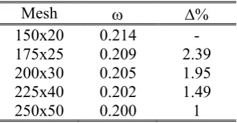
Mesh %
150x20 0.214 -
175x25 0.209 2.39 200x30 0.205 1.95 225x40 0.202 1.49
250x50 0.200 1
[image:9.595.206.379.88.178.2]
Table II: Outcomes of the grid refinement study (Pr=0.01, Ax=10, =0.1 and Gr = 4x10⁵).
As shown in Table II, the relative percentage error becomes smaller than 2% as the mesh density exceeds that corresponding to NxxNy=175x25. Accordingly, a mesh 200x30 has been used to
discretize the flow in the xy plane for all the cases treated in the present work. Following a common practice in the literature, for the 3D simulations we have scaled the number of points along the third (z) direction in a proportional way (i.e. 200 points along z when the extension in that direction is equal to the system size along x, leading to a total of 1.2x10⁶ nodes).
Obviously, an algorithm capable of targeting the broadest range of applications would also require assessment of the mesh resolution against typical criteria relating to the simulation of turbulent flows. For the sake of clarity, we delay the treatment of this specific point to Sect. 3.2 where we address it in conjunction with a description of chaotic convection and the typical related flow “scales” (in practice, the validity of the present approach has been further assessed by comparing the spatial grid spacing, in terms of x, y and z, with the so-called Kolmogorov length, that is the smallest, i.e. most demanding in terms of required numerical resolution, scale developed by the flow when turbulent conditions are established).
3. Results
A synthetic description of the salient outcomes of our numerical studies is reported in the remainder of this section (articulated in focused subsections) together with a critical discussion of some accompanying necessary concepts (provided to support reader’s understanding).
10
Most conveniently, first we address the case with the same value of the Prandtl number (i.e. Pr=0.01) already considered by Ref27 (in order to appreciate the differences, i.e. the new dynamics enabled by the third dimension), then we discuss in detail the effects produced by an increase in the Prandtl number.
3.1 Hydrodynamic and hydrothermal Disturbances
Following a deductive approach with systems of growing complexity being treated as the discussion progresses, we start from the trivial case in which the emerging flow is steady. As an example, for Pr=0.01, Az=10 and periodic boundary conditions with respect to the z direction, not surprisingly, at
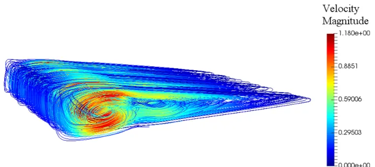
Ra=400 the flow pattern provided by the 3D simulations consists of a steady two-dimensional unicellular structure (not shown), which indicates that this relatively small value of the Rayleigh number is sufficient to excite neither hydrodynamic oscillatory disturbances, nor OLR modes. In agreement with Ref27, if the Rayleigh number is increased to 1000, a second circulation nucleates in the original unicellular structure (as shown in Fig. 2). This flow is still steady.
[image:10.595.112.482.375.540.2]When Ra is further increased, however, interesting departures from 2D behaviours occur. .
Figure 2: Streamlines of the steady base flow in different sections along the z direction for Pr=0.01
and Ra=1000, (Gr=105).
As a first example along this path, in particular, we examine the field obtained by doubling the Rayleigh number, i.e. Ra=2000.
11
a)
b)
[image:11.595.115.506.82.726.2]c)
Figure 3: Structure of 3D oscillatory flow for Pr=0.01, Az=10 (periodic boundary conditions),
12
Indeed, some peaks of velocity (red arrows) distributed along the spanwise direction (the z axis) can be recognised in this figure in proximity to the left side of the cavity (the thickest one), which undoubtedly prove the existence of a disturbance extending along this direction. The essentially 3D nature of the flow is also made evident by the presence of vortices in the entire xz plane.
Following up on the previous point, notably, these vortices do not undergo a progressive displacement (in time) along the positive or negative z direction (as one would expect for a travelling wave); rather they take part in an endless wandering process (moving back and forth about a position fixed in space resembling the behaviour of a standing wave).
Given the very small value of Pr relating to these phenomena (Pr=0.01) and the relatively low value of the Rayleigh number for which the oscillatory disturbances manifest themselves (a value smaller than that required to excite hydrodynamic disturbances in the equivalent 2D case), these simple observations implicitly define a conundrum, that is understanding whether these disturbances are of a hydrodynamic or hydrothermal (OLR) nature In such a quest, we exclude the presence of SLL modes like those reported in the study by Delgado-Buscalioni25, as though the walls of our cavity are inclined, the system is perfectly symmetric with respect to the horizontal direction (in other words, no net inclination is present as the opposite tilts of the top and bottom walls balance each other). Delgado-Buscalioni25 found stationary longitudinal rolls only in the presence of Rayleigh-Bénard modes excited in conjunction with inclinations able to produce a destabilising vertical component of the temperature gradient. In the present case this is not possible as the heated and cooled sides of the cavity remain always perfectly vertical, therefore no heating from below effect can be introduced due to wall inclination. Moreover, the vertical projection of the temperature stratification (eventually produced by the Hadley flow for relatively high values of Ra) is always opposite to gravity (leading to a heating-from-above effect).
Similarly, the occurrence of “Rayleigh” modes like those predicted in the linear stability by Gershuni et al.,37 for non-tilted layers with top and bottom conducting boundaries can also be filtered out. That kind of mode (yet emerging in the form of steady rolls with their axes aligned with the shear flow), indeed, follows from the presence of zones of potentially unstable stratification near the upper and lower horizontal boundaries induced by the basic flow, which are suppressed if the top and bottom walls are adiabatic (as in the present case).
Even with such initial simplifications, resolving the question formulated above about the nature of the present disturbances, however, is not straightforward as one would imagine as it requires separating different contributions, which are generally interwoven. Perhaps, the most obvious attempt to discern the underlying intricacies would be to start from the widespread existing consensus in the literature that for such systems some relevant considerations might be derived on the basis of simple “theorems” (which provide necessary and/or sufficient conditions for the onset of certain disturbances).
13
theorem, stating that: “In an inviscid shear flow a necessary condition for instability is that there must be a point of inflection in the velocity profile u=u(y),i.e. a point where d2u/dy2=0”. As illustrated by some author (Refs38-41), this condition also acts as a sufficient condition in many circumstances. Furthermore, the related disturbances are expected to be hydrodynamic in nature and purely two-dimensional (Squire42).
To some extent all these theorems apparently simplify the problem by abstracting some essential and distinctive features. Such arguments have often been used by several authors to support the conclusion that for small values of the Prandtl number the oscillatory disturbances found in two-dimensional numerical simulations of buoyancy flow in differentially heated rectangular cavities should be considered of a hydrodynamic origin (Refs36,43-48 and references therein).
The Squire’s theorem, however, is not applicable in the present case as the flow is not parallel (due to the opposing inclination of the top and bottom walls). Superimposed on this bottleneck, there are some drawbacks of conceptual nature. Since the Prandtl number is not exactly zero, technically speaking, the momentum and energy equations cannot be uncoupled, which also invalidates the outcomes of the Rayleigh theorem.
These initial reflections are instructive as they illustrate how any attempt to discern the origin of the perturbations shown in Fig. 3 on the basis of simple criteria or theoretical arguments should not be considered as a viable option.
Though some relevant information could be gathered by using the typical protocols of the linear stability analysis and related energy transport considerations, here we take a different approach potentially applicable also to situations in which the flow has rather a chaotic nature. More precisely, we show that direct numerical solution of the model equations in nonlinear form has still the potential to offer valuable insights provided it is critically used together with some physical reasoning about the different “natures” of the hydrodynamic and hydrothermal fundamental modes of instability.
Put simply, in order to shed some light on this issue, we apply the following strategy: additional simulations are performed uncoupling the energy and momentum equations (i.e. by assuming a fixed initial thermally diffusive distribution of temperature inside the entire physical domain and solving the balance equations for mass and momentum only).
The physical reasoning underlying this modus operandi is quite obvious. If the instability was thermal in nature (OLR mode), the oscillations would cease under such conditions because the temperature effects have been switched off; vice versa, they should survive if they were related to a hydrodynamic mode (owing to its purely shear-driven origin).
14
Figure 4: Projection of the velocity projection in the yz plane at x=1/8Ax (Pr=0.01, Az=10, periodic
boundary conditions, Ra=2000, temperature equation uncoupled).
As any processes that depend on the amplification of the aforementioned helicoidal disturbances are excluded in this case, these findings are of remarkable conceptual significance as they indicate that the main source of the oscillatory dynamics shown in Fig. 3 must therefore be ascribed primarily to a mechanism of hydrodynamic nature.
Accordingly, the following partial conclusions can be drawn for this specific case: Allowing the flow to extend along the third direction can cause a modification in the emerging dynamics with respect to those seen in the 2D case. The flow becomes oscillatory for a slightly smaller value of the Rayleigh number and display 3D features due to the presence of vortices in the xz plane (in addition to those generally seen in the xy plane). Despite these remarkable differences (with respect to that previously revealed by equivalent 2D studies), however, evidence points towards the conclusion that the fundamental nature of the most critical disturbance does not change (the spatio-temporal appearance is more complex, but the fundamental mechanisms driving the instability are essentially the same).
15
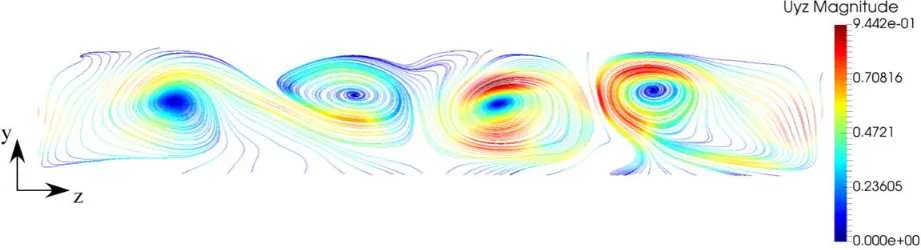
Figure 5: Isosurfaces (snapshot) of the w component of velocity (Pr=0.05, Az=10, periodic
boundary conditions, Ra=2000, Gr=4x10⁴, OLR mode).
For Pr=0.05 and the same conditions considered in Fig. 3 (periodic boundary conditions, Az=10 and
Ra=2000), the intricate behaviour seen for Pr=0.01 is replaced by a much more periodic and regular pattern.
As evident in Fig. 5, another distinguishing mark of this emerging mode is its spatial configuration, the oscillatory behaviour being confined to the part of the cavity with the larger vertical extension, with a quasi-steady state attained in the narrower region.
Figure 6: Oscillatory convection (Pr=0.05, Az=10, periodic boundary conditions, Ra=2000,
Gr=4x10⁴): four snapshots of non-dimensional velocity magnitude in the xz plane evenly distributed in space (OLR with nondimensional angular frequency 2.81).
[image:15.595.81.540.441.566.2]16
Figure 7: Four snapshots of non-dimensional velocity magnitude for the same conditions
considered in Fig. 6.
Following the same approach undertaken for Pr=0.01, towards the end to clarify the nature of this disturbance, we have repeated such simulation switching off the solution of the temperature equation (yet to filter out any disturbance of thermal buoyancy nature).
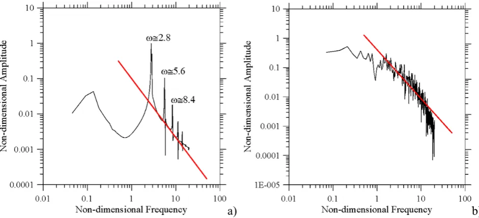
The outcomes of this study are summarised in Figs. 8 and 9, where we have reported the spectrum of frequencies for the different situations examined so far, namely Pr=0.01 with coupling between the energy equation and the Navier-Stokes equations enabled and disabled (Fig. 8a and 8b, respectively) and the analogous spectra for the case with Pr=0.05 (Figs. 9a and 9b, respectively, the reader being referred to the next section for additional discussions).
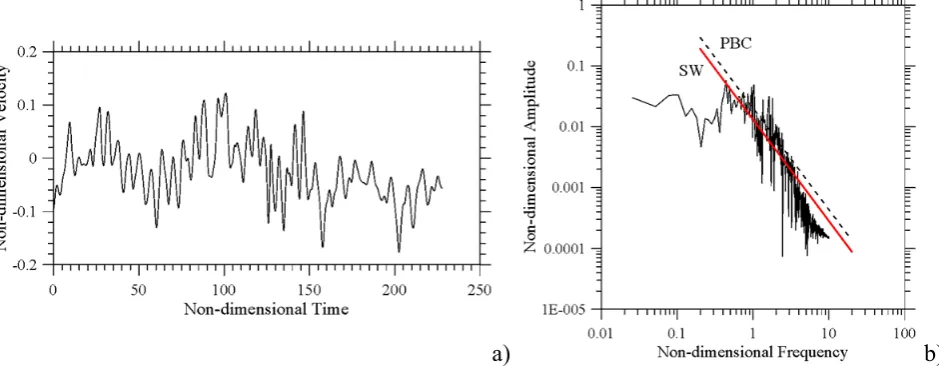
3.2 Frequency spectra and multiple solutions
By simple visual inspection of the frequency spectrum, it is evident that it is rather chaotic for Pr=0.01 (Fig. 8a corresponds to the disordered pattern shown in Fig. 3), whereas only one frequency (and its multiples) can be seen in Fig. 9a (corresponding to Fig. 5).
Additional insights follow naturally from the corresponding plots obtained by uncoupling the momentum and energy equations.
17
[image:17.595.63.531.69.282.2]a) b)
Figure 8: Frequency spectra (Pr=0.01, Az=10, periodic boundary conditions, Ra=2000, Gr=2x10⁵):
a) temperature equation coupled (mixed regime with dominant hydrodynamic modes and OLR with 0.6), b) temperature equation uncoupled (purely hydrodynamic oscillatory mode of convection).
a) b)
Figure 9: Frequency spectra (Pr=0.05, Az=10, periodic boundary conditions, Ra=2000, Gr=4x10⁴):
a) temperature equation coupled (OLR mode), b) temperature equation uncoupled (hydrodynamic oscillatory mode of convection).
[image:17.595.61.532.364.578.2]18
so surprising if one considers that the neutral curves predicted by the linear stability analyses for these two fundamental modes of convection in infinite layers are relatively close. As an example, in the case of horizontal layers, Hart16 found the hydrodynamic disturbances to be the most dangerous for Pr<0.015, this role being taken over by the OLR mode in the range 0.015<Pr<0.27. Kuo and Korpela44 confirmed and slightly revised these results showing that for Prandtl number less than 0.033, the shear disturbances are the dominant instability mechanism, whereas the instability is triggered in the form of oscillating longitudinal rolls in the range 0.033<Pr<0.2 (the critical curves for these two different categories of disturbances were yet found to be relatively close one to another in terms of values of the Rayleigh number). Similarly, Delgado-Buscalioni25 reported a codimension-two point located approximately at Pr0.03 for purely horizontal cavities, moving towards smaller values of Pr for slightly inclined configurations.
Though the coexistence of different instability modes might have been anticipated on the basis of the information provided by linear stability analyses, the most unexpected aspect revealed by the present simulations is the rather turbulent nature of the flow emerging for small values of the Rayleigh number when the dominant disturbances are hydrodynamic in nature (Figs. 8a, 8b and 9b). In equivalent 2D simulations27, the flow was found to be laminar. As an example, for Ra = 9000 (see Fig. 11 Ref27), a bimodal state with two incommensurate frequencies was obtained. As shown here (Fig. 8), the 3D flow is featured by a much more complex multimodal temporal behaviour even if the Rayleigh number is as small as 2000. Even more interestingly, this flow displays the ability to develop a range of scales where the energy power spectrum satisfies the well-known scaling law predicted by Kolmogorov49-52 (represented by the inclined red line in Fig. 8).
In order to emphasize this specific aspect, we have used the same approach illustrated by De et al.,53, i.e. we have reported the frequency and related amplitude using logarithmic scales for the axes and comparing the resulting diagram with a power law P() = (/c)−s (where c is a fitting parameter).
Such a comparison has provided evidence that the frequency spectrum of velocities aligns perfectly with an −5/3 law in a wide band of frequencies, as implicit in the so-called turbulence similarity
hypothesis.
19
Interestingly, this feature is retained if the periodic boundary conditions at z=0 and z=Az=10 are
replaced by adiabatic solid walls (see Fig. 10), which indicates the hydrodynamic disturbances, responsible for the cascade of energy from large scales towards smaller ones, have all nondimensional wavelength in the range between zero and Az.
[image:19.595.65.535.164.347.2]a) b)
Figure 10: Numerical simulation for Pr=0.01, Az=10, solid walls along the z direction, Ra=2000
(Gr=2x10⁵): a) Velocity signals at a fixed point (x=3/8Ax, y=0, z=Ax/2), b) frequency spectrum.
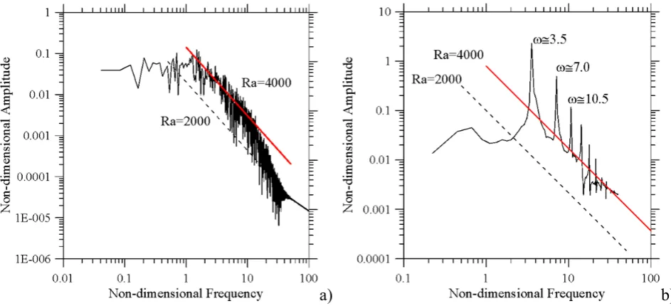
To put our results in a broader context, we have allowed the Rayleigh number to grow further. Results for Pr=0.01 and Ra=4000 can be seen in Figs. 11a and 12a. The major outcome is that, while for this value of the Rayleigh number the emerging state under the constraint of two-dimensionality would correspond to a simple periodic (single-frequency) wave travelling in the streamwise direction25, the 3D results yet demonstrate the existence of an extended set of scales through which the energy is transferred from larger to smaller eddies (slightly shifted to the right of the plot with respect to the corresponding interval seen in Fig. 8a). Making Ra higher, as expected, also produces an increase in the energy content of the flow (as witnessed by the upward shift of the straight line representing the aforementioned 5/3 law).
Apart from the differences between 2D and 3D results, the present findings are relatively surprising if one also considers that in other “similar” problems (buoyancy convection in heated systems for fluids with Prandtl number Pr O(1) and values of Gr=O(105) or O(106)), in general, the two just mentioned scales limiting the cascade from below and from above differ by several (3 or more) orders of magnitude53,54.
20
instability), on the other hand the extension of the inertial range is relatively limited (covering just a limited set of scales as shown in Figs. 8a, 8b and 9b and 10).
[image:20.595.60.532.123.338.2]a) b)
Figure 11: Frequency spectra: a) Pr=0.01, Az=10, periodic boundary conditions, Ra=4000,
Gr=4x10⁵ (regime with dominant hydrodynamic modes), b) Pr=0.05, Az=10, periodic boundary
conditions, Ra=4000, Gr=8x10⁴ (OLR mode: though for this case the scaling seems to be compatible with the Kolmogorov law, this regime cannot be considered a turbulent one as the spectrum displays just a fundamental frequency and its high-order multiples).
a) b)
Figure 12: Isosurfaces (snapshot) of the w component of velocity for the same conditions
considered in Fig. 11a and 11b, respectively.
[image:20.595.61.534.449.590.2]21
In general, Figs 12a and 12b may be regarded as a natural continuation of Figs. 3 and Fig. 5, respectively.
Under a slightly different perspective, these simple observations might be used to conclude that while the flow is allowed to enter the so-called inertial regime at low Ra when hydrodynamic disturbances are spontaneously selected by the system (most critical disturbances), or artificially induced (preventing the system from “selecting” OLR modes), the attainment of this regime is delayed to larger values of the Rayleigh number when the OLR perturbations are preferred.
Following this very interesting argument and taking into account that Gr=Ra/Pr represents directly the ratio of buoyant to molecular viscous transport, we deemed it necessary to compare the response of the two different fluids for the same value of the Grashof number (as Gr measures the relative importance of the driving force with respect to the opposing viscous effects, it can be regarded as an analogue of the Reynolds number generally used in the literature as a universal “control” parameter in studies about the onset of turbulence).
In line with the expected outcomes, Fig. 13 shows that for Gr=2x10⁵, for both values of Pr conditions are established for which the inertial regime can develop (compare, e.g., Figs. 8a and 13a).
[image:21.595.73.521.377.570.2]a) b)
Figure 13: Properties of oscillatory convection for Pr=0.05, Az=10, periodic boundary conditions,
Ra=10000 (Gr=2x10⁵, mixed regime with hydrodynamic and OLR modes): a) frequency spectrum, b) isosurfaces (snapshot) of the w component of velocity.
22
in Fig.12b and Fig. 3) and 2) enhance the turbulent nature of the emerging flow by making the spectra more involved.
Following up on the observation above, we conclude the present section by highlighting the interesting affinity between the present findings and some earlier results presented by Delgado-Buscalioni et al.,55.
These authors performed 3D numerical calculations of natural convection for Pr=0.025 in an enclosure with Ax=4 and Az=6 inclined at 10° with respect to the horizontal direction (such a case
being considered due to the expected coexistence of transversal and longitudinal instabilities given the location of the aforementioned codimension-two point at Pr0.03). For the sake of comparison between 3D and 2D results, they also examined the corresponding 2D enclosure (allowing (purely twodimensional oscillatory hydrodynamic modes only to develop).
Under the constraint of two-dimensionality, a first bifurcation to oscillatory flow was identified, followed on increasing the Rayleigh number by a period-doubling bifurcation. When the constraint of 2D flow was removed, the initial two-dimensional stationary convection was found to undergo a Hopf bifurcation at values of Ra lower than the corresponding ones for the 2D case, with the flow breaking due to the onset of an oscillatory convection with three longitudinal rolls. A secondary frequency for the 3D flow, observed at Gr5x105, was found to be basically related to the formation of a bicellular transversal pattern giving rise to a mixed regime with hydrodynamic and OLR modes resembling the dynamics described in the present section (namely, the visible enhancement of turbulence where more instabilities can easily interact).
3.3 Kolmogorov scales and multiple solutions
Additional insights into the dynamics presented in the earlier sections follow naturally from direct comparison with estimates available in the literature about the time scale limiting the inertial range from below, i.e. the so-called Kolmogorov time scale (t). Following Paolucci56,Farhangnia et al.,57,
in a transversely heated cavity, the Kolmogorov time and length scales can be evaluated, respectively, as:
3
1/4 8 Prt Ra
(5)
3/8 16 Pr
s
Ra
(6)
23
Pr Gr Ra t s
0.01 2x10⁵ 2000 0.266 0.091
0.01 4x10⁵ 4000 0.158 0.070
0.05 4x10⁴ 2000 0.178 0.167
0.05 8x10⁴ 4000 0.106 0.129
0.05 2x10⁵ 10000 0.053 0.091
0.05 4x10⁵ 20000 0.032 0.07
Table III: Kolmogorov length and time scales as a function of the Prandtl, Grashof and Rayleigh
numbers.
By comparing Table III with the spectra shown in Figs. 8a and 11a for Pr=0.01, the reader will realise that the shift to the right of the inertial regime produced by an increase in the value of the Rayleigh number is in agreement with the corresponding decrease in the Kolmogorov time scale predicted by eq. (5) (by indicating with max the recognisable maximum value taken by the angular
frequency of the disturbance at the end of the inertial regime in these two figures, it can easily be verified that the following correlation holds: max 2/t). Such a relationship, however, is no
longer valid for the cases with Pr=0.05 and Ra=2000 or 4000 and the only key to understanding such results lies in considering that the related flow has not entered yet the inertial regime (2/t >>max).
Nevertheless, the agreement between max and the corresponding Kolmogorov frequency for
Pr=0.05 holds for Ra=10000 (Gr=2x10⁵), which confirms the expectation (as already discussed to a certain extent in the preceding text) that the Grashof number should be considered as a more relevant parameter in comparative studies of the process leading liquid metals in differentially heated cavities to develop turbulence (for Gr=2x10⁵ and both values of Pr, the frequency spectra display the typical features of this regime, Figs. 8a and 13a).
[image:23.595.69.521.527.713.2]b) b)
Figure 14: Properties of oscillatory convection for Pr=0.05, Az=10, periodic boundary conditions,
24
Nature, however, does not always follow apparently logical rules or “straightforward” (obvious) evolution paths, especially when highly non-linear systems are considered. Most unexpectedly (see Fig. 14a), the agreement with the predicted Kolmogorov frequency ceases and the typical features of the inertial regime are no longer there as the Grashof number grows further. For Gr=4x10⁵, indeed, the frequencies visible in the spectrum take again the same scattered appearance already reported for smaller values of Gr. Along these lines, the reader may compare directly Fig. 14a with the corresponding spectrum shown in Fig. 11b for Gr=8x10⁴; apart from the expected increase in the main frequency (maximum visible peak) and ensuing displacement of the other harmonics to the right, these spectra are very similar; comparison of the isosurfaces in Figs. 14b and 13b also leads to the conclusion that on increasing Gr, the flow takes a more spatially regular structure resembling that of classical OLR disturbances.
25
[image:25.595.66.529.75.267.2]a) b)
Figure 15: Properties of oscillatory convection (mixed regime with hydrothermal and
hydrodynamic modes) for Pr=0.05, Az=10, periodic boundary conditions, Ra=20000 (Gr=4x10⁵),
initial conditions corresponding to Fig. 13b: a) frequency spectrum, b) isosurfaces (snapshot) of the w component of velocity.
The results, summarised in Fig. 15, definitely confirm that the multiplicity of solutions is indeed a feature of the considered problem as the velocity field produced in this way retains the same “turbulent” features seen in Fig. 13. The discrete frequency spectrum reported in Fig. 14a is taken over by a distribution where the amplitude of oscillations varies continuously with over an extended interval (to fix ideas, we can think of the state shown in Fig. 15 as a “continuation” of that reported in Fig. 13, existing in parallel with that in Fig. 14).
This interesting result also sheds some additional light on our earlier finding (the main outcomes being shown in Fig. 9) about the possibility to replace a state dominated by OLR with a new solution in which hydrodynamic disturbances become pervasive by uncoupling the momentum and energy balance equations. Besides the canonical method based on a variation of the basin of attraction, the inhibition of temperature disturbances by equations uncoupling should indeed be seen as another possible way to drive the system along a given path of evolution in the case of coexisting “attractors”. Obviously, while with the approach based on a variation of the initial conditions it is not possible to predict in which “direction” the system will evolve, by disabling the energy equation the system if forced to select and amplify hydrodynamic disturbances, these being the only allowed ones when the temperature does not play an active role in the instability mechanism.
Notably, the agreement with the data reported in Table III is back when the end of the spectrum in Fig. 15a is considered.
26
Kolmogorov length. For the present case, by indicating with x, y and z the space integration steps along the three fundamental directions of the Cartesian coordinate system, the reader will easily realise that the above criterion is largely met with s / x, s / y and s / z, all being 1 for
all the values of Gr reported in this table.
[image:26.595.59.533.159.373.2]a) b)
Figure 16: Frequency spectra for the cases with solid walls delimiting the system along the z
direction (Pr=0.01, Ra=4000, Gr=4x10⁵): a) Az=2, b) Az=5.
Taken together Figs 16 and 17 finally show that the presence of limiting walls perpendicular to z can have an appreciable impact on the properties of the inertial regime by causing, on the one hand, a decrease in the number of modes (due to the suppression of all disturbances with wavelength larger than Az=10) and, on the other hand, an ensuing mitigation of the energy content.
27
[image:27.595.144.452.81.226.2]b)
Figure 17: Isosurfaces (snapshot) of the w component of velocity for the same conditions
considered in Fig. 16a and 16b, respectively.
As a concluding remark, we would like to point out the following: All the information reported in this section are valuable on their own due to the insights they give into the high-dimensional chaotic state of these flows in terms of involved time and length scales (and their scaling with the problem characteristic numbers). Unfortunately, however, they cannot be used to provide clues or hints about the “process” leading the flow to enter this regime. In other words, targeting an improved understanding of the mechanisms by which a number of coexisting modes can be developed when the main problem parameter (the Rayleigh number or the Grashof number in our case) is progressively increased is not possible in this framework.
The reader is referred to the next section for further elaboration of these aspects, the introduction of adequate concepts and related applications/implications.
3.4 Correlation dimension and transition from low-dimensional to high-dimensional chaos
For the purpose of quantifying the rate of increase of the degrees of freedom of the system, in practice, one has to evaluate the so-called fractal or “correlation” dimension for different situations. Such a strategy obviously requires some justification and theoretical reasoning. Perhaps, the best way to introduce the related discussion is to start from the remark that the dynamics of a chaotic system can generally be connected to its dimension in a “relevant space”.
28
definition can be introduced to characterise the dimensionality of an “object”. In particular, the need for new definitions specifically applies to the items which represent “attractors”, i.e. subsets of the space of phases such that different trajectories arising from different points of the subset end on the subset anyway.
[image:28.595.153.445.286.568.2]For such objects, the notion of dimension can properly be extended to account for other features, one of these being the rate with which a typical orbit “visits” different parts of the attractor (let us shortly recall that the evolution of a dynamical system can always be described by means of an “orbit”, which is a curve traced in the phase space having as many dimensions as the number of degrees of freedom of the system). In particular, this feature can naturally be incorporated into the concept of natural measure, namely the percentage of the time that an orbit takes for any given region of the space.
Figure 18: Correlation Dimension as a function of the Rayleigh number (Pr=0.01, Az=10, periodic
boundary conditions).
This quantity can be estimated by taking the following limit (provided it exists):
) , , ( lim ) ,
(C z C zo t t
o
(7)
where C is the generic cube in the phase space, z(zo,t) is the orbit originating from a generic initial
condition zo, and (C,zo,t) formally represents the percentage of time that z(zo,t) spends in C in a
29
naturally paves the way to that of fractal object and correlation dimension. Assuming the phase space to be partitioned via an r-grid, the latter can formally be introduced (Balatoni and Renyi55) as:
) ln( ) ( ln lim 1 2 02
r C j j r D (8)
This dimension, which by definition is “a measure of the dimensionality of the space occupied by a set of random points” (Grassberger61) is generally regarded as an effective measure of the number of “active modes” in a dynamical system, or of the "number of degrees of freedom” (Theiler62). Over the years, algorithms able to yield an estimate of this quantity have been elaborated, a relevant example being represented by the original work by Grassberger and Procaccia63,64. The values taken by D2 for the conditions considered in the present work are summarised in Fig. 18. By embodying the concept of progressively increasing structure on finer and finer length scales, and the related concept of sensitivity to the initial conditions, the growing non-integer values displayed by D2 clearly reveal the emergence of features typical of chaos.
Interestingly, as soon as Ra exceeds 1550, D2 becomes larger than 3 (D23.14 for Ra=1550, D2 4.22 for Ra=1580) and then suddenly grows for higher values of Ra. Such a gain in chaotic features can clearly be interpreted as the quick development of fully developed turbulence (as witnessed by the number of coexisting modes visible in the final state shown in Fig. 8a for Ra=2000; the reader being also referred to the sequence of signals reported in Fig. 19 for increasing values of Ra).
30
a)
b)
c)
[image:30.595.117.483.76.619.2]d)
Figure 19: Velocity signals at a fixed point (x=3/8Ax, y=0, z=Ax/2) for Pr=0.01, Az=10, periodic
boundary conditions and different values of the Rayleigh number: a) Ra=1400, b) Ra=1550, c) Ra=1700, d) Ra=2000.
31
For the simple case of only two incommensurate frequencies the phase trajectory may be imagined as a set of points pertaining to a toroidal surface T2 in the three-dimensional phase space. According to the classical Ruelle-and-Takens scenario a third independent frequency should always appear before transition to chaos is permitted, i.e. the attractor should become a hypertorus T3. This is indeed what is formalised by the so-called Newhouse-Ruelle-Takens theorem (Newhouse et al.,67), which asserts that a torus T3, under the actions of some perturbations, degenerates to a "strange attractor", and therefore the existence of three frequencies (i.e. three degrees of freedom) should generally be regarded as a necessary and sufficient condition for the onset of a chaotic regime. The indirect outcome of our observations in the present case is that, by allowing transition to chaos directly from a torus T2, the present findings are another example of results supporting the alternate route towards chaos proposed by Curry and Yorke68. These authors theorised direct transition to chaos via gradual deformation of an initially closed curve in the phase space due to a continuous stretching and folding process (the reader being referred to the work by Paul et al.,69 and reference therein about other related examples in the literature, e.g., the Curry-Yorke scenario in Rayleigh-Bénard convection).
4. Conclusions
Continuing an earlier work where the analysis of the problem related to the Hadley circulation in containers with non-horizontal top and bottom walls and no net inclination was limited to purely two-dimensional flow (chosen as an archetypal situation where the well-known Squire and Rayleigh criteria are no longer valid), in the present analysis we have explored the 3D effects that emerge when the constraint of two-dimensionality is removed.
In the literature often a dichotomy has been drawn between the two fundamental categories of fluid-dynamic disturbances thought to be enabled in such circumstances, namely, two-dimensional hydrodynamic and hydrothermal (helicoidal) modes. We have shown that these two models (transverse and longitudinal rolls) are opposite idealised extremes, both being severe approximations to a more complete representation of reality. In particular, we have been found that these disturbances are not mutually exclusive, nor are they progressive and that the development of turbulence via a hierarchy of instabilities can involve a rich variety of concurrent paths or lines of evolution.
The subject has been addressed via numerical solution of the overarching set of equations, including the mass, momentum and (internal) energy balance laws. These equations have been solved numerically in their complete, non-linear, time-dependent and fully coupled form.
A variegated strategy of attack has been implemented to address such a complex subject, including (but not limited to) an analysis of the ability of these systems to develop multiple branches of solution and related progression from low-dimensional to high-dimensional chaos.
32
assuming canonical initial conditions corresponding to a thermally diffusive quiescent state or using already developed flow at a given value of the Rayleigh number as initial state to explore the effects produced by an increase in such parameter.
As such strategy, however, cannot produce clues about the connections between the initial state and the nature of the emerging disturbance, in parallel, further understanding of these instabilities has been gained by uncoupling the momentum and energy equations (a fruitful alternative for obtaining insights that are hidden to experimental analysis and which allows new paths of enquiry to be proposed). Both these approaches provided independent lines of evidence pointing towards the same conclusion, namely, that for this problem multiple states exist which can replace each other in given sub-regions of the space of parameters.
In particular, for the smallest considered values of the Prandtl number (Pr=0.01), the emerging disturbances have been found to cause sudden transition to relatively chaotic states for values of the Rayleigh number even smaller than those required to excite regular (time-periodic) waves travelling in the streamwise direction in the 2D case. These perturbations clearly display a 3D nature as witnessed by the presence of recognisable velocity peaks along the third direction and spatially extended vortices in the xz plane. Equation uncoupling (in the framework of the approach described above) has been instrumental in discerning that temperature variations and related buoyancy effect play no role in the mechanisms leading to the amplification of such (hydrodynamics) perturbations and ensuing sudden transition to chaos.
On the other hand, fully coupled simulations have demonstrated that the spatially pervasive presence of hydrodynamics modes does not prevent the system from developing in parallel OLR flow, as witnessed by the presence of specific recognisable peaks in the frequency spectrum (these peaks are no longer visible inasmuch the OLR is no longer allowed to exist without temperature and momentum coupling).
Though these OLR modes tend to be more frequent as the Prandtl number is increased and their emergence seems to rule out the development of hydrodynamic disturbances (at least for relatively small values of the Rayleigh number), however, hydrodynamic modes overwhelmingly re-enter the dynamics as soon as the momentum and energy balance equations are uncoupled or the Grashof number is sufficiently increased.
33
(for the same value of the Grashof number) with the turbulent ones discussed above in the form of “multiple solutions”.
Regardless of the considered Prandtl number, in general, higher values of the Grashof number have been found to produce a two-fold effect, i.e. an increase in the average energy content of the flow and an expansion of the “extension” (in terms of involved scales) of the inertial range.
Additional insights into the onset of this kind of turbulence have been obtained through evaluation of the so-called correlation dimension for conditions in which the chaos can still be considered low-dimensional (relatively small values of Ra or Gr). Through this quantity (generally used to characterise the “fractal nature” of “attractors” in the space of phases), we could track precisely the progression of the system from an initial quasi-periodic state towards fully developed turbulence due to the progressive excitation of new “degrees of freedom”. By virtue of this approach, in particular, we could discern that the transition from low-dimensional to high-dimensional chaos takes a specific path, which falls under the general heading of Curry-Yorke scenario (that is direct transition to chaos being allowed via gradual corrugation of a T2 torus).
References
[1] Okano Y., Itoh M. and Hirata A., (1989), Natural and Marangoni Convections in a Two-Dimensional Rectangular Open Boat, Journal of Chemical Engineering, 22(3), 275-281.
[2] Delgado-Buscalioni R. and Crespo del Arco E., (2001), Flow and heat transfer regimes in inclined differentially heated cavities, Int. J. Heat Mass Transfer, 44, 1947-1962.
[3] Kaddeche S., Henry D. and Ben Hadid H., (2003), Magnetic stabilization of the buoyant convection between infinite horizontal walls with a horizontal temperature gradient, J. Fluid Mech., 480, 185-216.
[4] Li Y.R., Peng L., Wu S.-Y., Imaishi N., Zeng D.L., (2004), Thermocapillary-buoyancy flow of silicon melt in a shallow annular pool, Cryst. Res. Tech, 39(12), 1055-1062.
[5] Jaber T.J. and Saghir M.Z., (2006), The Effect of Rotating Magnetic Fields on the Growth of SiGe Using the Traveling Solvent Method, Fluid Dyn. Mater. Process., 2(3), 175-190.
[6] Lappa M., Thermal Convection: Patterns, Evolution and Stability, John Wiley & Sons, Ltd (2009, Chichester, England).
[7] Ludwig A., Gruber-Pretzler M., Wu M., Kuhn A. and Riedle J., (2005), About the Formation of Macrosegregations During Continuous Casting of Sn-Bronze, Fluid Dyn. Mater. Process., 1(4), 285-300.
[8] Abhilash E., Joseph M.A. and Krishna P., (2006), Prediction of Dendritic Parameters and Macro Hardness Variation in Permanent Mould Casting of Al-12%Si Alloys Using Artificial Neural Networks, Fluid Dyn. Mater. Process., 2(3), 211-220.
34
[10] Dupret F. and Van der Bogaert N., Modelling Bridgman and Czochralski growth, in Handbook of Crystal Growth (ed. D. T. J. Hurle) 2: 877-1010. North-Holland, Amsterdam (1994).
[11] Monberg E., “Bridgman and related growth techniques”. In Handbook of Crystal Growth (ed. D. T. J. Hurle), 2: 53-97. North-Holland, Amsterdam (1994).
[12] Zrodnikov A.V., Efanov A.D., Orlov Yu.I., Martinov P.N., Troynov V.M., Rusanov A.E., (2004), Technology of heavy liquid metal coolants lead-bismuth and lead, VANT, Serial: Provision of NPP Safety, Issue 4, Nuclear Technologies for Future Power System, 180-184.
[13] Gorse-PomontiD., and Russier V., (2007), Liquid metals for nuclear applications, Journal of Non-Crystalline Solids, 353(32–40), 3600-3614.
[14] Luo M. and Liu J., (2013), Experimental investigation of liquid metal alloy based mini-channel heat exchanger for high power electronic devices, Frontiers in Energy, 7(4), 479-486. DOI: 10.1007/s11708-013-0277-3
[15] Hart J.E., (1972), Stability of thin non-rotating Hadley circulations,. J. Atmos. Sci., 29, 687-697. [16] Hart J.E., (1983), A note on the stability of low-Prandtl-number Hadley circulations, J. Fluid Mech., 132, 271-281.
[17] Gill A. E., (1974), A theory of thermal oscillations in liquid metals, J. Fluid Mech. 64 (3), 577-588.
[18] Afrid M. and Zebib A., (1990), Oscillatory three-dimensional convection in rectangular cavities and enclosures, Phys. Fluids, 2(8), 1318-1327.
[19] Hung M. C. and Andereck C. D., (1988), Transitions in convection driven by a horizontal temperature gradient, Physics Letters A 132(5), 253-258.
[21] Pratte J. M. and Hart J. E., (1990), Endwall driven, low Prandtl number convection in a shallow rectangular cavity, J. Cryst. Growth, 102, 54-68.
[22] Braunsfurth M. G. and Mullin T., (1996), An experimental study of oscillatory convection in liquid gallium, J. Fluid Mech., 327, 199-219.
[23] Wakitani S., (2001), Numerical study of three-dimensional oscillatory natural convection at low Prandtl number in rectangular enclosures, J. Heat Transfer, 123, 77-83.
[24] Hadley G., (1735), Concerning the cause of the general trade winds, Phil. Trans. Roy. Soc. Lond., 29, 58-62.
[25] Delgado-Buscalioni R., (2001), Convection patterns in end-heated inclined enclosures, Phys. Rev. E 64, 016303 (17 pages).
[26] Delgado-Buscalioni R., (2002), Effects of thermal boundary conditions and cavity tilt on hydrothermal waves: Suppression of oscillations, Phys. Rev. E, 66, 016301 (14 pages).
[27] Lappa M. and Ferialdi H., (2017a), On the Oscillatory Hydrodynamic Instability of Gravitational Thermal Flows of Liquid Metals in Variable Cross-section Containers, Phys. Fluids, 29(6), 064106 (19 pages).
35
[30] Yen R.H. and Liu C.H., (1993), Enhancement of the SIMPLE algorithm by an additional explicit corrector step, Numer Heat Transfer, Part B, 24, 127–141.
[31] Moukalled F., Mangani L. and Darwish M., (2016), The Finite Volume Method in Computational Fluid Dynamics - An Advanced Introduction with OpenFOAM and Matlab, Springer International Publishing, 2016, New York).
[32] Ladyzhenskaya O.A., (1969), The Mathematical Theory of Viscous Incompressible Flow, Gordon and Breach, 2nd Edition, New York - London, 1969.
[33] Choi SK, Nam HY, Cho M (1994) Systematic comparison of finite-volume calculation methods with staggered and nonstaggered grid arrangements, Numer Heat Transfer, Part B 25 (2), 205–221
[34] Choi SK, Nam HY, Cho M (1994a) Use of staggered and nonstaggered grid arrangements for incompressible flow calculations on nonorthogonal grids, Numer Heat Transfer, Part B 25(2), 193– 204.
[35] Rhie C.M. and Chow W.L., (1983), Numerical study of the turbulent flow past an airfoil with trailing edge separation, AIAA J 21,1525–1532
[36] Gelfgat A.Yu., Bar-Yoseph P.Z. and Yarin A.L., (1999), Stability of Multiple Steady States of Convection in Laterally Heated Cavities, J. Fluid Mech., 388, 315-334.
[37] Gershuni G.Z., Laure P., Myznikov V.M., Roux B., Zhukhovitsky E.M., (1992), On the stability of plane-parallel advective flows in long horizontal layers, Microgravity Q., 2(3): 141-151. [38] Tollmien W., (1936), General instability criterion of laminar velocity distributions, Tech. Memor. Nat. Adv. Comm. Aero., Wash. No. 792 (1936).
[39] Lin C.-C., (1944), On the stability of two-dimensional parallel flows, Proc. NAS, 30(10), 316-324.
[40] Rosenbluth M.N. and Simon A., (1964), Necessary and sufficient conditions for the stability of plane parallel inviscid flow, Phys. Fluids, 7(4), 557-558.
[41] Drazin P. and Howard L.N., (1966), Hydrodynamic stability of parallel flow of inviscid fluid, Adv. Appl. Mech., 9, 1-89.
[42] Squire H.B., (1933), On the stability of three-dimensional disturbances of viscous flow between parallel walls, Proc. R. Soc. London, Ser. A, 142, 621-628.
[43] Laure P. and Roux B., (1989), Linear and non linear study of the Hadley circulation in the case of infinite cavity, J. Cryst. Growth, 97(1), 226-234.
[44] Kuo H. P. and Korpela S. A. (1988), Stability and finite amplitude natural convection in a shallow cavity with insulated top and bottom and heated from the side, Phys. Fluids, 31, 33–42. [45] Wang T.-M. and Korpela S.A., (1989), Longitudinal Rolls in a Shallow Cavity Heated from a Side, Phys. Fluids A, 32, 947-953.
[46] Crespo del Arco E., Pulicani P. P., and Randriamampianina A., (1989), Complex multiple solutions and hysteresis cycles near the onset of oscillatory convection in a Pr = 0 liquid submitted to a horizontal temperature gradient, C. R. Acad. Sci. Paris, II 309, 1869-1876.
36
[48] Okada K. and Ozoe H., (1993), The Effect of Aspect ratio on The critical Grashof number for Oscillatory Natural Convection of Zero Prandtl Number Fluid: Numerical Approach, J. Cryst. Growth, 126, 330-334.
[49] Kolmogorov, A.N. (1941a) The local structure of turbulence in incompressible viscous fluids at very large Reynolds numbers, Dokl. Akad. Nauk. SSSR 30, 299-303. Reprinted in Proc. R. Soc. London A 434, 9-13 (1991).
[50] Kolmogorov, A.N. (1941b) On the degeneration of isotropic turbulence in an incompressible viscous fluids, Dokl. Akad. Nauk. SSSR 31, 538-541.
[51] Kolmogorov, A.N. (1941c) Dissipation of energy in isotropic turbulence. Dokl. Akad. Nauk. SSSR, 32, 19-21.
[52] Kolmogorov, A.N. (1942) Equations of turbulent motion in an incompressible fluid. Izv. Akad. Nauk. SSSR ser. Fiz. 6, 56-58.
[53] De A.K., Eswaran V., Mishra P.K., (2017), Scalings of heat transport and energy spectra of turbulent Rayleigh-Bénard convection in a large-aspect-ratio box, Int. J. Heat Fluid Flow, 67, 111– 124.
[54] Lappa M. and Gradinscak T., (2018), On the Oscillatory Modes of Compressible Thermal Convection in inclined differentially heated cavities, Int. J. of Heat and Mass, 121, 412–436.
[55] Delgado-Buscalioni R., Crespo del Arco E. And Bontoux P., (2001), Flow transitions of a low-Prandtl-number fluid in an inclined 3D cavity, Eur. J. Mech. B/Fluids, 329: 1-17.
[56] Paolucci S., (1990), Direct numerical simulation of two-dimensional turbulent natural convection in an enclosed cavity, J. Fluid Mech., 215, 229-262.
[57] Farhangnia M., Biringen S, Peltier L. J., (1996), Numerical Simulation of Two-dimensional Buoyancy-driven Turbulence in a Tall Rectangular Cavity, Int. J. Numer. Meth. Fluids, 23(12), 1311 - 1326.
[58] Shishkina O., Stevens R.J.A.M., Grossmann S. and Lohse D., (2010), Boundary layer structure in turbulent thermal convection and its consequences for the required numerical resolution, New J. Phys. 12, 075022 (17 pages).
[59] Bergè P., Pomeau Y., and Vidal C., (1984), Order Within Chaos-Towards a Deterministic Approach to Turbulence, John Wiley, New York, 1984.
[60] Balatoni J. and Renyi A., (1956), Publ. Math. Inst. Hung. Acad. Sci. 1, 9 (in Hungarian) [translation: Selected papers of A. Renyi, Vol. 1 (Budapest Academy, 1976) p. 558].
[61] Grassberger P., (1983), Generalized dimensions of strange attractors, Physics Letters A, 97(6, 5), 227-230.
[62] Theiler J., (1986), Spurious dimension from correlation algorithms applied to limited time-series data, Physical Review A, 34(3), 2427-2432.
[63] Grassberger P. and Procaccia I., (1983a), Characterization of Strange Attractors, Phys. Rev. Lett., 50, 346-349.
[64] Grassberger P. and Procaccia I., (1983b), Measuring the strangeness of strange attractors, Physica D, 9, 189-208.
37
[66] Eckmann J. -P. and Ruelle D., (1991), Fundamental Limitations for Estimating Dimension and Liapunov Exponents in Dynamical Systems, Physica D: Nonlinear Phenomena, 56(2-3), 1-4.
[67] Newhouse S., Ruelle D. and Takens T., (1978), Occurrence of Strange Axiom-A Attractors Near Quasi-Periodic Flows on Tm, m3, Commun. Math. Phys., 64: 35-40.
[68] Curry J and Yorke J.A., (1977), A transition from Hopf bifurcation to chaos: computer experiments with maps R2, in The structure of attractors in dynamical systems, Springer Notes in Mathematics, 668, 48.