An experimental and computational study of the aerodynamic and passive ventilation characteristics of small livestock trailers

promoting access to White Rose research papers

White Rose Research Online

Universities of Leeds, Sheffield and York

http://eprints.whiterose.ac.uk/

This is an author produced version of a paper published in

Journal of Wind

Engineering & Industrial Aerodynamics

White Rose Research Online URL for this paper:

http://eprints.whiterose.ac.uk/10470

Published paper

Gilkeson, C.A, Thompson, H.M, Wilson, M.C.T, Gaskell, P.H. and Barnard, R.H.

(2009)

An experimental and computational study of the aerodynamic and passive

An Experimental and Computational Study of the Aerodynamic and Passive Ventilation

Characteristics of Small Livestock Trailers

C. A. Gilkeson, H. M. Thompson, M. C. T. Wilson, P. H. Gaskell

School of Mechanical Engineering, University of Leeds, Leeds, LS2 9JT, UK

R. H. Barnard

Dept. Of Aeronautical, Automotive and Design Engineering, University of Hertfordshire,

Hatfield, AL10 9AB

ABSTRACT

This paper presents a combined experimental and computational study of the aerodynamics and passive

ventilation characteristics of small livestock trailers within which the majority of animals in the United

Kingdom are transported to market. Data obtained from a series of wind tunnel experiments using a 1/7th

scale model of a simplified towing vehicle and trailer is compared with complementary Computational Fluid

Dynamics (CFD) analyses, based on steady-state RANS turbulence modelling, of the coupled

external/internal flow field. Good agreement between the two is obtained everywhere except at the rear of

the trailer. Since the internal flow field and overall ventilation rates contribute to animal welfare, CFD is

used to generate detailed internal flow fields and air residence times for use within an overall welfare

assessment. The results demonstrate that the flow fields in the upper and lower decks differ significantly

and that ventilation rates are much larger and air residence times much smaller on the upper deck.

Keywords

CFD, Ventilation, Livestock Trailer, CFD, Aerodynamics, Wind Tunnel, Validation, Verification, Turbulence.

1. INTRODUCTION

In recent years, increasing public and governmental concerns about the potential threat to animal welfare

during transport, have prompted research into the factors affecting the micro-climate experienced by

animals during transit. A small number of studies have considered the influence of aerodynamics on the

micro-climate within large transportation vehicles [1,2], demonstrating that: (i) the vehicle motion leads to

highly turbulent external flow fields with separation occurring around the front of the vehicle, which is

instrumental in driving the airflow from back to front, i.e. opposing the free stream; (ii) four major factors

In the case of small transport vehicles, such as those towed using a land rover or similar vehicle, the

welfare focus has been on the effect of stocking density [3] and the level of heat stress experienced during

transit [4], rather than a detailed assessment of passive ventilation characteristics. The only exception

relates to the study of a small horse-box trailer which showed that ventilation rate can be reduced by up to

20% with animals onboard [5]. This finding was established experimentally using CO2as a tracer gas and

demonstrated the high degree of variability of air exchange rates within a trailer. The poorest region in

terms of air exchange rate was found to be at the front of the trailer, where the airflow is largely shielded

from the free stream.

This paper presents a complementary experimental and computational investigation of the aerodynamic

flow in and around small livestock trailers, within which the majority of animals in the United Kingdom are

transported to market, and linking this to the issue of animal welfare in the context of the associated

passive ventilation characteristics. It is the first detailed study of its kind and one in which the coupled

external/internal flow field is solved simultaneously, as opposed to using a simpler uncoupled approach [1].

Previous computational studies of similarly bluff vehicle shapes have assessed the ability of commercial

CFD software to predict the aerodynamic drag on Heavy Goods Vehicles (HGV’s) [6]. This showed that

aerodynamic analyses based on popular RANS (Reynolds Averaged Navier-Stokes) turbulence models

and employing careful grid resolution in complex regions of the flow, such as the near-wake region [7], can

be used to predict surface pressure and drag coefficients that agree very well with

experimentally-measured values [8].

The paper is organised as follows. The wind tunnel experiments carried out for validation purposes are

outlined briefly in Section 2; comparison with a complementary CFD analysis of the flow is described from a

standpoint of passive ventilation in Section 3. A series of illustrative results taking into account the effects of

towing vehicle height, the presence of animals and towing speed, provide a basis for the assessment of

2. WIND TUNNEL EXPERIMENTS

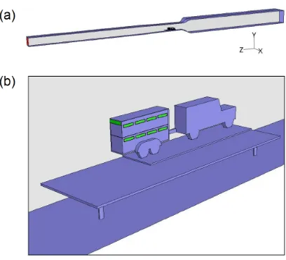
A series of wind tunnel tests was performed using a 1/7th scale model of a combined towing vehicle and

simplified livestock trailer, the latter constructed from Perspex panels to facilitate flow visualisation, see Fig.

1. The trailer had two separate decks, each with a series of eight rectangular vent apertures positioned on

the side panels. In addition, a large rear vent spanning the entire width of the trailer was placed above the

tailboard, Fig. 2.

Figure 1: Side view of the model towing vehicle and Perspex trailer in-situ within the wind tunnel.

Figure 2: Schematic diagram of the trailer showing the locations of the side vents, the rear vent and

pressure tappings.

The trailer was equipped with twenty-four pressure tappings, distributed on the left-hand side panel, the

tailboard and the roof; the positions of the tappings are indicated by the dots in the schematic diagram

shown in Fig. 2. The tappings were coupled to a multi-channel Sensor Technics pressure transducer which

particular experimental set up, the largest source of error in the measured pressures occurred due to the

limited resolution of the transducers giving an uncertainty inCp,ΔCp, of approximately 0.008.

Air velocity measurements were taken using a pitot tube which sampled the flow entering the vent

apertures, while a qualitative understanding of the flow structure was obtained using four rows of wool tufts,

which were mounted inside the trailer using wire rods. A viewing hole above the working section allowed

their movement to be recorded on video for subsequent analysis. The scale model was mounted inside the

tunnel’s working section using a groundboard to lift it above the tunnel floor’s boundary layer. The working

section tapered from 1.54m x 1.22m on entry to 1.58m x 1.28m on exit, with the model leading to a 3.4%

blockage (based on the average cross-sectional area of the working section). During the tests the

free-stream velocity was 19.2m/s, resulting in a Reynolds number of 1.74x106based on the combined length of

the vehicles. This is equivalent to 1/5th of the Reynolds number typically associated with a real, full-scale,

towing vehicle trailer combination negotiating narrow country roads in the United Kingdom. The free-stream

turbulence intensity was measured at 2.65% and this value was used in the CFD comparisons discussed

below.

3. CFD ANALYSIS OF WIND TUNNEL FLOWS: VERIFICATION AND VALIDATION

The scale model wind tunnel experiment described above was simulated using the commercial CFD

package, Fluent 6.3.26, which has recently been shown to be viable for predicting the flow field around

HGVs [7]. The solution domain, created within Fluent’s meshing package Gambit (version 2.3.16) consisted

of the tunnel’s upstream contraction zone, tapered working section and downstream duct, resulting in a

domain length of 9.2m. Preliminary analysis with this geometry highlighted the need to include uniform

upstream and downstream ducts such that the inlet and outlet boundaries were sufficiently far away from

the vehicle. These ducts were systematically lengthened to 20m until calculated surface pressures on the

trailer did not change significantly at the pressure tap locations, see Fig. 3(a); fully developed flow

conditions existed at the inlet and outlet.

The CFD mesh was decomposed into a series of zones with varying levels of refinement. Structured

quadrilateral cells were used throughout the domain, apart from the volume surrounding the towing vehicle

and trailer where unstructured tetrahedral grids were necessary to cope with geometrical complexity. Since

attention is restricted to steady-state solutions of symmetrical flow at zero yaw, a symmetry plane was

introduced to reduce the computational effort. Solution of the governing Navier-Stokes equations was

obtained using three different RANS-based turbulence models, namely the Spalart-Allmaras (SA) [9],

realizable k-ε (RKE) [10] and Menter’s SST k-ω (SSTKO) model [11]. These employed second order

discretization for the pressure equation and the QUICK [12] scheme for the momentum and turbulence

equations. The SIMPLE [13] pressure-velocity coupling algorithm was used together with double precision

Figure 3: (a) Final solution domain and (b) expanded view of the towing vehicle and trailer.

Solution convergence was established using the residual history and drag force monitors over a cycle of

10,000 iterations, although adequate convergence was generally observed after 3,000 iterations. Results

were obtained on three grids with differing levels of refinement applied to the external surfaces of the

towing vehicle and the trailer interior, resulting in cell counts of 2.33, 3.14 and 4.65 million respectively. The

grid structure surrounding the vehicles is shown in Fig. 4, with the coarse and fine grids near the tailboard

shown in Fig. 5. Standard wall functions were used together with no-slip boundary conditions on each wall

inside the flow domain. In all cases the y+ values were in the recommended range of between 30 and 300

[14].

Figure 5: Comparison between (a) coarse and (b) fine grid distribution near the trailer tailboard.

Two flow variables were chosen to compare the performance of each turbulence model on the three grids:

the combined drag coefficient of the towing vehicle and trailer,Cd, and the volumetric flow rate, Q, through

the rear vent aperture. Figure 6 shows that the drag coefficient predicted by each model is effectively

grid-independent, whereas the flow rate through the rear vent is a stronger function of grid density and the

turbulence model used. The latter is not surprising since the flow rate depends strongly on flow separation

around the trailer and the turbulence models treat the physics of boundary layer separation quite differently.

This finding is also consistent with previous studies which have shown that drag coefficients can be

predicted accurately using steady RANS models but that more complex regions of the flow require careful

grid resolution and/or time-dependent turbulence modelling [15,16]. It further highlights the importance of

experimental validation data from which the most appropriate turbulence model for a particular geometry

can be chosen.

0.5 0.6 0.7 0.8 0.9 1.0

2.0E+06 3.0E+06 4.0E+06 5.0E+06

Cell Count D ra g C o e ff ic ie n t Spalart Allmaras Realizable k-Epsilon SST k-Omega 0.000 0.005 0.010 0.015 0.020

2.0E+06 3.0E+06 4.0E+06 5.0E+06

Cell Count V o lu m e tr ic F lo w R a te (m ^ 3 /s ) Spalart Allmaras Realizable k-Epsilon SST k-Omega

Figure 6: Effect of grid refinement on drag coefficient and volumetric flow rate through the tailboard vent.

The grid-dependence of the solutions obtained can be quantified more precisely using Richardson

extrapolation [17,18] which predicts the accuracy of CFD predictions compared to ‘ideal’ values based on a

hypothetical zero grid spacing. Table 1 shows the grid-induced error in the flow rate through the rear vent

aperture using Richardson extrapolation. It can be seen that for the SA model the difference in predicted

flow rate between solutions found on the medium grid and fine grids is 1% while this figure increases to

1.7% when extrapolating to the ideal, zero grid spacing case. Note the much larger predicted errors for the

RKE and KO models.

Percentage Difference in Solutions

Turbulence Model Medium-to-fine Grid Spacing Medium-to-zero Grid Spacing

SA 1.0 1.7

RKE 19.1 34.4

KO 24.9 44.8

Table 1: Richardson extrapolation error estimates for flow rate as a function of grid level and turbulence

model.

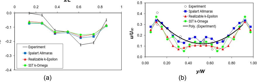
Figure 7 shows a comparison between wind tunnel experiments and CFD predictions obtained using the

medium grid structure. Cpvalues at the pressure tappings along the lower side of the trailer are shown in

Fig. 7(a). The predictions are all similar to each other and in reasonable agreement with those obtained

experimentally. Note that the measured value of Cpat the front is close to zero, suggesting well attached

flow, whereas the corresponding CFD predictions are negative, which indicates leading edge separation.

One possible reason for this is that the flows are very sensitive to leading edge sharpness: the CFD

analyses use completely sharp leading edges whereas the scale-model inevitably has some degree of

rounding. Comparisons of the velocity profile across the rear vent are shown in Fig. 7(b). Each turbulence

model predicts a profile lying to one side or the other of the experimental profile, however it is clear that the

SA one is generally closest to experiment with less scatter. Based on these findings and the above error

estimates, the SA turbulence model and the medium grid structure was used in all subsequent analyses.

-0.4 -0.3 -0.2 -0.1 0.0

0 0.2 0.4 0.6 0.8 1

x/L C p Experiment Spalart Allmaras Realizable k-Epsilon SST k-Omega 0.0 0.1 0.2 0.3 0.4 0.5

0.00 0.20 0.40 0.60 0.80 1.00

y/W u /U ¥ Experiment Spalart Allmaras Realizable k-Epsilon SST k-Omega Poly. (Experiment)

Figure 7: Comparison of experimental measurement and CFD predictions: (a) pressure along the lower side panels of the trailer; (b) velocity profile across the rear vent. The thick solid line in (b) is a third-order

polynomial fit to the experimental data.

TheCp plots shown in Figure 8 compare SA predictions against experiment, for the full range of pressure

tap locations shown in Fig. 2. Error bars for the experimental measurements were established from the

estimated errors in the transducer resolution. Figures 8(a) and (b) show a comparison of the side pressure

profiles; these agree reasonably well except at the rear of the upper deck, Fig 8(b). Here, the

experimentally obtained Cp value drops abruptly to -0.24 indicating flow separation, whereas the CFD

profile is almost flat with a smaller value of -0.10.

-0.4 -0.3 -0.2 -0.1 0.0

0 0.2 0.4 0.6 0.8 1

x/L C p Experiment Spalart Allmaras -0.4 -0.3 -0.2 -0.1 0.0

0 0.2 0.4 0.6 0.8 1

x/L C p Experiment Spalart Allmaras -0.4 -0.3 -0.2 -0.1 0.0

0 0.2 0.4 0.6 0.8 1

x/L C p Experiment Spalart Allmaras -0.4 -0.3 -0.2 -0.1 0.0

0 0.2 0.4 0.6 0.8 1

x/L C p Experiment Spalart Allmaras -0.4 -0.3 -0.2 -0.1 0.0

0.0 0.2 0.4 0.6 0.8 1.0

y/W C p Experiment Spalart Allmaras -0.4 -0.3 -0.2 -0.1 0.0

0.0 0.2 0.4 0.6 0.8 1.0

y/W

C

p

Experiment

Spalart Allmaras

Figure 8: Side pressure profiles along the (a) lower and (b) upper deck; roof pressure profiles: (c) outboard

and (d) centreline. Tailboard pressure profiles: (e) lower and (f) upper.

The profiles along the roof are in closest agreement, with partially attached flow evident, Figs. 8(c,d).

Tailboard pressures match well at the lower pressure tap locations, Fig 8(e); for the upper tailboard

pressures CFD significantly over-predicts separation at the outer edges, Fig 8(f). This discrepancy

highlights the difficulty in accurately predicting all the flow features occurring in the wake and is consistent

with the findings of previous studies using steady-state RANS turbulence models where the flow in the near

(c) (d)

(e) (f)

wake region can be very sensitive to the level of local grid refinement employed, and where better

agreement may require the use of unsteady RANS or LES methods [16]. However, despite the inherent

modelling limitations present within steady RANS approaches, the overall agreement presented above, is

good. Furthermore, the internal flow structure predicted from the CFD data is consistent with that observed

during flow visualisation experiments, as will be discussed.

4. RESULTS AND DISCUSSION

The aerodynamic and ventilation characteristics of the trailer are now investigated, including the effects of

introducing animals within the empty trailer and of making changes to the geometry of the towing vehicle.

Finally, Reynolds number effects are addressed via a brief analysis of the full-scale problem.

4.1 Scale-Model Analysis

A deeper analysis of the computed flow is presented, with particular emphasis placed on describing the

ventilation characteristics for the scale-model trailer which has the greatest relevance in relation to animal

welfare.

4.1.1 Drag

Recent substantial increases in fuel prices have brought the need for minimal aerodynamic drag into much

sharper focus [6]. For the case considered above, the combined drag coefficient for the scale-model towing

vehicle and trailer is 0.714, which equates to a total drag force of 7.66N. Of this total, approximately 40% is

attributable to the trailer. The various contributions to the total drag experienced by the scale-model trailer

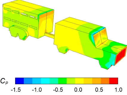
are given in Table 2. The headboard has by far the greatest contribution to trailer drag and closer analysis

of the internal flow field reveals that the dominant component of this is due to a region of low base pressure

behind the headboard (i.e. inside the trailer), not the stagnation pressure at the front of the headboard, as

might reasonably be expected. Note also that the percentage drag contribution from the underbody would

be significantly higher in practice due to the range of drag-inducing protuberances present on a real

vehicle. Surface contour plots of Cp shown in Fig. 9 highlight the stagnation regions with Cp ≈ 1.0

corresponding to the free-stream stagnation pressure.

Component Drag Contribution (%)

Headboard 65.7

Tailboard 20.4

Roof 1.4

Side Panel 2.5

Figure 9: Surface pressure distribution on the scale-model vehicles.

4.1.2 Internal Air Velocities and Flow Structure

When considering the flow patterns inside the trailer, the velocity field plays a significant role in dictating

where the air actually goes. Figure 10 shows velocity magnitude contour plots (normalized with respect to a

free-stream speed of 19.2m/s) in a horizontal plane at the mid-height of the vents in the lower and upper

decks. For the lower vent plane, air speeds are generally less than 10% of the free-stream, Fig 10(a). Here,

the highest air speeds are those arising from air ingestion through the front vents. This observation was

verified from the tuft movement seen in the experiments and the general flow structure from these

observations is depicted in Fig 11(a). There is a tendency for the free-stream to skip past the lower deck

with very little interaction between the internal and external flows.

Moving to the upper deck, the air speeds are not substantially higher than those on the lower deck, but

larger velocities are present in the rear half of the trailer, Fig 10(b). These elevated velocities are a result of

air from the free-stream entering the rear side vents and passing out through the top of the tailboard. In

fact, this passage of air serves to drive the internal flows in the direction of the free-stream with a more

clearly defined structure than that seen on the lower deck, Fig 11(b). Note that this flow regime is quite

different from that found for larger, single-unit animal transporters, where air is drawn into the rear of the

transporter in the opposite direction to the free-stream [1]. However, this can be explained by the different

layout of single-unit transporters. In such cases, the free-stream separates at the front of the box shape,

creating a very low external pressure around the front vent apertures thereby producing reversed internal

flow. Although not presented in this paper, further wind tunnel experiments were carried out for the

scale-model livestock trailer in isolation i.e. without the towing vehicle. The resulting flow structure was found to

be the same as for large transporters for the reasons outlined above, with pressure coefficients as low as

Figure 10: Computed normalized velocity magnitude contour plots when viewed from above: (a) lower vent

plane, (b) the upper vent plane.

Figure 11: Airflow patterns constructed from the experimental flow field when viewed from above: (a) lower

vent plane, (b) upper vent plane.

4.1.3 Passive Ventilation: Flow Rates

Though Figures 10 and 11 provide useful information on the internal airflow structure, it is difficult to assess

from this whether the ventilation is adequate on either deck. One way to do this quantitatively is to consider

the volumetric flow rates through all 9 vents before summing the ingoing (or outgoing) contributions. This

provides a simple, if relatively crude, calculation of the air exchange rate experienced on each deck, which

can then be converted into the number of air exchanges per hour, Nf. By characterizing the ventilation rate

non-dimensionally in this way, Nf is not exclusive to the scale-model. Results show that the number of air

exchanges is 1040/hour and 4668/hour for the lower and upper decks, respectively. Existing legislation

within the European Union specifies the minimum acceptable ventilation rate for livestock transporters to be

60m3/h/kN of livestock payload [20]. Based on a representative maximum payload of approximately 35kN

for small livestock trailers [21], this condition specifies a minimum air exchange rate of 1030m3/h per deck,

which is equivalent to 203 air exchanges per hour, per deck. Therefore, the results obtained from computed

flow fields of the scale-model livestock trailer show that the regulations are more than satisfied in this

instance.

The above result considers ventilation in terms of a ‘global’ air exchange rate for each deck. However, this

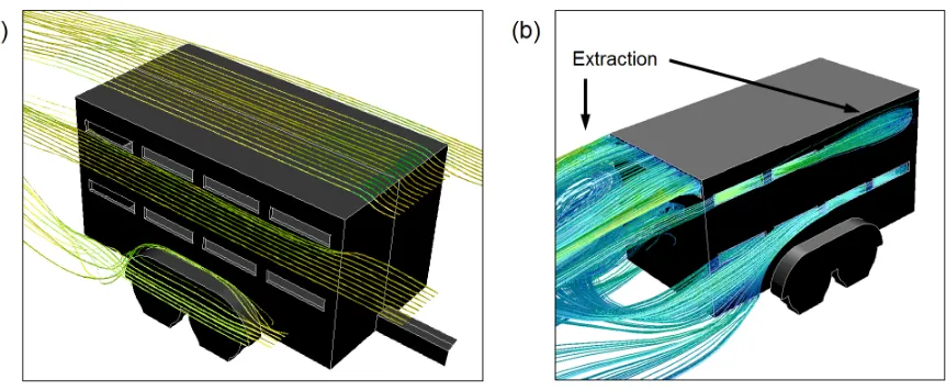
flow rate for each vent is represented by the equivalent number of air exchanges per hour. Overall, 80% of

the air entering the trailer flows through the top deck; there are two main reasons for this. Firstly, vent

number 5 at the front of the trailer extracts a significant volume of air due to the separated flows spilling

over the headboard, Fig. 13. Secondly, vent number 9, situated above the tailboard, provides a path for the

air simply to flow in through the side vents (6, 7 and 8) and directly out of the rear, see Figs. 13(b) and

11(b)

Figure 12 – Volumetric flow rates through the vent apertures.

Figure 13: (a) Pathlines in the external flow (b) from seeds released in each vent plane. The flow direction

is from right to left.

The efficiency of extraction through the rear vent is magnified by the negative base pressure occurring in

the wake. On the lower deck flow rates are considerably smaller due to the lack of an exit route on the

tailboard. Further, the lower half of the headboard is shielded from the free-stream by the towing vehicle,

which results in attached flows moving across the vent apertures. Although this flow regime is favourable in

terms of drag, the corresponding lack of suction around vent number 1 does limit ventilation and in fact

leads to a small air intake rather than the extraction seen on the upper deck. The small flow rate through

vent 2 and out of vent 3, as seen experimentally in Fig. 11(a). This is suggestive of a potential problem in

the local air exchange rate deeper inside the trailer in the region level with these forward vents.

4.1.4 Passive Ventilation: Residence Times

The main disadvantage of analysing flow rates through the vents is that they are situated on the extremities

of the vehicle and so the above results will inevitably be over-optimistic as they do not consider flow

behaviour deeper inside the trailer. No matter how much air enters the vents, there is no guarantee that all

regions will have adequate ventilation. One way to quantify air refreshment rate would be to fill the trailer

with a gas distinct from the ambient air and to measure its concentration over time as it is displaced by the

incoming air. This would be the computational equivalent of previous experimental work carried out on

horse-box trailer [5], but would require a time-dependent simulation. In the present study, estimates of local

air refreshment times throughout the trailer are obtained from steady-state analysis by releasing a total of

126 passive, mass-less tracer particles within each deck. Particle release points were evenly distributed in

a single horizontal plane on each deck, which intersected the side vent planes. A residence time was then

obtained for each particle, this being the time taken to travel through the trailer from the release point to the

point of exit. Ideally one should advect particles backwards in time to determine the time taken for fresh air

to reach the release point, but this was not possible within the version of the simulation software employed

here. However, since tracer particles were released throughout the planes considered, a conservation of

mass argument suggests that the maximum residence time calculated by forward advection to the point of

exit should be of a similar order to that calculated by backward advection to the point of entry.

Figure 14 is a contour plot of the residence time as a function of position through each tier of the trailer. On

the lower deck the maximum time taken for air to exit the trailer is approximately 19 seconds at a location

along the trailer centreline and a distance of one vent-width from the headboard. This indicates that the air

in this region is refreshed 190 times per hour, i.e. 5% below the previously mentioned limit of 203. In the

four corners of the lower deck the residence time is approximately 15 seconds but the overall average is

only 3.7 seconds, this being equivalent to 973 air exchanges per hour – close to the global value of Nf =

1040/hour established previously. Moving to the upper deck the maximum residence time is 8.1 seconds

situated behind the headboard, resulting in 444 air exchanges per hour. Taking an average value of 1.2

seconds gives an exchange rate of 3000 refreshments per hour. Overall, these figures reiterate the fact that

ventilation is significantly better on the upper deck. The most poorly refreshed area within the trailer occurs

Figure 14: Contour plots of residence time, trfor (a) the lower deck and (b) the upper deck. Particles were

released from the intersection points on each overlaid grid.

4.1.5 The Effect of the Presence of Animals

Under typical operating conditions, livestock trailers contain animals such as pigs or sheep. Clearly, the

effect that they have on the internal ventilation characteristics must be quantified and so a further

scale-model simulation was run. The presence of animals was accounted for as a blockage in the form of a wavy

surface assembled from a series of four longitudinal cylinders, see Fig 15.

Figure 15: Rendered CAD model of the livestock trailer containing simulated animals in the form of a (wavy

profiled) blockage on the upper and lower decks.

Results show that a greater volume of air flows through the trailer compared to one which is empty. The

number of air exchanges is increased by 1.4% and 22.5% for the lower and upper decks, respectively. This

observation is to be expected because the animals effectively take away the air volume in the lower half of

each deck but without blocking the vent apertures. Hence the corresponding reduction in volume promotes

faster airflow, leading to the increased air exchange rates seen. In a previous experimental study the

opposite effect was observed, however in this instance horses were transported and their height meant that

the vents were blocked [5]. The computed drag coefficient for the towing vehicle trailer combination

increased by 3.6% with animals present. This occurs by virtue of the increased viscous drag acting on the

4.1.6 Towing Vehicle Height

Another important aspect to consider is the effect of the shape of the towing vehicle on the internal

environment within the trailer. The motivation for doing this is that livestock trailers can be towed by

vehicles ranging from pick-up trucks to large SUV’s, where the main difference is the towing vehicle height.

A total of 6 different towing vehicle heights were explored with normalized height differences (h/H) ranging

from 0 to 0.5, Fig. 16.

Figure 16: Schematic illustration showing the different heights of the 6 towing vehicle-trailer combinations investigated.

Figure 17(a) shows how the drag coefficient contributions vary with the changes in towing vehicle height.

Minimum total drag occurs when the normalized height difference reaches 0.1, which incidentally was the

geometry used in the wind tunnel experiments. The drag force acting on the towing vehicle is generally

constant with the only noticeable increase occurring when there is no height difference, due to the

increased stagnation area. For small height differences the drag acting on the trailer headboard is small but

this increases by a factor of two as the trailer becomes more and more exposed to the free-stream.

0.0 0.3 0.6 0.9 1.2

0.0 0.1 0.2 0.3 0.4 0.5

h/H

C

d

Total Towing Vehicle Trailer - Headboard Trailer - Other

0 2000 4000 6000 8000 10000

0.0 0.1 0.2 0.3 0.4 0.5

h/H

Nf

L ower Deck Upper Deck

L ower Limit - F rom E U L egislation

Figure 17: Plots showing how (a) Cdand (b) Nfvary with the normalized height difference, h/H, between

the towing vehicle and trailer.

The number of air exchanges per deck was also plotted as a function of the height difference between the

two vehicles, Fig. 17(b). Interestingly, the volume of air passing through the upper deck increases for all

are of the same height (h/H = 0.0), the trailer headboard is completely shielded from the free-stream by the

towing vehicle which results in attached flows along the entire length of the trailer. Consequently more air

enters the side vents and the extraction originally seen through vent number 5 becomes an inflow for this

particular case. In contrast, when h/H is in the range 0.2-0.5, the headboard is far more exposed to the

free-stream, resulting in separated flows surrounding vent number 5. This leads to a much greater rate of

air extraction from the trailer which again increasesNfcompared with the original case. A similar pattern is

observed on the lower deck with increased flow rates occurring due to more air ingestion through the rear

two vents (3 and 4), and air extraction developing through vent number 1 ash/Hincreases. This shows that

a good ventilation rate can be achieved within the trailer for various towing vehicle heights.

4.2 Full-Scale Analysis

All of the above flow analysis is based upon scale-model vehicles confined within a wind tunnel, the

Reynolds Number, Re, of which is smaller than the equivalent full scale value. Thus a series of full-scale

simulations are presented which quantify the differences resulting from increasingRe.

4.2.1 Scaled-up Wind Tunnel Results

The free-stream velocity in the wind tunnel was 19.2m/s (~45Mph) which corresponds to typical full-scale

values, therefore this was kept constant. In order to simulate full-scale flows, all that remained was to

simply scale up the 1/7th scale model by a factor of 7. Firstly, this was done for the idealised wind-tunnel

flow considered above, allowing the differences between it and the scale-model to be compared. The first

two rows of data in Table. 3 show these differences.

Simulation Layout Scale U∞(m/s) Re Cd NL NU

Scale-model vehicle in wind tunnel 1/7 19.2 1.7 x 106 0.714 1040 4668

Full-scale vehicle in wind tunnel 1 19.2 1.2 x 107 0.681 147 679

Full-scale vehicle in free-air 1 19.2 1.2 x 107 0.701 135 786

Table 3: Comparison of drag and ventilation characteristics obtained for the scale model and full-scale

towing vehicle-trailer combination.

The total drag force and the number of air exchanges in the lower deck, NL, and the upper deck, NU, all

decrease as the scale increases. The difference in drag reduction is relatively small at 4.6% but the air

exchange rates are significantly smaller. In fact NL is reduced by a factor of 7.07 and NU by 6.87 which

entering the trailer is proportional to the vent area which has increased by 72, yet the volume inside the

trailer has increased by 73. It follows that the flow rates through the vents are a factor of 49 greater, but the

volume is in fact 343 times greater. Thus for the same flow speed, the full-scale trailer experiences air

exchange rates 1/7th those of the scale-model. Consequently, the scale-model results for ventilation are

over-optimistic by a factor of 7, whilst the drag is of a very similar magnitude.

4.2.2 Results With No Side-Wall Restrictions

Although the above findings are useful in determining how scale-model ventilation data translates to

full-scale situations, the presence confining walls in close proximity to the vehicles imposes unrealistic

boundary conditions on the airflow. Therefore CFD simulations for a full-scale vehicle were carried out with

a much taller and wider solution domain, to simulate motion in free-air i.e. tunnel walls removed. Wall-type

boundary conditions were imposed at these external boundaries but with full-slip characteristics to prevent

unrealistic boundary layer formation. These geometry changes resulted in a towing vehicle-trailer blockage

to the free-stream of just 0.4% compared with 3.4% experienced earlier. The results obtained are given as

the last row in Table. 3.

Drag is in the same range as for the previous two cases, suggesting that CFD simulations of small-scale

wind tunnel flows correlate very well with full-scale livestock trailers operating in free-air. Of course, the

same is not true for ventilation because of the aforementioned scaling effects, which lead to unrealistically

high ventilation rates in the trailer. More important is the correlation obtained between such data for a

full-scale vehicle in free-air and one in a full-full-scale wind tunnel. Results show that for the free-air case, a

reduction in NL of 8.1% is seen with an increase in NU of 15.8%. The increase on the upper deck is

attributable to the reduced blockage imposed by the vehicles on the surrounding column of air. This low

blockage allows air from the free-stream to spill more naturally around the trailer and thus enter the vents at

less-oblique angles. One effect of wind tunnel blockage is that air is squeezed between the trailer and

tunnel sidewalls, artificially aligning the flow in the longitudinal axis and thereby forcing it to flow past the

vent apertures. The reduction in air exchange rate on the lower deck is moderate but the lack of an exit

route on the tailboard does restrict the volume of air passing through this level of the trailer. It is not

unreasonable to assume that an increase in ventilation rate would likely be seen if a similar tailboard vent

to that on the upper deck was in place. This will be considered in a later study.

4.2.3 Sensitivity of Passive Ventilation to Vehicle Speed

Clearly, under realistic operating conditions, livestock trailers are towed at a variety of speeds. Hence a

range of air velocities. Figure 18 shows how the air exchange rate, Nf, on each deck varies for free-stream

velocities ranging from 4.5 – 22.3m/s (10 – 50mph).

0 200 400 600 800 1000

0.0 5.0 10.0 15.0 20.0 25.0

U_∞(m/s) Nf

L ower Deck Upper Deck

L ower L imit - F rom Legislation

Figure 18: Plot showing air exchange rates as a function of vehicle speed; full-scale computations.

The variation in Nf across this range of speeds follows a linear relationship on both decks with

approximately five times more air passing through the top deck than the bottom one. In terms of the

regulatory limit, ventilation can be considered acceptable on the upper deck but this is not the case on the

lower deck. Here, even at the highest vehicle speed of 22.3 m/s, the number of air exchanges is less than

the specified limit. For a typical operating speed of 13.4 m/s (30 mph) the deficit is 55%. Note also thatNf

does not account for localised regions which are poorly ventilated, and so the number of air exchanges in

5. CONCLUSIONS

Revealing the aerodynamic flow in and around a small livestock trailer is challenging both experimentally

and computationally due to the strong coupling between the internal and external flow fields. However, the

use of a coupled external/internal CFD analysis of the livestock trailer facilitates a detailed investigation of

the associated aerodynamic and passive ventilation characteristics. For the scale model under investigation

a good match is observed between the experimental and computational results, both in terms of external

pressure readings and qualitative aspects of the internal flow structure. Discrepancies are evident in the

near wake region behind the trailer, which is consistent with modelling issues identified by previous studies

[16]. Consequently future work will be required to generate additional experimental data and consider a

wider range of turbulence modelling and grid refinement strategies than it has been possible to address

here.

The CFD results for the scale-model highlight that air velocity fields, although useful in identifying regions of

slow-moving air, are not necessarily indicative of poor ventilation. Global air exchange rates can be

calculated from the sum of flows entering (or exiting) the trailer and are much more representative of the

ventilation characteristics. Exploitation of CFD to establish local air refreshment times gives the most

accurate representation of the true ventilation characteristics because it considers airflow behaviour

throughout the air volume. This technique is, however, sensitive to local aspects of the flow such as

recirculation regions, which in turn are sensitive to the turbulence model employed. Nevertheless,

residence times provide detail on the quality of ventilation deep inside the trailer which global air exchange

rates cannot.

A substantial increase in flow rate is evident on the upper deck with the inclusion of simplified animal

shapes; although variations in animal height around the vent apertures (i.e. from head shapes) were not

included, it is reasonable to assume that the inclusion of this feature would induce a further degree of

restricted airflow into the trailer immediately behind the vent apertures. This aspect may perhaps be worth

considering in future investigations. Analysis of different towing vehicle heights show that ventilation

characteristics are equally as pronounced whether the flow around the upstream vents is attached or

separated.

In addition to the scale-model analysis carried out, computations of the full-scale problem were performed,

leading to the following observations. Broadly speaking, the flow field is qualitatively unchanged and the

drag coefficient is insensitive to changes in scale, while the scale-model computations over-predict

ventilation by a factor of 7. Simulations of the full-scale problem show that in free-air, ventilation improves

on the upper deck, with some decrease on the lower deck. Further, ventilation varies linearly with vehicle

speed; while indications from the global number of air exchanges per hour suggest that the air is not

refreshed enough on the lower deck of the particular livestock trailer under investigation.

passive ventilation characteristics. Further studies are needed which take into account wind direction,

temperature and humidity in order to explore a wider range of possible conditions affecting welfare. The

priority in the short term is to assess the potential risks to welfare in extreme cases, such as when trailers

containing animals are stationary for long periods of time in hot conditions and passive ventilation is a

minimum. Work in these areas is currently ongoing.

Acknowledgements

The authors wish to acknowledge the financial support of the Department for Environment, Food and Rural

Affairs under Grant Reference Number AW0933, and Dr Janet Talling and Katja Van Driel of the Central

Science Laboratory for several stimulating and informative discussions on animal welfare issues. We are

also grateful to the livestock trailer manufacturer Ifor Williams for their assistance and advice throughout

this research project. Special thanks to Dr Summers for his time and commitment in ensuring the smooth

running of computer hardware for the CFD computations.

Nomenclature

Cp Pressure coefficient.

Cd Drag coefficient acting in the flow direction.

Q Volumetric airflow rate through the rear vent acting in the flow direction.

y+ Wall y-plus value for near-wall treatment.

r Grid refinement ratio.

x Distance along the length of trailer.

y Distance across width of trailer.

L Length of trailer.

W Width of trailer.

h Height difference between towing vehicle and trailer.

H Height of trailer.

Re Reynolds Number.

u Local Velocity.

U∞ Free-stream Velocity.

tr Particle residence time.

Nf Number of air exchanges per hour based on volumetric flow rates.

NL Number of air exchanges per hour for the lower trailer deck.

References

[1] Hoxey R P; Kettlewell P J; Meehan A M; Baker C J; Yang X. An investigation of the aerodynamic

and ventilation characteristics of poultry transport vehicles. Part I: Full scale measurements. Journal

of Agricultural Engineering Research, 65, 77-83, 1996.

[2] Kettlewell P J; Hoxey R P; Hampson C J; Green N R; Veale B M; Mitchell M A. Design and

operation of a prototype mechanical ventilation system for livestock transport vehicles. Journal of

Agricultural Engineering Research, 79, 429-439, 2002.

[3] Fisher A. D, Stewart M, Tacon J, Matthews L. R, The effects of stock crate design and stocking

density on environmental conditions for lambs on road transport vehicles, New Zealand Veterinary

Journal 50(4) 148-153, 2002.

[4] Friend T. H, Dehydration, stress, and water consumption of horses during long-distance commercial

transport, Journal of animal science, 78, pp 2568-2580, 2000.

[5] Pursewell J. L, Gates R. S, Lawrence L. M, Jacob J. D, Stombaugh T. S, Coleman R. J, Air

exchange rate in a horse trailer during transport, Proceedings of the 7th international symposium

livestock environment VII, Beijing, 2005, p13-20, ISBN 1892769484

[6] W.D. Pointer, T. Sofu, D. Weber, Development of guidelines for the use of commercial CFD in

tractor-trailer aerodynamic design, SAE paper 2005-01-3513, 2005.

[7] D. Gunes, Drag coefficient prediction analysis for heavy duty trucks, Progress in Computational

Fluid Dynamics, vol. 7, no. 8, 2007.

[8] W.D. Pointer, Evaluation of CFD code capabilities for prediction of heavy vehicle drag coefficients,

AIAA-2004-2254, 2004.

[9] Spalart P R, Allmaras S R. A one-equation turbulence model for aerodynamic flows. La Recherche

Aérospatiale, 1, 5-21, 1994.

[10] Shih T. H, A new k-epsilon eddy viscosity model for high Reynolds number flows, Computers in

Fluids, 24, pp 227-238, 1995.

[11] Menter F. R, Two-equation eddy-viscosity turbulence models for engineering applications, AIAA, 32,

pp1598-1605, 1994.

[13] Patankar S. V, Spalding D. B, A calculation procedure for heat, mass and momentum transfer in

three-dimensional parabolic flows. International Journal of Heat and Mass Transfer, 15, p 1787,

1972.

[14] Tu J, Computational Fluid Dynamics a practical approach, First Edition, Elsevier Inc, p262, 2008,

ISBN 9780750685634.

[15] R.C. McCallen, K. Salari, J.M. Ortega, L.J. DeChant, B. Hassan, C.J. Roy, W.D. Pointer, F.

Browand, M. Hammache, T-Y Hsu, A. Leonard, M. Rubel, P. Chatalain, S. Walker, R. Englar, J.

Ross, D. Satran, J.J. Heineck, S. Walker, D. Yaste, B. Storms, DOE’s effort to reduce truck

aeordynamics drag – joint experiments and computations lead to smart design, AIAA-2004-2249,

2004.

[16] C.J. Roy, J. Payne, M. McWheter-Payne, RANS simulations of a simplified tractor/trailer geometry,

J. Fluids Engineering, vol. 128, 1083-1089, 2006.

[17] Richardson L F. The deferred approach to the limit. Transactions of the Royal Society London, Ser

A, 226, 229-361, 1927.

[18] Roache P. J, Quantification of uncertainty in computational fluid dynamics, Annual review of fluid

mechanics, p126-160, 1997.

[19] Gilkeson C. A, Wilson M. C. T, Thompson H. M, Gaskell P. H, Barnard R. H, Hackett K. C, Stewart

D. H, Ventilation of small livestock trailers, 6th MIRA International Vehicle Aerodynamics

Conference, 2006, p138-147, ISBN 0952415631

[20] http://www.iwt.co.uk/brochures/livestock.pdf