This is a repository copy of Iterative learning control for constrained linear systems.
White Rose Research Online URL for this paper:
http://eprints.whiterose.ac.uk/74692/
Monograph:
Chu, B. and Owens, D.H. (2009) Iterative learning control for constrained linear systems.
Research Report. ACSE Research Report no. 990 . Automatic Control and Systems
Engineering, University of Sheffield
Reuse
Unless indicated otherwise, fulltext items are protected by copyright with all rights reserved. The copyright exception in section 29 of the Copyright, Designs and Patents Act 1988 allows the making of a single copy solely for the purpose of non-commercial research or private study within the limits of fair dealing. The publisher or other rights-holder may allow further reproduction and re-use of this version - refer to the White Rose Research Online record for this item. Where records identify the publisher as the copyright holder, users can verify any specific terms of use on the publisher’s website.
Takedown
If you consider content in White Rose Research Online to be in breach of UK law, please notify us by
Iterative Learning Control for Constrained
Linear Systems
Bing Chu, David H Owens
Department of Automatic Control and Systems Engineering,
University of Sheffield,
Mappin Street, Sheffield, S1 3JD, UK
Research Report No. 990
Department of Automatic Control and Systems Engineering
The University of Sheffield
Mappin Street, Sheffield,
S1 3JD, UK
Iterative Learning Control for Constrained Linear Systems
Bing Chu, David H Owens
aa
Department of Automatic Control and Systems Engineering The University of Sheffield, Mappin Street, Sheffield S1 3JD, UK
[email protected], [email protected]
Abstract
This paper considers iterative learning control for linear systems with convex control input constraints. First, the constrained ILC problem is formulated in a novel successive projection framework. Then, based on this projection method, two algorithms are proposed to solve this constrained ILC problem. The results show that, when perfect tracking is possible, both algorithms can achieve perfect tracking. The two algorithms differ however in that one algorithm needs much less computation than the other. When perfect tracking is not possible, both algorithms can exhibit a form of practical convergence to a ”best approximation”. The effect of weighting matrices on the performance of the algorithms is also discussed and finally, numerical simulations are given to demonstrate the effectiveness of the proposed methods.
Key words: iterative learning control; projection method; constraint handling; norm optimization
1 Introduction
Iterative learning control (ILC) is a control method for improving tracking performance of systems that execute the same task repeatedly by learning from the past ac-tions. Applications of ILC can be widely found in indus-trial robot manipulator, chemical batch process, some medical equipment and manufacturing, etc. Originating from robotics, ILC now attracts more general research interest [1], [2].
In many practical applications, the systems are under some constraints due to physical limitations or perfor-mance requirements. Hence, the ILC design must take these constraints into account. However, most of the cur-rent ILC research is based on assumed unconstrained systems and few results have been reported regarding the constrained case in the literature. [3] proposes a novel nonlinear controller for process systems with input constraints and the learning scheme only needs a little knowledge of the process model. [4] considers ILC prob-lem with soft constraints and uses Lagrange multiplier methods to solve this problem. [5] uses quadratic opti-mal design to formulate the constrained ILC problem and suggests quadratic optimal design has the capabil-ity of dealing with constraints.
In this paper, ILC design problem with general convex input constraints is discussed. It is shown that the con-strained ILC problem can be formulated in a recently
developed successive projection framework of ILC [6], which provides an intuitive but rigorous method for sys-tem analysis and design. Based on this, a syssys-tematic ap-proach for constraints handling is provided and two al-gorithms are proposed to solve this problem. The con-vergence analysis shows that when perfect tracking is possible, both algorithms can achieve perfect tracking whereas the computation of one algorithm is much less than the other at the cost of slightly slower convergence rate. When perfect tracking is not possible, both al-gorithms converge to asymptotic values representing a ”best fit” solution. Again the computational complex al-gorithm has the best convergence properties. It is also found that the input and output weighting matrices have an interesting effect on the convergence properties of the algorithms.
2 Problem Formulation
For simplicity, the formulation is described for linear dis-crete time systems but more generally applies to linear systems in Hilbert spaces described by equations of the
form y =Gu+d whereu, y are the system input and
output respectively,Gis a bounded linear operator from
an input Hilbert space to an output Hilbert space and
d represents other effects including the effect of initial
state conditions. For more details see [7]. Note that the abstract formulation describes many situations of inter-est including continuous linear state space model, dis-crete time model and differential delay model of system dynamics.
Consider the following discrete time, linear time-invariant system
xk(t+ 1) =Axk(t) +Buk(t)
yk(t) =Cxk(t), (1)
wheretis the time index (i.e. sample number),kis the
iteration number anduk(t), xk(t), yk(t) are input, state
and output of the system on iterationk. The initial
con-dition xk(0) =x0, k = 1,2,· · ·is the same for all
itera-tions. The control objective is to track a given reference
signalr(t) defined on a finite durationt∈[0, N] (i.e.tis
the sample number for time series of lengthN+1)and to
do so by repeated execution of the task and data trans-fer from task to task. Mathematically, at the final time
t=N, the state is reset tox0and time is reset tot= 0,
a new iteration is started and, again, the system is re-quired to track the same reference.
Before presenting the main results, the operator form of the dynamics is demonstrated using the well-known, so-called lifted-system representation, which provides a
straightforward ”N×Nmatrix” approach in the analysis
of discrete-time ILC [8], [9].
Assume, for simplicity, the relative degree of the system
is unity (i.e. the generic conditionCB6= 0 is satisfied),
then system model (1) on the kth iteration can be
ex-pressed in an equivalent form
yk=Guk+d, (2)
whereGanddare theN×N andN×1 matrices
G=
CB 0 · · · 0 0
CAB CB . .. 0 0
CA2B CAB . .. ... ...
..
. . .. ... CB 0
CAN−1B · · · · CAB CB
d=hCAx0 CA2x0 CA3x0 · · · CANx0
iT
. (3)
TheN×1 vectors of input, output and reference time
seriesuk, yk, rare defined as
uk=
h
uk(0) uk(1) · · · uk(N−1)
iT
yk=
h
yk(1) yk(2) · · · yk(N)
iT
r=hr(1) r(2) · · · r(N)
iT
(4)
andkrepresents the iteration number. As the most
im-portant signal vector is the tracking error vector e =
r−y, then, without loss of generality, it can be assumed
thatd= 0 by incorporating it into the reference signal
(i.e. replacingrbyr−d). Hence (2) becomes
yk =Guk, (5)
whereGis nonsingular and hence invertible.
The above representation of the original system (1) is called the lifted-system representation. This approach changes the original ILC problem into a MIMO tracking problem [8], [9]. Note that the above lifted-system form can be easily extended to situation when the system rel-ative degree is larger than one. All the following discus-sions will be based on the lifted-system representation.
Tracking error improvements from iteration to iteration are achieved in ILC using the following general control updating law
uk+1=f(ek+1, . . . , ek−s, uk,· · ·, uk−r), (6)
whereekis the tracking error from thekthtrial/iteration
and is defined as ek = r−yk. Whens > 0 or r > 0,
(6) is called a high order updating law. This paper only
considers algorithms of the formuk+1=f(ek+1, ek, uk).
For higher order algorithms, please refer to [10], [11] and the references therein.
The ILC Algorithm Design Problem:The ILC al-gorithm design problem can now be stated as finding a control updating law (6) such that the system output
has the asymptotic property thatek →0 ask→ ∞.
There are many design methods to solve the ILC prob-lem. The one used here is based on a quadratic (norm) optimal formulation [12] where, at each iteration, a per-formance index is minimized to obtain the system input time series vector to be used for that iteration. The ba-sis of this paper is Norm-Optimal ILC (NOILC) which uses the following performance index
Jk+1(uk+1) =kek+1kQ2 +kuk+1−ukk2R, (7)
minimized subject to the constraint that ek+1 = r−
Q andR are positive definite weighting matrices. Also
kek2
Q denotes the quadratic form eTQe and similarly
withk · k2
R. Solving this optimization problem gives the
following optimal choice for the time series vectoruk+1
uk+1=uk+R−1GTQek+1 (8)
which, when k → ∞, asymptotically achieves perfect
tracking. This well-known NOILC algorithm has many appealing properties including implementation in terms of Riccati state feedback. More details on NOILC can be found in [7], [12], [13], [14], [15].
In practical applications, system constraints are widely encountered. There are different kinds of constraints, e.g., input constraint, input rate constraint and state or output constraint. Constraints can be divided into two classes: hard constraints and soft constraints. Hard con-straints are concon-straints on magnitude(s) at each point in time, for example, the output limits on actuators. Soft constraints are constraints that are applied to the whole function rather than its point-wise values e.g. constraints on total energy usage. The input constraints are often hard constraints. This paper only considers the input constraint. Suppose the input is constrained to be in a
set Ω,which is taken to be a closed convex set in some
Hilbert space H. In practice, the set Ω is often simple
one. For example, the following constraints are often en-countered:
• Ω ={u∈H :|u(t)| ≤M(t)}
• Ω ={u∈H :λ(t)≤ |u(t)| ≤µ(t)}
• Ω ={u∈H : 0≤u(t)}
If there are no constraints, the ILC design problem is rel-atively easy to solve and there are many design methods in the literature. However, when constraints are present, the problem becomes more complicated. The problem is to decide how to incorporate the constraints into the de-sign process while retaining known performance proper-ties. In the following sections, the successive projection method proposed by Owens and Jones in [16] is used to interpret iterative learning control, and a systematic ap-proach for constraints handing in ILC is then proposed in the form of two new algorithms. The algorithms are related to but distinct from recently published work [6] where successive projection was used to accelerate norm optimal ILC.
3 Interpretation of ILC Using Successive Pro-jection
In this section, the concept of successive projection is summarised and its use in the ILC problem is demon-strated (for more details, please refer to [6] which uses the concepts to successfully accelerate norm optimal ILC). It is shown that the convex constrained ILC problem can
be formulated in the successive projection framework, the consequence of which is that a systematic approach for constraints handling is produced with known con-vergence properties. The notation in [16] is adopted in order to be consistent with the original paper and make the proof of our results more understandable. The nota-tionr, k, tis also used elsewhere in the paper to denote other variables, parameters or signals. This should cause no confusion as their meaning can be inferred from the context.
3.1 Successive Projection Method: An Overview
The successive projection method in the form described by Owens and Jones [16] is a technique for finding a
point in the (assumed non-empty) intersectionK1∩K2
of two closed, convex setsK1andK2in some real Hilbert
spaceH.The basic idea is to first select an initial iterate
k0inH. Subsequent points are obtained successively by
projection of previous iterates onto one and then the other of the two convex sets. It is formally described in the following theorem.
Theorem 1 [16] LetK1 ⊂ H, K2 ⊂ H, be two closed
convex sets in a real Hilbert spaceH withK1∩K2
non-empty. Define
Kj=
"
K1, j odd
K2, j even
Then, given the initial guess k0 ∈ H, the sequence
{kj}j≥0satisfying
kkj−kj−1k= min
k∈Kj
kk−kj−1k, j≥1 (9)
withkj ∈Kj, j≥1, is uniquely defined for eachk0∈H
and satisfies
kkj+1−kjk ≤ kkj−kj−1k, j≥2. (10)
Furthermore, for anyx∈K1∩K2,
kx−kjk2≥ kx−kj+1k2+kkj+1−kjk2 (11)
so that the sequence {kx−kj+1k}j≥0 is monotonically
decreasing and{kj}j≥0continuously gets closer to every
point inK1∩K2. In addition
∞
X
j=1
kkj+1−kjk2≤ kx−k1k2 (12)
so that, for each ǫ > 0, there exists an integer N such that forj≥N
inf
k∈Kj+1
k0
k1
k2
k3
K1∩K2
K1
K2
(a) Illustration of the Successive Projection Algo-rithm
k0 k1
k2 k3
e= 0
e=r−Gu
(0, u∗)
[image:6.595.61.266.220.341.2](b) Geometric Illustration of NOILC
Fig. 1. Successive Projection Interpretation of NOILC
That is, the iterateskj ∈Kj become arbitrarily close to
Kj+1.
Moreover, when K1∩K2 is empty, the algorithm
con-verges in the sense thatkkj+1−kjk →d(K1, K2)
defin-ing the minimum distanced(K1, K2)between the two sets
K1andK2.
The process is illustrated in Figure 1(a) which indicates convergence schematically to a point in the intersection
K1∩K2. In [16], this convergence is proved and a number
of related and improved iterative schemes are presented. Here, the one related to our ILC results is used. For more details please see [16].
3.2 Interpretation of ILC with Input Constraints
Consider the ILC design problem initially without con-straints. If the original system is injective, then for every
achievable r(t), there exists a unique input u∗(t) such
that r(t) = [Gu∗](t). The task of the ILC control law is
to iteratively find a series of inputs such thatuk →u∗
as k tends to infinity. That is equivalent to iteratively
finding the unique point (0, u∗)∈H =
RN ×RN in the
intersection of the following two sets inH:
• S1={(e, u)∈H :e=r−Gu}
• S2={(e, u)∈H :e= 0}
The successive projection method then can be applied to generate an algorithm with the defined convergence
properties. In general it is required to verify that these
two sets are closed and convex in H. This is trivially
satisfied, for example, in finite dimensional time series
spaces such as H = RN ×RN. In this case,the inner
product will be taken to be
h(e, u),(z, v)i=eTQz+uTRv (14)
with Q > 0, R > 0 symmetric positive definite
and the associated induced norm will be ||(e, u)|| =
p
h(e, u),(e, u)i.
Then, using successive projection method in Theorem 1, the well-known NOILC algorithm can be easily derived [6], which is illustrated geometrically in Figure 1(b). Its convergence properties can also be easily derived. For more details, please refer to [6].
Now consider the constrained ILC problem discussed in Section 2. The problem is to find the intersection of the
following closed, convex sets inH =RN×RN:
• S1={(e, u)∈H :e=r−Gu}
• S2={(e, u)∈H :e= 0}
under the constraint S3 ={(e, u)∈ H : u∈ Ω}. Note
that, it is normal thatS1∩S2∩S3is either a singleton
pair (e, u) = (0, u∗) solving the ILC problem or it is the
empty set∅. In this second case, perfect tracking is not
achievable due to the introducing of input constraint Ω.
There are three sets in the constrained problem. It seems the results in Owens and Jones [16] can not be directly
used. However, set S3 can be associated with either
S1 (yielding two sets S1 ∩ S3 and S2) or S2
(yield-ing two sets S2∩S3 and S1) and also notice that the
intersection of two closed convex sets is still a closed convex set. Then, the original 3-set problem becomes a 2-set problem, which is to find the intersection of
K1=S1(resp.S1∩S3) andK2=S2∩S3(resp.S2).
The successive projection method in Section 3.1 hence generates two new iterative algorithms for the con-strained ILC problem, which are demonstrated in the following two sections. In what follows, we do not spec-ify the exact form of the constraints other than that they are closed and convex.
4 Constrained ILC: Algorithm 1
This algorithm identifies that input constraints with the dynamics, a situation that explains why the algorithm is more computationally intensive than its alternative form (introduced later). The formal construction sets
K1=S1∩S3andK2=S2to be the closed convex sets
in Theorem 1, which can be described as follows.
r
0(
k
0)
r
1r
2(
k
1)
r
3e
= 0
e
=
r
−
Gu
(0
, u
∗)
(a) (S1∩S3)∩S26=∅and perfect tracking is possible
r
0(
k
0)
r
1r
2(
k
1)
r
3e
= 0
e
=
r
−
Gu
(0
, u
∗)
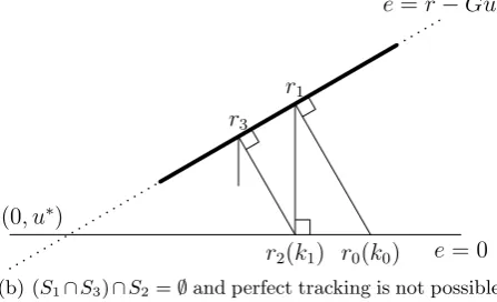
[image:7.595.51.275.227.363.2](b) (S1∩S3)∩S2=∅and perfect tracking is not possible
Fig. 2. Illustration of Algorithm 1
• K2={(e, u)∈H :e= 0}
The following algorithm can now be constructed and is illustrated schematically in Figure 2(a) and Figure 2(b), in which the cases when perfect tracking is possible (in-tersection occurs) or not (the in(in-tersection is empty)are shown, respectively.
4.1 Algorithm Description
Algorithm 1 Given any initial input u0 satisfying the
constraint with associated tracking error e0, the input
sequenceuk+1, k= 0,1,2,· · ·,defined by
uk+1= arg min
u∈Ω
n
kr−Guk2Q+ku−ukk2R
o
(15)
also satisfies the constraint and iteratively solves the con-strained ILC problem.
Proof. According to Theorem 1, let K1 = S1 ∩S3
and K2 = S2. Given r0 = (0, u0) ∈ K2, the sequence
{r1, r2,· · ·}given by
kri−ri−1k= inf
y∈Kj
ky−ri−1k, (16)
whereKj is defined as
Kj=
"
K1, j odd
K2, j even
,
iteratively finds the intersection ofK1andK2. The
sub-sequence{k1, k2,· · ·} ⊂K2defined by
kk=r2k, (17)
also iteratively finds the intersection ofK1andK2. That
is, it solves the ILC problem.
Note that,kk+1=r2(k+1)is solved by
kr2k+1−kkk= inf
y∈K1
ky−kkk (18)
and
kkk+1−r2k+1k= inf
y∈K2
ky−r2k+1k. (19)
Note that (18) is actually solving the following optimiza-tion problem
r2k+1: (ek+1, uk+1)
= arg min
(e,u)∈K1
©
ke−0k2
Q+ku−ukk2R
ª
, (20)
which is equivalent to solving
uk+1= arg min
u∈Ω
n
kr−Guk2Q+ku−ukk2R
o
(21)
and (19) simply gets kk+1 : (0, uk+1). That completes
the proof.
4.2 Convergence Analysis
This section discusses the convergence properties of Al-gorithm 1. As mentioned in Section 3.2, due to the
in-troducing of the input constraints Ω, there may be no
intersection ofS1, S2andS3,which means perfect
track-ing of the reference signal may be not possible. In this case, the convergence properties may have some differ-ence. Hence the convergence results are presented in two
parts: (S1∩S3)∩S26=∅and (S1∩S3)∩S2=∅.
4.2.1 (S1∩S3)∩S26=∅
Theorem 2 When perfect tracking is possible, Algo-rithm 1 can achieve monotonic convergence to zero tracking error, that is
kek+1k ≤ kekk, k= 0,1,· · ·. (22)
and
lim
k→∞ek = 0,k→∞lim uk =u ∗
. (23)
Proof. Monotonic convergence can be easily obtained
from the algorithm itself. Note that, atk+ 1 iteration,
the inputuk+1 is given by
uk+1= arg min
u∈Ω
n
kr−Guk2Q+ku−ukk2R
o
. (24)
Define
Jk+1(u) =kr−GukQ2 +ku−ukk2R. (25)
Then, it is easy to see
Jk+1(uk) =kekk2≥Jk+1(uk+1)
=kek+1k2+kuk+1−ukk2≥ kek+1k2 (26)
Hence we have
kek+1k ≤ kekk. (27)
Zero tracking error is got by noticing that Algorithm 1
iteratively finds the intersection of K1 = S1∩S3 and
K2 = S2, which is (0, u∗) when (S1∩S3)∩S2 6= ∅,
and hence, achieves perfect tracking. That completes the proof.
Algorithm 1 also has the desirable property that the
dis-tance between the kth input and the solutionu∗ is
de-creasing monotonically, as proved in the following theo-rem:
Theorem 3 When perfect tracking is possible, Algo-rithm 1 has the property that, for all k ≥0 and for all
u0andu∗
kuk+1−u∗k ≤ kuk−u∗k, (28)
i.e., the input iterates approach the solution monotoni-cally in norm.
Proof. According to Theorem 1 and the proof of
Algo-rithms 1, and given thatx∈K1∩K2= (0, u∗),then
kkk−xk2≥ kr2k+1−xk2≥ kkk+1−xk2. (29)
As x is (0, u∗), k
k is (0, uk) and kk+1 is (0, uk+1), it
immediately follows that
kuk+1−u∗k ≤ kuk−u∗k. (30)
as required.
4.2.2 (S1∩S3)∩S2=∅
In this case, perfect tracking is not possible. The al-gorithm does however compute an approximation of
the unconstrained inputu∗. For the convergence of the
tracking error, the following theorem holds.
Theorem 4 When perfect tracking is not possible, Al-gorithm 1 converges to pointu∗
swhich is uniquely defined
by the following optimization problem
u∗
s= arg min
u∈Ωkr−Guk 2
Q. (31)
Moreover, this convergence is monotonic in the tracking error, that is,
kek+1k ≤ kekk, k= 0,1,· · ·. (32)
Proof. According to Theorem 1, when (S1∩S3)∩S2=
∅, that is, perfect tracking can not be achieved,
Algo-rithms 1 will converge to pointu∗
s, where r1 = (e, u)∈
K1, r2= (0, u∗s)∈K2defining the minimum distance of
the two sets, which is the solution of the following opti-mization problem
(r1, r2) = arg min
r1∈K1,r2∈K2
kr1−r2k2. (33)
Remember the definition ofK1andK2,(33) is equivalent
to solve
(u, u∗s) = arg min
u∈Ω,u0
©
kr−Guk2Q+ku−u0k2R
ª
. (34)
Hence, Algorithm 1 converges to pointu∗
s, which is
de-fined by
u∗s= arg min
u∈Ω,u0
©
kr−Gu0k2Q+ku0−uk2R
ª
= arg min
u∈Ω
½ min
u0
kr−Gu0k2Q+ku0−uk2R
¾
. (35)
Notice that the inner minimization has the solution
u0=u. (36)
Hence, substitute (36) into (35) and the optimization problem can be transformed into
u∗s= arg min
u∈Ωkr−Guk 2
Note that G is invertible, then the performance index to be minimized is strictly convex, also notice that the constraint is convex, hence this quadratic programming problem has the unique solution.
The proof of monotonic convergence is similar to that of
(S1∩S3)∩S26=∅and is omitted here. That completes
the proof.
Remark 1 From the discussion above, it can be seen that Algorithm 1 has the appealing property of mono-tonic convergence of the tracking error. The main diffi-culty with Algorithm 1 is the solution of the constrained quadratic programming (QP) problem (15). In practice, the dimension of the time seriesukand plant operatorG
may be very large and the QP problem will be difficult or even become unmanageable. This is discussed in the next section and two methods are given as possible solutions.
4.3 Solution of the Subproblem
As mentioned above, the solving of the large QP problem is the main obstacle in applying Algorithm 1. In this section, two methods are given to solve the problem, that is, iterative solution and receding horizon method.
4.3.1 Using Iterative Algorithms
There are a number of iterative algorithms in the litera-ture to solve large scale QP problem, see [17], [18], [19], [20]. Here, the Goldstein-Levitin-Polyak (GLP) method is introduced [17], [18].
The GLP method minimizes a continuously
differen-tiable function f : H → R over a closed convex set
Ω⊂H using the iterative algorithm
xk+1=PΩ[xk−ak∇f(xk)], k= 0,1,· · · (38)
where PΩ(z) denote the projection of z ∈ H onto Ω,
∇f(xk) denotes the gradient off at xk andak ≥ 0 is
the step size and should satisfy
0< ǫ≤ak≤
2(1−ǫ)
L ,∀k (39)
whereLis a Lipschitz constant satisfying
|∇f(x)− ∇f(y)| ≤L|x−y|,∀x, y∈Ω. (40)
The convergence properties of this algorithm are also in-cluded in [17] and omitted here. One appealing property
is thatf(xk) will decrease monotonically, which is very
useful in ILC problem.
Algorithm 1 requires the solution of a QP problem, for which the gradient and the Lipschitz constant can be
easily got. Also notice that the constraint is rather simple and the projection can be carried on conveniently. Hence, the GLP method can be used to solve the QP problem arising in Algorithm 1. For the convergence property of this method, we have the following theorem.
Theorem 5 Using Goldstein-Levitin-Polyak method to solve the constrained QP problem, Algorithm 1 can main-tain monotonic convergence in the tracking error.
Proof. Define
Jk+1(u) =kr−Guk2Q+ku−ukk2R (41)
Then, at trialk+ 1, the algorithm minimizes the above
performance index subject to input constraints using Goldstein-Levitin-Polyak method and the initial point
isuk. Note that using Goldstein-Levitin-Polyak method,
Jk+1(u) will decrease monotonically. Suppose the
algo-rithm stops and gives thek+ 1thinputuk+1, we have
Jk+1(uk)≥Jk+1(uk+1), (42)
which is actually
kekk2≥ kek+1k2+kuk+1−ukk2. (43)
We immediately get
kekk ≥ kek+1k (44)
and that completes the proof.
Remark 2 In practice, due to the computational ex-penses, we can’t wait too many iterations to get the exact solution. Then, a prescribed maximum iteration or an expected accuracy can be given as criteria to terminate the GLP algorithm.
4.3.2 Receding Horizon Method
Another approach to solve the QP problem is using re-ceding horizon method, which is also noticed in [5]. The main idea is introduced here, and for more details please refer to [21].
At iteration k+ 1, the following problem needs to be
solved
uk+1= arg min
u∈Ω
n
kr−Guk2+ku−ukk
2o
(45)
The difficulty of this problem lies in the possible large
di-mension ofuandG.The receding horizon method,
(1) At timetand for the current statext, solve an
opti-mal control problem over a fixed future interval, say
[t;t+Nu−1], taking into account the constraints.
(2) Apply only the first step in the resulting optimal control sequence.
(3) Measure the state reached at timet+ 1.
(4) Repeat the fixed horizon optimization at timet+ 1
over the future interval [t+ 1;t+Nu], starting from
the (now) current statext+1.
Then, the original problem is reduced to a series of fol-lowing QP problems in Step 1:
uoptk+1,t= arg min
uk+1,t∈Ω
½t+Nu−1
P
i=t
kr(i)−yk+1(i)k2
+kuk+1,t(i)−uk(i)k2
o (46)
where
uk+1,t=
h
uk+1(t) uk+1(t+ 1) · · · uk+1(t+Nu−1)
iT
.
Note that this problem is of small size and can be solved easily.
The choosing ofNu is very important. IfNu=N,(46)
becomes the original problem (45). Large value of Nu
will give more accurate solution at the cost of large com-putational load while too small value may result in poor performance. There are a number of results in the liter-ature on how to choose the horizon, please refer to [21].
Note that, unlike Goldstein-Levitin-Polyak method, us-ing recedus-ing horizon control, Algorithm 1 may lose the monotonic convergence in the tracking error norm.
Remark 3 In this section, two methods are given to solve the large size constrained QP problem. There are also many other algorithms that can be used. It should be kept in mind that due to the practical restrictions, only an approximate solution of the QP problem can be got. Using this solution, the appealing convergence properties of Algorithms 1 may not be maintained, depending on the property of the methods used.
4.4 Effect of Weighting MatricesQandR
In this section, the effect of weighting matrices Qand
R on the convergence properties of Algorithm 1 is
dis-cussed.
According to (15), the weighting matricesQandR
pro-vide scaling on the tracking error and the change of
in-put. Intuitively, if Qis fixed, then a smallerR implies
larger acceptable change of input, and which in turn, re-sults in smaller tracking error. This leads to faster con-vergence rate.
0 5 10 15 20
−1 0 1
Time
ure
f
(
t
[image:10.595.318.526.80.262.2])
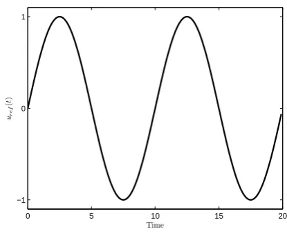
Fig. 3. The input signal
Consider SISO systems with scalar weightingQandR.
ChooseQ= 1 and consider the effect ofRon algorithm
performance. The following results can be easily derived. Whether perfect tracking is possible or not, it can be
expected (as with NOILC) that smallerRwill result in
faster convergence rate. The algorithm will converge to
the solution of (31), which is independent of R. This
implies that the weighting matrixRhas no effect on the
asymptotic accuracy but only affects the convergence rate. This is illustrated by the following example.
Example 1 Consider the following simple second order system
G(s) = s−4
s2+ 5s+ 6, (47)
which is sampled using a zero-order hold and a sampling time of 0.1s. The trial length is 20s, zero initial condi-tions are assumed and the reference signal is generated by the sine-wave inputu∗ shown in Figure 3. The
con-straint is taken to be|u(t)| ≤ 0.8, t= 0,1,· · ·, which is violated byu∗so that perfect tracking is not possible. The
initial input is chosen to beu0 = 0. The simulation is
designed to evaluate the effect of weighting matrices on the performance of Algorithm 1 over 100 iterations. Sim-ulations are run in six cases with weighting chosen to be
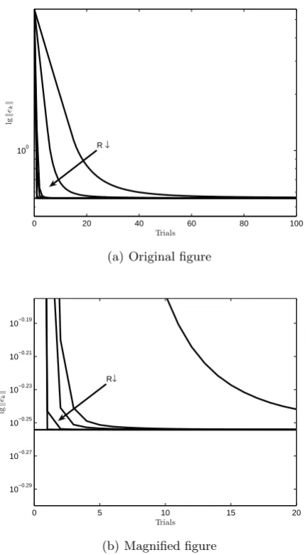
Q = 1and R = 3,1,0.1,0.05,0.01,0.001, respectively. The norms of the tracking error for each test are plotted and shown in Figure 4.
From the figure, it can be seen that the weighting matrix
Rhave no effect on the asymptotic accuracy. However,
smaller values of R result in faster convergence, which
verifies our expectations.
0 20 40 60 80 100 100
Trials
lg
k
ek
k
R ↓
(a) Original figure
0 5 10 15 20
10−0.29 10−0.27 10−0.25 10−0.23 10−0.21 10−0.19
Trials
lg
k
ek
k
R↓
(b) Magnified figure
Fig. 4. Effect of different weighting matrices on convergence performance
5 Constrained ILC: Algorithm 2
In this section, an alternative algorithm is given by
tak-ingK1=S1andK2=S2∩S3to be the closed, convex
sets in Theorem 1, which can be expressed as follows.
• K1={(e, u)∈H :e=r−Gu}
• K2={(e, u)∈H :e= 0, u∈Ω}
The following alternative algorithm to Algorithm 1 can be constructed and is illustrated schematically in Fig-ure 5(a) and FigFig-ure 5(b).
5.1 Algorithm Description
Algorithm 2 Given any initial input u0 satisfying the
constraint with associated tracking error e0, the input
r
0(
k
0)
r
1r
2(
k
1)
r
3e
= 0
e
=
r
−
Gu
(0
, u
∗)
(a)S1∩(S2∩S3)6=∅and perfect tracking is possible
r
0(
k
0)
r
1r
2(
k
1)
r
3e
= 0
e
=
r
−
Gu
(0
, u
∗)
[image:11.595.51.268.79.469.2](b)S1∩(S2∩S3) =∅and possible tracking is not possible
Fig. 5. Illustration of Algorithm 2
sequenceuk+1, k = 0,1,2,· · ·,defined by the solution of
the input unconstrained NOILC optimization problem
˜
uk= arg min
u
n
kr−Guk2Q+ku−ukk2R
o
(48)
followed by the simple input projection
uk+1= arg min
u∈Ωku−u˜kk ∈Ω (49)
also satisfies the constraint and iteratively solves the con-strained ILC problem.
Proof. According to Theorem 1, let K1 = S1 and
K2 = S2∩S3.Given r0 = (0, u0)∈ K2, the sequence
{r1, r2,· · ·}given by
kri−ri−1k= inf
y∈Kj
ky−ri−1k, (50)
whereKj is defined as
Kj=
"
K1, j odd
K2, j even
,
iteratively finds the intersection of K1 and K2. Then,
the sub-sequence{k1, k2,· · ·} ⊂K2 defined by
[image:11.595.314.537.208.353.2]also iteratively finds the intersection of K1 andK2 i.e.
it solves the ILC problem.
Note that,kk+1=r2(k+1)is solved by
kr2k+1−kkk= inf
y∈K1
ky−kkk (52)
and
kkk+1−r2k+1k= inf
y∈K2
ky−r2k+1k. (53)
Note that (52) is actually solving the following optimiza-tion problem
r2k+1: (˜ek,u˜k)
= arg min
(e,u)∈K1
©
ke−0k2
Q+ku−ukk2R
ª (54)
which is the solution of NOILC and (53) simply gives
kk+1: (0, uk+1),where
uk+1= arg min
u∈Ωku−u˜kk. (55)
That completes the proof.
Remark 4 Note that the second step of Algorithm 2 re-quires the solution of the problem (49). It seems this may need the application of some optimization methods. How-ever, in practice the input constraintΩis often a point-wise constraint and the solution of (49) can be computed easily. For example, whenΩ ={u∈H :|u(t)| ≤M(t)},
the solution is simply as follows,
uk+1(t) =
M(t) : ˜uk(t)> M(t)
˜
uk(t) :|u˜k(t)| ≤M(t)
−M(t) : ˜uk(t)<−M(t)
, (56)
fort= 0,· · ·, N−1.
5.2 Convergence Analysis
This section discusses the convergence properties of Al-gorithm 2. As for AlAl-gorithm 1, the results are presented
in two parts: (S1∩S3)∩S26=∅and (S1∩S3)∩S2=∅.
5.2.1 (S1∩S3)∩S26=∅
In this case, perfect tracking of the reference signal is
possible with a unique inputu∗. The theorem below
di-rectly follows from Theorem 1.
Theorem 6 When perfect tracking is possible, Algo-rithm 2 solves the ILC problem in the sense that
lim
k→∞ek = 0,k→∞lim uk =u
∗. (57)
Moreover, this convergence is monotonic with respect to the following performance index,
Jk =kEekkQ2 +kF ekk2R (58)
where
ek = r−Guk
E = I−G¡
GTQG+R¢−1
GTQ
F = ¡
GTQG+R¢−1
GTQ
. (59)
Proof. Equation (57) can be easily deduced from The-orem 1. Algorithm 2 iteratively finds the intersection
of K1 = S1 and K2 = S2∩S3, which is (0, u∗) when
S1∩(S2∩S3)6=∅, and hence, achieves perfect tracking.
Monotonic convergence with respect to the defined per-formance index can be obtained as follows. According to Theorem 1 and the proof of Algorithms 2, the distance
between{k0, r1, k1, r2,· · ·}is decreasing, that is
kkk−r2k+1k ≥ kr2k+1−kk+1k
≥ kkk+1−r2(k+1)+1k (60)
Note the left side is actually the minimum distance
be-tweenkkandK1, which is
kkk−r2k+1k= min
u
©
kr−Guk2Q+ku−ukk2R
ª
(61)
Note that this is the NOILC solution
ukr =uk+
¡
GTQG+R¢−1
GTQ(r−Gu). (62)
Substituting the solution, (61) can be further written as
kkk−r2k+1k= min
u
©
kEekk2+kF ekk2
ª
(63)
withE, F defined as (59). Note that this is performance
indexJk. Similarly, the right side of (60) isJk+1. Then
according to (60), we have
Jk+1≤Jk (64)
That is, performance indexJk is decreasing
monotoni-cally, which completes the proof.
0 5 10 15 20 −1
0 1
Time
ure
f
(
t
[image:13.595.55.266.73.460.2])
Fig. 6. The input signal
2 3 4 5 6 7 8 9 10 11
100.2 100.3 100.4 100.5 100.6 100.7
Trials
lg
k
ek
[image:13.595.60.265.81.249.2]k
Fig. 7. The tracking performance of Algorithm 2
It is well-known that NOILC achieves monotonic conver-gence in the tracking error. The following example shows that, Algorithm 2, however, may not have this property.
Example 2 Consider the following system
G(s) = 4.2130s−2.5164
s2−0.1312s+ 3.6624, (65)
which is sampled using a zero-order hold and a sampling time of 0.1s. The trial length is 20s, zero initial condi-tions are assumed and the reference signal is generated by the square-wave input shown in Figure 6. The con-straint is|u(t)| ≤1, t= 0,1,· · ·, which is satisfied by the inputu∗ so that perfect tracking is possible. The initial
input is chosen to be u0 = 0. The simulation evaluates
the performance of Algorithm 2 over 100 iterations. The weighting matrices are chosen to beQ=R=Ifor sim-plicity. The norm of the tracking error from2thto11th
iteration is plotted and shown in Figure 7.
From the figure, it is clear that Algorithm 2 may not pro-duce monotonic convergence in the tracking error norm.
Although Algorithm 2 may not maintain monotonic con-vergence in the tracking error, it has the property that
the distance between thekthinput and the optimal
so-lution is decreasing monotonically, which is shown in the following theorem.
Theorem 7 When perfect tracking is possible, Algo-rithm 2 has the property that, for allk ≥ 0 and for all
u0andu∗
kuk+1−u∗k ≤ kuk−u∗k, (66)
i.e., the input iterates approach the solution monotoni-cally in norm.
Proof. The proof is similar to that of Algorithm 1 and is omitted here.
5.2.2 (S1∩S3)∩S2=∅
In this case, perfect tracking is not possible and only an
approximation of the original inputu∗can be achieved.
The following theorem describes algorithm behaviour.
Theorem 8 When perfect tracking is not possible, Al-gorithm 2 converges to pointu∗
swhich is uniquely defined
by the following optimization problem,
u∗s= arg min
u∈Ω
©
kEek2Q+kF ek
2 R
ª
. (67)
Moreover, this convergence is monotonic with respect to the following performance index,
Jk =kEekkQ2 +kF ekk2R (68)
where
e =r−Gu E =I−G¡
GTQG+R¢−1
GTQ
F =¡
GTQG+R¢−1
GTQ
. (69)
Proof. According to Theorem 1, whenS1∩(S2∩S3) =
∅, that is, perfect tracking can not be achieved,
Algo-rithms 2 will converge to a pointu∗
s, wherer1= (e, u)∈
K1, r2 = (0, u∗s) ∈ K2 defining the minimum distance
between the two sets, which is the solution of the follow-ing optimization problem
(r1, r2) = arg min
r1∈K1,r2∈K2
Remember the definition ofK1andK2,(70) is equivalent
to solve
(u, u∗
s) = arg min
u∈Ω,u0
©
kr−Gu0k2Q+ku0−uk2R
ª
. (71)
Hence, Algorithm 2 converges to pointu∗
s, which is
de-fined by
u∗
s= arg min
u∈Ω,u0
©
kr−Gu0k2Q+ku0−uk2R
ª
= arg min
u∈Ω
½ min
u0
kr−Gu0k2Q+ku0−uk2R
¾
. (72)
Notice that the inner minimization is the solution of NOILC and is given by
u0=u+¡GTQG+R¢ −1
GTQ(r−Gu) (73)
Hence, substitute (73) into (72) and the optimization problem can be transformed into
u∗s= arg min
u∈Ω
©
kEek2
Q+kF ek2R
ª
(74)
where
e = r−Gu E = I−G¡
GTQG+R¢−1
GTQ
F = ¡
GTQG+R¢−1
GTQ
. (75)
Note thatEandF are invertible, then the performance
index to be minimized is strictly convex, also notice that the constraint is convex, hence this quadratic program-ming problem has unique solution.
The proof of monotonic convergence with respect toJk
is similar to that of Theorem 6 and omitted here, which completes the proof.
Remark 5 For the constrained ILC problem, the best result we can achieve in terms of tracking error is defined by the following QP problem
u∗= arg min
u∈Ωkr−Guk 2
. (76)
Compared to Theorem 8, it can be found that Algo-rithm 2 actually minimizes weighted norm of tracking error. In this case, only nearly optimal performance can be achieved.
5.3 Effect of Weighting MatricesQandR
In this section, the effect of weighting matrices Qand
R on the convergence properties of Algorithm 2 is
dis-cussed. As with Algorithm 1, the effect is illustrated in an intuitive way.
Consider SISO systems with scalar weighing QandR.
ChooseQ= 1 and consider the effect of variation ofR.
When perfect tracking is possible, perfect tracking can
be achieved and smaller R will result in faster
conver-gence. When perfect tracking is not possible, reducing
R will again result in faster convergence rate but the
asymptotic error changes (in contrast to Algorithm 1). This can be explained as follows. Algorithm 2 converges to the solution of the following problem
u∗
s= arg minu∈Ω
n
k(I−G¡
GTQG+R¢−1
GTQ)ek2 Q
+k¡
GTQG+R¢−1
GTQek2 R
o
WhenR → ∞, the first term of the last equation
be-comeskek2
Q and the second term becomes zero. Hence,
the optimization problem becomes
u∗
s= arg min
u∈Ωkek 2
Q (77)
This is the constrained optimal solution and is the best result that can be achieved with constrained control. However, in this case, since the weighting of input change
R is very large, the convergence rate is expected to be
very slow. One the other hand, whenR →0,it can be
seen the first term of the last equation becomes zero
and the second term becomes kG−1ek2
R, which can be
further written asku−u∗k2
R,whereu∗is the unique input
generating the reference signal. Hence, the optimization problem becomes
u∗
s= arg min
u∈Ωku−u ∗k2
R (78)
This is just the projection ofu∗onto the constraint set
Ω. Clearly the tracking error may be larger than that of the constrained optimal solution. However, in this case, the convergence rate is fast.
From the discussion above, it can be seen that when
per-fect tracking is not possible, the weighting matrixR
pro-vides a compromise between the convergence rate and the tracking performance, which is very different from that of Algorithm 1. This is illustrated in the following example.
Example 3 Consider the following system
G(s) = s+ 4
s2+ 5s+ 6, (79)
which is sampled using a zero-order hold and a sampling time of 0.1s. The trial length is 20s, zero initial condi-tions are assumed and the reference signal is generated by the sine-wave input shown in figure 3. The constraint set is defined by|u(t)| ≤0.8, t= 0,1,· · ·, which doesn’t con-tain the inputu∗. The initial input is chosen to beu
0 50 100 150 200 100
Trials
lg
k
ek
k
R ↓
(a) Original figure
0 20 40 60 80 100
10−0.29 10−0.26 10−0.23 10−0.2 10−0.17 10−0.14 10−0.11
Trials
lg
k
ek
k
R↑
(b) Magnified figure
Fig. 8. Effect of different weighting matrices on convergence performance
The simulation aims to investigate the effect of weight-ing matrices on the performance of Algorithm 1 over 100 iterations. Six simulations are shown with the weighting matrices Q = I and R = 3,1,0.1,0.05,0.01,0.001, re-spectively. The results are shown in Figure 8 and Fig-ure 9.
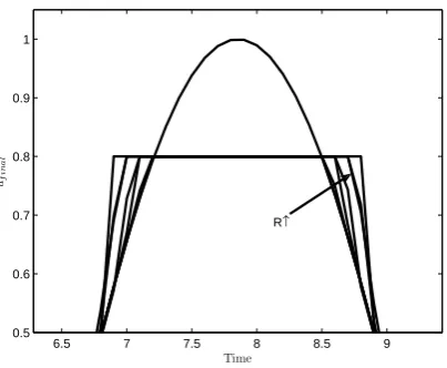
From the figure, it can be seen that smaller R results in faster convergence and the weighting matrix R does have an effect on the asymptotic performance/accuracy with larger values of R giving smaller asymptotic er-ror norms. The asymptotic tracking erer-ror norm of Al-gorithm 2 against different weighting matricesR is also plotted and shown in Figure 10. Note that the lower hori-zonal line is the tracking error norm with the input (77) and the upper one is (78).
When the system is MIMO or the weighting matrices are not scalar, the effect of weighting matrices would
6.5 7 7.5 8 8.5 9
0.5 0.6 0.7 0.8 0.9 1
Time
uf
in
a
l
[image:15.595.323.525.81.247.2]R↑
Fig. 9. Part of the resulting input
10−6 10−4 10−2 100 102 104 106 0.57
0.58 0.59 0.6 0.61 0.62 0.63
Input WeightingR
As
y
m
p
to
ti
c
V
a
lu
e
k
e
k
Fig. 10. Effect of different weighting matrices on asymptotic performance
not be so easy to analyze but a similar pattern could be expected.
6 Numerical Simulation
In this section, three examples are given to demonstrate the effectiveness of the proposed methods. First, con-sider the following example where perfect tracking is achievable.
Example 4 Consider the following non-minimum phase system
G(s) = s−4
s2+ 5s+ 6, (80)
[image:15.595.51.270.82.468.2] [image:15.595.328.526.282.455.2]0 5 10 15 20 −1
0 1
Time
ure
f
(
t
[image:16.595.318.526.76.248.2])
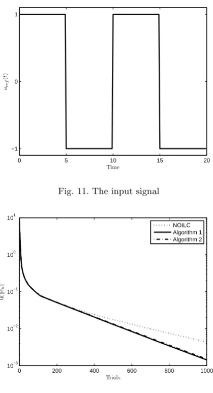
Fig. 11. The input signal
0 200 400 600 800 1000
10−3 10−2 10−1 100 101
Trials
lg
k
ek
k
[image:16.595.56.266.78.465.2]NOILC Algorithm 1 Algorithm 2
Fig. 12. Comparison of convergence
the square-wave input shown in figure 11. The constraint
is|u(t)| ≤ 1, t = 0,1,· · ·, which just contains the input
u∗. The initial input is chose to beu
0= 0. The
simula-tion compares the NOILC, Algorithm 1 and Algorithm 2 with over 1000 iterations. For simplicity, the weighting matrices are chosen to be Q =R = I.The results are shown in Figure 12 and Figure 13.
Note that in this example, perfect tracking is possible. According to Theorem 2 and Theorem 6, perfect track-ing can be achieved by both algorithms. However, it is expected that the constraint will be active during the iter-ations, which means the resulting input of NOILC may violate the constraint.
From Figure 12, it can be seen that Algorithm 1 and Al-gorithm 2 is approaching perfect tracking, which verifies the previous expectations. During the first iterations, as
u0 = 0,uk increases in point-wise magnitude gradually
and doesn’t violate the constraint in any of the three al-gorithms. In subsequent iterations, the input computed
0 5 10 15 20
−2 −1.5 −1 −0.5 0 0.5 1 1.5
2x 10 −3
Time
efin
a
l
(
t
)
NOILC Algorithm 1 Algorithm 2
Fig. 13. The tracking error at 1000th
iteration
using NOILC then begins to violate the constraint and differences begin to emerge. It is interesting to see that Algorithm 1 and Algorithm 2 outperform NOILC at this stage. It can also be seen that Algorithm 1 performs a little better than Algorithm 2.
The second example is to illustrate what will happen if perfect tracking is not possible.
Example 5 Consider the same non-minimum phase system
G(s) = s−4
s2+ 5s+ 6, (81)
which is sampled using a zero-order hold and a sampling time of 0.1s. The trial length is 20s, zero initial condi-tions are assumed and the reference signal is generated by the sine-wave input as shown in Figure 14. The con-straint is replaced by|u(t)| ≤0.8, t= 0,1,· · ·, so that per-fect tracking is not possible. The initial input is chosen to beu0 = 0. The simulation compares Algorithm 1,
Algo-rithm 2 and the constrained optimal (76) over 200 itera-tions. The weighting matrices are chosen to beQ=R=I
for simplicity. In Algorithms 1, the constrained QP prob-lem is solved by the Matlab optimization toolbox. The re-sults are shown in Figure 15, Figure 16 and Figure 17.
[image:16.595.61.265.81.249.2]0 5 10 15 20 −1
0 1
Time
ure
f
(
t
[image:17.595.314.527.80.248.2])
Fig. 14. The input signal
0 50 100 150 200
100
Trials
lg
k
ek
k
Algorithm 1 Algorithm 2 Constrained Optimal
(a) Original figure
0 50 100 150 200
10−0.19 10−0.17 10−0.15 10−0.13 10−0.11 10−0.09
Trials
lg
k
ek
k
Algorithm 1 Algorithm 2 Constrained Optimal
[image:17.595.52.268.102.687.2](b) Magnified figure
Fig. 15. Comparison of convergence
0 5 10 15 20
−0.2 −0.15 −0.1 −0.05 0 0.05 0.1 0.15
Time
efin
a
l
(
t
)
Algorithm 1 Algorithm 2 Constrained Optimal
Fig. 16. The tracking error at 200th
iteration
0 5 10 15 20
−1 −0.8 −0.6 −0.4 −0.2 0 0.2 0.4 0.6 0.8 1
Time
uf
in
a
l
(
t
)
Algorithm 1 Algorithm 2 Constrained Optimal Original Input
Fig. 17. The resulting input at 200th
iteration
on the original input, instead, it adds some compensa-tion. It should be kept in mind that although Algorithm 1 gives better performance, this is achieved at the expense of large computation load, which may be not acceptable in the real application, whereas Algorithm 2 achieves nearly optimal performance using quite simple computation.
The third example is to illustrate alternative solution methods of Algorithm 1 when perfect tracking is not possible.
Example 6 Again, consider the same non-minimum phase system
G(s) = s−4
s2+ 5s+ 6, (82)
[image:17.595.317.527.289.454.2]0 50 100 150 200 100
Trials
lg
k
ek
k
GLP method Receding Horizon method Quadratic Programming Constrained Optimal
(a) Original figure
0 50 100 150 200
10−0.19 10−0.17 10−0.15 10−0.13 10−0.11 10−0.09
Trials
lg
k
ek
k
GLP method Receding Horizon method Quadratic Programming Constrained Optimal
[image:18.595.313.526.80.249.2](b) Magnified figure
Fig. 18. Comparison of convergence
doesn’t contain the original input and implies that perfect tracking is not possible. The initial input is chosen to be
u0= 0. The simulation compares the iterative algorithm,
receding horizon method and exact solution of the con-strained QP problem of Algorithm 1 over 200 iterations. The exact solution is solved by Matlab optimization tool-box. The weighting matrices are chosen to beQ=R=I.
In the iterative algorithm, the algorithm is stopped after 10 iteration. In the receding horizon control method, the horizon is chosen to beNu = 10.The results are shown
in Figure 18, Figure 19 and Figure 20.
From Figure 18, it can be seen that, the iterative solution method converges to the constrained optimal solution as
k→ ∞,while the receding horizon method doesn’t. This is due to the solution accuracy of the receding horizon method. Further simulation shows that when improving the accuracy of the solution by increasing the horizon in the receding horizon method, the limiting point become closer to the constrained optimal solution. It can also be
0 5 10 15 20
−0.2 −0.15 −0.1 −0.05 0 0.05 0.1 0.15
Time
efin
a
l
(
t
)
[image:18.595.52.270.82.469.2]GLP method Receding Horizon method Quadratic Programming Constrained Optimal
Fig. 19. The tracking error at 200th
iteration
0 5 10 15 20
−1 −0.8 −0.6 −0.4 −0.2 0 0.2 0.4 0.6 0.8 1
Time
uf
in
a
l
(
t
)
GLP method Receding Horizon method Quadratic Programming Constrained Optimal Original Input
Fig. 20. The resulting input at 200th
iteration
noticed that the convergence rates of iterative solution method and receding horizon control method are lower than that of the exact solution of constrained QP prob-lem. The convergence rate can be further improved by in-creasing the iteration number in the iterative solution or by enlarging the horizon in the receding horizon method.
7 Conclusion
[image:18.595.318.526.290.456.2]computational effort. When perfect tracking is not pos-sible, both algorithms have been shown to provide use-ful approximate solutions to the constrained ILC prob-lem but that (1) the asymptotic error will be non-zero and (2) the computational complexity and convergence properties of the algorithms do differ. These observa-tions should be taken into account when choosing the al-gorithm, which requires a compromise between the per-formance/accuracy and the computational cost. The ef-fect of weighting matrices on the performance of the al-gorithms has also been discussed and numerical simula-tions have been given to demonstrate their effectiveness.
For completeness, two methods are proposed to solve the large scale QP problem arising in Algorithm 1. However, a more accurate and faster solver would be useful. This topic is worthy of further development. There is also more work that needs to be done to extend the results in this paper to nonlinear systems.
Finally, although the presentation has concentrated on sampled data systems (for reasons of both simplicity and practical relevance), the Hilbert space context of succes-sive projection indicates that the ideas and results apply more widely and, in particular, to the case of continu-ous time systems with no change in the abstract form of the algorithms or results. The realization of these results will however change.
References
[1] D.H. Owens and J. Hatonen. Iterative learning control - an optimization paradigm. Annual Reviews in Control, 29(1):57–70, 2005.
[2] D.A. Bristow, M. Tharayil, and A.G. Alleyne. A survey of iterative learning control: A learning-based method for high-performance tracking control. IEEE Control Systems Magazine, 26(3):96–114, 2006.
[3] C.T. Chen and S.T. Peng. Learning control of process systems with hard input constraints. Journal of Process Control, 9(2):151–160, 1999.
[4] S. Gunnarsson and M. Norrlof. On the design of ILC algorithms using optimization. Automatica, 37(12):2011– 2016, 2001.
[5] J.H. Lee, K.S. Lee, and W.C. Kim. Model-based iterative learning control with a quadratic criterion for time-varying linear systems. Automatica, 36(5):641–657, 2000.
[6] B. Chu and D. H. Owens. Accelerated norm-optimal iterative learning control algorithms using successive projection.
International Journal of Control, to appear, 2008.
[7] N. Amann, D.H. Owens, and E. Rogers. Iterative learning control using optimal feedback and feedforward actions.
International Journal of Control, 65(2):277–293, 1996.
[8] J. Hatonen. Issues of algebra and optimality in iterative learning control. PhD thesis, University of Oulu, Finland, 2004.
[9] J.J. Hatonen, D.H. Owens, and K.L. Moore. An algebraic approach to iterative learning control.International Journal of Control, 77(1):45–54, 2004.
[10] Z. Bien and K.M. Huh. Higher-order iterative learning control algorithm. IEE Proceedings, Part D: Control Theory and Applications, 136(3):105–112, 1989.
[11] J. Hatonen, D.H. Owens, and K. Feng. Basis functions and parameter optimisation in high-order iterative learning control. Automatica, 42(2):287–294, 2006.
[12] N. Amann, D.H. Owens, and E. Rogers. Predictive optimal iterative learning control. International Journal of Control, 69(2):203–226, 1998.
[13] N. Amann.Optimal algorithms for iterative learning control. PhD thesis, University of Exeter, UK, 1996.
[14] N. Amann and D.H. Owens. Non-minimum phase plants in norm-optimal iterative learning control. Report, University of Exeter, 1994.
[15] N. Amann, D.H. Owens, and E. Rogers. Iterative learning control for discrete-time systems with exponential rate of convergence. IEE Proceedings: Control Theory and Applications, 143(2):217–224, 1996.
[16] D. H. Owens and R. P. Jones. Iterative solution of constrained differential/algebraic systems. International Journal of Control, 27(6):957–974, 1978.
[17] A.A. Goldstein.Constructive real analysis. New York: Harper & Row, 1967.
[18] D.P. Bertsekas. On the Goldstein-Levitin-Polyak gradient projection method. IEEE Transactions on Automatic Control, 21(2):174–183, 1976.
[19] M. Bierlaire, P.L. Toint, and D. Tuyttens. On iterative algorithms for linear least-squares problems with bound constraints.Linear Algebra and Its Applications, 143(1):111– 143, 1991.
[20] B.S. He. A projection and contraction method for a class of linear complementarity-problems and its application in convex quadratic-programming. Applied Mathematics and Optimization, 25(3):247–262, 1992.