Optimal modelling and experimentation for the improved sustainability of microfluidic chemical technology design

This is a repository copy of Optimal modelling and experimentation for the improved sustainability of microfluidic chemical technology design.

White Rose Research Online URL for this paper: http://eprints.whiterose.ac.uk/8907/

Article:

Zimmerman, W.B. and Rees, J.M. (2009) Optimal modelling and experimentation for the improved sustainability of microfluidic chemical technology design. Chemical Engineering Research and Design, 87 (6A). pp. 798-808. ISSN 0263-8762

https://doi.org/10.1016/j.cherd.2008.11.010

eprints@whiterose.ac.uk https://eprints.whiterose.ac.uk/ Reuse

Unless indicated otherwise, fulltext items are protected by copyright with all rights reserved. The copyright exception in section 29 of the Copyright, Designs and Patents Act 1988 allows the making of a single copy solely for the purpose of non-commercial research or private study within the limits of fair dealing. The publisher or other rights-holder may allow further reproduction and re-use of this version - refer to the White Rose Research Online record for this item. Where records identify the publisher as the copyright holder, users can verify any specific terms of use on the publisher’s website.

Takedown

If you consider content in White Rose Research Online to be in breach of UK law, please notify us by

* Manuscript

Optimal modelling and experimentation for the improved

sustainability of microfluidic chemical technology design.

1 2

WB Zimmerman and JM Rees

1

Department of Chemical and Process Engineering ;

2

Department of Applied Mathematics , University of Sheffield, Sheffield S10 2TN

Abstract

Optimization of the dynamics and control of chemical processes holds the promise of improved sustainability for chemical technology by minimising resource wastage. Anecdotally, chemical plant may be substantially over designed, say by 35-50%, due to designers taking account of uncertainties by providing greater flexibility. Once the plant is commissioned, techniques of nonlinear dynamics analysis can be used by process systems engineers to recoup some of this overdesign by optimisation of the plant operation through tighter control. At the design stage, coupling the experimentation with data assimilation into the model, whilst using the partially informed, semi-empirical model to predict from parametric sensitivity studies which experiments to run should optimally improve the model. This approach has been demonstrated for optimal experimentation, but limited to a differential algebraic model of the process. Typically, such models for online monitoring have been limited to low dimensions.

Recently it has been demonstrated that inverse methods such as data assimilation can be applied to pde systems with algebraic constraints, a substantially more complicated parameter estimation using finite element multiphysics modelling. Parametric sensitivity can be used from such semi-empirical models to predict the optimum placement of sensors to be used to collect data that optimally informs the model for a microfluidic sensor system. This coupled optimum modelling and experiment procedure is ambitious in the scale of the modelling problem, as well as in the scale of the application – a microfluidic device. In general, microfluidic devices are sufficiently easy to fabricate, control, and monitor that they form an ideal platform for developing high dimensional spatio-temporal models for simultaneously coupling with experimentation.

As chemical microreactors already promise low raw materials wastage through tight control of reagent contacting, improved design techniques should be able to augment optimal control systems to achieve very low resource wastage. In this paper, we discuss how the paradigm for optimal modelling and experimentation should be developed and foreshadow the exploitation of this methodology for the development of chemical microreactors and microfluidic sensors for online monitoring of chemical processes. Improvement in both of these areas bodes to improve the sustainability of chemical processes through innovative technology.

§1 In

troduction

The purpose of this aper is to forecast current trends in microfluidics concerning sustainable microfluidic chemical design. The application areas of microfluidics which are currently successful are heavily dominated by “labs-on-a-chip” implementations of chemical and biochemical analyses, for which the likely future extrapolation is individual medicine based on “path-labs-on-a-chip”. Sustainability, however, is an issue for the other two major potential uses of microfluidics on microchips – microreactors and microfluidic sensors. To our knowledge, there are no mass produced chemical microreactors for large scale production of fine chemicals or pharmaceuticals by “scale out”: the duplication of microreactors fed reactants by a distributor system and collection of the products by a centralized harvesting system. Similarly, we know of no mass produced sensor systems that are microchip based for sampling fluid systems and reporting online variations of the sensed quantity. How is it that the undoubted success of microchip-based microfluidics for high throughput screening has not yet translated through to these other two promising areas?

To answer this, we should first learn the lessons of why high throughput screening, especially in biotech applications, has worked. On the surface, it would appear to be a harmony of scale between the manipulation advantage afforded by onchip microfluidics and the target objects:

This is an author produced version of Zimmerman, W.B. and Rees, J.M. (2009) Optimal modelling and experimentation for the improved sustainability of microfluidic chemical technology design. Chemical Engineering Research and Design, 87 (6A). pp. 798-808.

cells and microorganisms, subcellular organelles and biomacromolecules. Furthermore, there is an inherent handling advantage in the ability to manipulate small quantities of fluids when there are only small quantities (e.g. nanolitres) of the (bio)materials available. Futhermore, microfluidics offers organizing or processing principles not typically used in biotech/biochem analysis: fluid transport, flow and fluid structures. In short, the specific capabilities of microfluidic processing are advantages to labs-on-a-chip for high throughput biotech screening, as well as certain fine chemicals, which are not so easily implemented at higher scales. For a recent review of the micro-TAS (total analytical systems) pioneered by Manz and coworkers, see Chen et al. (2007). Conversely, the drawbacks to microfluidic processing are not particularly onerous – foremost, the micro/macro interface. As large quantities are not required for processing, syringe injection suffices, rather than a macro-to-micro distribution system. Similarly, since the required output of high throughput screening is information, in some regards that can be acquired from onchip measurements, typically optically based, but sometimes electronically-based transducers. Removal of the processed product for off-chip analysis could be done manually, but frequently requires bespoke connections to the next stage analysis system (e.g. mass spectrometry).

So the lessons learned are that the microfluidic target application should have: 1. Advantage to manipulation onchip, possibly the unique method.

2. Easy micro/macro interfacing – getting reactants onchip and product off chip in a usable form.

The authors have been developing three microfluidic devices which have recently achieved these criteria in the areas of microfluidic chemical technology – microreactors and microfluidic sensors systems. We are actively pursuing their commercial development, but so far, only one, the microbubble generator, is protected by patent. The major purpose of this paper is to demonstrate the common themes among the microfluidics of microbubble generation, plasma reactors, rheometry, and electrokinetic flow reactors – the integration of design and experimentation to achieve devices with high material and energy efficiencies, particularly with regard to transfer processes for the micro/macro-interface. Furthermore, the central role of inverse methods in model improvement is cross-cutting with these applications. The first three of these applications are discussed in the remainder of the introduction.

§1.1 Microbubble generation

It is well known that miniaturization of two phase fluid systems leads to much higher surface area per unit volume, whether the phases are dispersed (droplets, bubbles, particles) or

continuous (layers, films). ����� and Zimmerman (2006) have discovered a mechanism for

Alone, a microbubble is not a product. In many processes, however, the microbubble is an excellent encapsulation of the product – a gaseous solute – for which transfer to the bulk liquid phase off the microchip from an onchip nozzle bank is the desired micro/macro interface. Aeration in bioreactors is such a target application. By ensuring the microbubbles are of the pore size, the fluidic oscillator mediated generation produces 8-10 fold higher transfer rates (see Hu, 2006).

Clearly, the microbubble generator satisfies the two criteria for successful microchip implementation and microfluidic innovation – there is an advantage to manipulating to create microbubbles at this scale and the micro/macro interface does not hamper processing. In fact, the microbubbles themselves are an effective means for extracting products from microchips. The principle is not limited to microchip implementation, and is the basis for a novel bioreactor design (Zimmerman et al. 2008b).

§1.2 Ozone plasma microreactors

Only preliminary results from the microchannel plasma reactor project (Zimmerman, 2007) are reportable due to commercial confidentiality. The testbed application was the generation of ozone from oxygen which has the following observations on performance of the first microchip design and potential advantages over conventional ozone generation:

1. Low power. Our estimates are a ten-fold reduction over conventional ozone

generators for the same volume of plasma production.

2. High conversion. At the operating conditions, the single pass conversion is roughly 30% rather than the 15% of conventional ozone generators.

3. It operates at atmospheric pressure and room temperature vs. vacuum operation and elevated temperature of conventional ozone generation.

4. Can operate on air source rather than pure oxygen.

5. Point-of-use production eliminates many hazards associated with handling / treating ozone rich gas streams.

6. Microbubble dispersal from the microchip enhances mass transfer rates so that much less ozone need be produced to achieve the same disinfection rates.

As an epilogue to this brief overview of plasma microreactors, it should be noted that the ozone production application does satisfy our criteria for successful microfluidic implementation onchip. There are several advantages to onchip production from the reaction engineering performance, and far from the micro/macro interface being restrictive, the extraction of ozone by microbubble generation has advantages over conventional dispersal of ozone by turbulent entrainment of an ozone rich gas stream into liquid. One typical problem of turbulent entrainment is called “moussing” and another is large bubble formation with a broad bubble size distribution.

§1.3 Microfluidic rheometry: A paradigm for multiphysics inverse methods

Several recent articles have detailed the development of a microfluidic rheometer for power-law fluids, typically dilute mixtures of polymers or proteins. Zimmerman, Rees, and Craven (2004,2006) showed that a multiphysics model used to predict key outputs – pressures at sensors or flow rates (Bandulasena et al. 2008a) can be uniquely inverted and thus be used to identify the constitutive parameters of the power law fluid from actual measurements. Bandulasena et al. (2008a,b) have shown from 3-D stereoscopic micro-PIV measurements (see Bown et al. 2006) that this inverse methodology does lead to accurate estimates of the power law parameters, to within 5%, typically. To inform our discussion in this article, there are several conclusions that are gathered here:

1. The target application is to small volumes of biomacromolecules or biocolloids – complex or multiphase fluids – but the methodology is general.

2. The aim is to use a fluid flow to condition the processing in a way that is not common at macroscales – creating a well controlled and characterized range of shear rates: a single, information rich experiment that can replace the common 25-30 simple shear experiments used in conventional rheometrics.

3. Multiphysics modelling for design was essential in developing the first working system. The validation of the model with low discrepancy, typically less than 3%, is essential to the design and points 4 and 5 below.

4. Inverse methods are intrinsic to the operation of the device as a rheometer.

5. Design of the optimal sensor arrangement involves multiphysics modelling, inverse methods, and parametric sensitivity in a potentially iterated or holistic approach (see Craven et al. 2009ab).

§1.4 Roadmap to sustainable microfluidic chemical technology design

From the preceeding critical analysis of the current trends in chemical microreactors and microfluidic sensor/analysis system design, we can confidently predict that the relative “drought” in non-biotech analysis applications will be ending soon. From our own work, as well as the current work of other groups in the field, a range of new applications are taking shape which promise to take advantage of unique features of microfluidic processing that are only available at these scales, and furthermore, the micro/macro interface is being successfully addressed (see de Mello and Beard, 2003; Pieroziello, 2006; Stone et al. 2006). Clearly, microdroplet, particle products, encapsulated fluid-solid structures, and other complex fluids such as colloidal gas and liquid aphrons, all share the micro-packaging advantages of microbubbles so may be solutions to the harvesting problem.

either problematic or practically impossible. Finally, the current cheapness and projected enhancement in computational power and storage intensiveness suggests that the size of computational models that will become tractable will make multiphysics modelling ubiquitous and facile, inverse methods will become regularly affordable, while parametric sensitivity studies will permit an integrated programme of optimal design and experimentation. The evolving model can be used to select the most informative experiments from parametric sensitivity studies. The collected experimental data will then optimally improve the model through data assimilation, and thus shorten design cycles. These ideas are already applied in model based control (see Bequette, 2003) and in design (Chen and Asprey, 2003), but the scale of the number of unknowns computed, as well as the nonlinear coupling in multiphysics models, is unprecendented in design and control. Typically, online monitoring has been limited to low dimensional models, e.g. Lane et al. (2003).

The above argument underpins the roadmap to sustainable microfluidic chemical technology design. Microfluidics already promises that chemical microreactors and sensors, through tight control of reagent contacting, low wastage, and high energy efficiencies should be achievable. Micro-TAS devices (Chen et al. 2007) already demonstrate such benefits. Achieving these promises outside biochemical/biotech analysis depends crucially on improved design techniques and optimal control systems. Extrapolating current trends put advances on the horizon for an optimal modelling and experimentation methodology to provide better predictive models to improve design and shorten design time.

This paper is organized as follows. In section 2, a case study in microfluidic reactor design is presented. Since disclosure of the plasma microreactor is not yet underway, a suitable example is an electrokinetic flow reactor, which has considerable recent literature. Inverse methods, parametric sensitivity, and a methodology for optimal modelling and experimentation are discussed in the context of this example, which is unpublished elsewhere. In section 3, the arguments for the common theme of multiphysics model validation, inverse methods, parametric sensitivity, and optimal modelling and experimentation are summarized, and conclusions and recommendations are drawn.

§2 Beyond Multiphysics: A case study in inverse methods for an electrokinetic reactor. Microfluidics can be implemented with two modes of flow induction: traditional pressure driven flow or electroosmotic flow induced by relatively high electric fields generated by conventional voltage differences imposed over a few millimetres of channel lengths. Electrokinetic flow has a particular advantage if only very small quantities of chemicals (nanoliters) are transported “just-in-time” for complicated switching and sequencing in a network of microchannels to achieve high reproducibility of chemical reactions and compositional changes by tight control. Pressure driven flow is difficult with only small quantities of the test material, as there are insufficient quantities to completely fill the off-chip reservoirs for syringe pumps, for instance, so particular care must be taken to keep the test material separate from the fluid providing a transport medium. Moving fluids by physicochemical phenomena is especially important since it involves fast response times and no moving mechanical parts that can become damaged.

�

Zimmerman (2006). A fuller modelling description and relevance to chemical microreactor technology is given by Broadwell et al. (2004).

§2.1 Model equations

Electrokinetic flow is produced by the coupling of an electric field and charged (ion) species in a liquid. The electric force on the liquid in the double layer region adjacent to wall surfaces where there is a net charge is the major flow inducing effect, known as electroosmotic flow. The movement of individual ions in the bulk of the flow (outside the double layer region) where there is generally no net charge is the electrophoretic effect commonly used in separation science. The double layer may be taken as infinitesimal for

channel sizes of interest (greater than about 1�m) and its effect on the flow is then equivalent

(MacInnes, 2002) to application of the boundary conditions for velocity, u_i, electric field, �,

and mass fraction of a relevant chemical species, Y:

�� �� �Y

u _i �� n _i �0 n _i �0 (1)

�x _i �x _i �x_i

where n _i is the unit normal vector to the wall surface.

The system of equations that must be solved comprises the momentum equation, the continuity of mass equation, the charge continuity equation and a species equation. The non-dimensional form for a single species is:

Momentum transport and continuity:

�u_i

j �u_i

� ��p � _��� 1 �ui � � �

(2)

�u

�t �x_j �x_i �x_{j �}Re �x_{j �}

�u_j

�0

�x_j

Species transport including electrophoresis and reaction:

�Y �Y � � 1 �Y �� �

�t �uj �x_j ��x_j �_��Pe �x_j ��zY �x_{j �}�� �R (3)

� ��_� �� �

Charge balance: _{� �}� �0 (4)

�x_{j � �}x_{j �}

The electric field satisfying Eq (4) must also satisfy Gauss’ law which becomes an equation determining charge density as a function of position in the flow. In the typical conditions of electrokinetic flow, the charge density may be taken as negligible for purposes of both charge conservation and the momentum balance (Eq 2). The electrical conductivity and zeta

potential may depend on concentration of species Y and linear relations are assumed here:

� �1��_r

�

1�Y

�

and (5)

� � �1��_r

�

1�Y

�

,

where subscript ‘r’ indicates the ratio of the property in the two pure solutions involved in the flows considered.

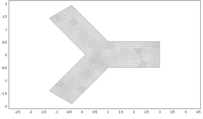
specified. Species concentration is not known at the boundary and an approximation regarding species diffusion, the only term that connects the species field within the domain to the species distribution on the outflow boundary, is required. The potential conditions are selected so that fully developed electrokinetic flow occurs across the inlet faces (left side) and outlet face (right side) in Figure 1. The top branch has twice the potential at the inlet to the bottom branch, relative to ground taken six lengths downstream from the outlet. The exact set up of the electrokinetic flow network model for which this junction is the key element is given in Zimmerman (2006).

The electric field is taken as quasi-steady, that is the electric field adjusts practically instantly to changes in the velocity and concentration. The above equations represent a generic problem providing a test of the numerical implementation which when verified may allow computation of any particular electrokinetic flow conditions. For the study here, we take the

same indicative coefficient values as Zimmerman (2006): 1 Re = 30, 1/ Pe = 0.03, �_r = 1 (no

variation in wall zeta potential), z= 0 (no charge on species Y) and �_r = 1 (no variation in

electrical conductivity).

The special focus of this case study is the role of reaction R in the species transport, Eq. (3). In these scalings, R for a quadratic takes the form:

R� �Da Y

�

1�Y

�

(6)

where Da is the Damkohler number, a dimensionless reaction rate. We have particularly selected a nonlinear reaction as to distinguish the influence of the Damkohler number from the linear processes in Eq (3): convection and diffusion. The elementary reaction that is consistent with Eq (6) is isomerization of a solute molecule into a solvent molecule, which is not particularly of practical importance. It is one of the simplest nonlinear reaction schemes to consider, however, as it only requires monitoring of one species, and is thus taken as an exemplar here.

§2.2 Forward problem

The forward problem is the classically stated one: given the PDE system Eqs (1)-(6) and appropriate boundary and initial conditions (described in the network model by Zimmerman (2006)), and the physical parameters expressed here as their dimensionless counterparts, the Peclet and Damkohler numbers, can we predict the output concentration profile throughout

all time? Indeed, can we predict all the field variables: �, u,v,p, Y?

Since there is no general analytic solution to such a multiphysics model with complex boundary and initial conditions, we typically resort to numerical approximation schemes. Here we follow Zimmerman (2006) in adopting the Galerkin finite element expansion method on the mesh plotted and described in Figure 1. The model is implemented in Comsol Multiphysics 3.3 with standard application modes for the Navier-Stokes equations (Lagrange P2-P1 elements for velocity and pressure), DC conductive media, and convection/diffusion, both with second order Lagrange polynomial basis functions. The discretization is fairly coarse, with up to 2% approximation error. Given the large number of model evaluations, this represents a trade-off of accuracy for computational time usage.

Figure 2 shows the pseudo-steady operation achieved after t=3 where the whole channel is

channel due to double the electric field strength of the lower channel. This pseudo-steady operation always has a modest feed of solute through the lower channel and a much stronger feed of solvent through the upper channel. Switching the voltages achieves a “slug” formation of solute-solvent-solute etc. in the channel.

In order to visualize the dynamics of this slug formation, we define a global measure

0.5

Y t

� �

�

�

Y x

�

�3, ; y t d

�

t

�0.5

for which the time series evolution is shown in Figure 3.

[image:9.595.98.497.260.495.2]

Figure 2 Electrokinetic reactor condition after t=3. The arrows are the induced, steady state velocity field from the electroosmotic flow. The contours are equi-potential lines for the electric voltage. The shading represents concentration of solute. Clearly a region of high solute concentration has been bypassed by the flow from the upper channel through the Y-junction switch.

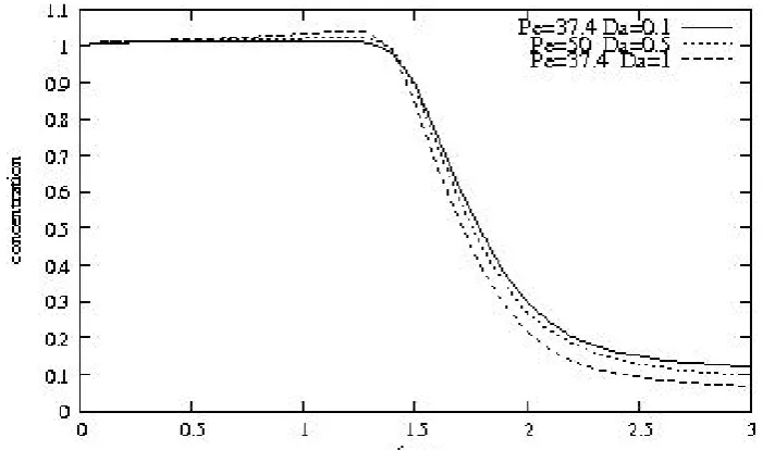
There are three parametric studies shown in Figure 3. Variation of Pe and Da achieves little difference in the qualitative structure of the system response. The decline rate changes modestly and the plateau level are also somewhat affected by these parameters. Visually, variation of either parameter would seem to act in opposing directions so that qualitatively, changing one parameter looks much like changing the other in the opposite sense. If the equation system were linear, then the overall transfer function could not discriminate between such parameters. However, since the reaction term in Eq. (8) is nonlinear, these two

parameters must have different dependencies. Whether the output measure Y t

� �

is sensitive

[image:10.595.100.497.108.347.2]

Figure 3 Output average concentration of solute (averaged along the x=3 face in Figure 1) vs. time for 0<t<3 with three cases from low (Da=0.1, Pe=37.4) to high (Da=1, Pe=37.4) Damkohler numbers, but with an intermediate case of (Da=0.5, Pe=50). This intermediate case was deliberately selected to show that in this model, varying Damkohler numbers and varying Peclet numbers have visually indistinguishable response. One could seemingly see the same profile by varying either parameter independently. Note that the modest rise at early times in concentration is an artefact of the discretization error, which can be as large as 2% with the coarse mesh used in Figure 1.

Convergence studies and error estimation.

Table 1 shows the degrees of freedom used in the typical resolution mesh of Figure 1 (with 3840 elements and 34481 degrees of freedom), and both in lesser and greater grid resolution for the particular case of Pe=40; Da=0.3, selected as an exemplar for the speed of calculation and error estimation of the outflow average profile history of 31 data points in the interval of

t�[0,3]. The zero-norm, i.e. the maximum discrepancy between different levels of mesh

[image:11.595.87.438.84.291.2]

resolution, does not diminish substantially with finer mesh. That the average concentration at the outlet is smaller than the point-wise error is not unexpected, but the slow convergence might seem odd. It is actually intrinsic to the electrokinetic flow model including sharp corners or walls with high curvature. The corner is a singularity of the electric field and induces a singular velocity – the convergence of the model becomes slower in CPU time in treating this numerical artefact. Craven et al. (2008) demonstrates a boundary layer correction to the corner region that can improve the convergence and accuracy by solving the Poisson-Boltzmann equation in the near corner region. However, the error estimates of within half a percent for the maximum discrepancy are sufficient for most engineering purposes.

Table 1

Index n DoF Max discrepancy

� �_{� �} � 1 �_{� �}

0

n n

c t �c � t

CPU time (s)

0 2504 --- 32

1 9083 0.0064 66

2 34481 0.0092 414

[image:11.595.86.547.637.733.2]

§2.3 Inverse problem and parametric sensitivity

Parametric sensitivity and inverse methods have as a basis, the inverse function theorem of

vector calculus. If the classical forward problem is the prediction of measurable outputs

from the selected operating conditions and physical parameters, the inverse problem is the estimation of the physical parameters from the measured outputs as the performance of a

system under known operation conditions. Let’s introduce the notation that all the

operational parameters are a vector

�, the kinetics parameters are a vector

k , and the

measurements are a vector m . Then the predictive model is, generically,

m �f

�

k��

�

(7)

The inverse function theorem tells us that it is possible to define locally an inverse function

k �f �1

�

m��

�

(8)

only if the Jacobian of the transformation is non-singular, i.e. det

�

J

�

�0

�f (9)

J � i ij _�

k_j

This is equivalent to the Hadamard (1923) criteria. An inverse problem is described as well posed if:

1. The solution exists for any data, k , in the dataset.

2. The solution is unique in the image (measurement) space.

3. The inverse mapping, m �k , is continuous.

Numerically, it is extremely rare for a Jacobian to be exactly singular, due to round-off errors. Thus, instead, the degree to which a matrix is singular is assessed by its condition

number. The condition number for J is found by conducting its singular value

decomposition (SVD) (see Golub and Van Loan, 1996) to find its list of singular values

s₁ �…s _n , if J is an n n� matrix. The condition number is found from the singular values with

max �si�

the maximum and minimum magnitude N_c � _{min �s}

i� . Since a singular matrix has at least one

zero singular value, n_c � �. In practice, nearly singular systems have high condition

numbers. A rule of thumb has developed with condition numbers which suggests that

log ₁₀ N_c represents the number of significant digits of information that are lost in the matrix

inversion. This gives an indication of the best sensitivity expected of the inverse problem, no matter how the inverse function (8) is estimated.

Essential to the above argument of invertibility and sensitivity is the selection of output

performance measures m . Typically, output measures are imposed practically, limited by

These days, it is possible to collect an enormous number of different measurements m , but the inverse function theorem only applies to square Jacobians – where the number of

unknown parameters k and the number of measured outputs are equal. This would suggest

that we can only use the inverse function theorem and the condition number criterion when we limit ourselves to the same number of measurements as unknown parameters, but this

could be throwing away valuable information, particularly if we do not know, a priori, which

measurements are likely to be informative. For instance, in Figure 3, there are thirty-one

output average concentration measurements embedded in the graph for time intervals �t=0.1.

Since there are only two physical (kinetic) parameters in the problem (Da and Pe), which two time points would make the best representation of the experiment?

In such cases, it is useful to select derived or summary measures that are more informative

than any single pointwise measurement. Zimmerman (2005a,2006a,b) used Fourier

transform coefficients as derived measures representative of time series of irregular

oscillations. Jeanmeure et al. (2002) in a multiphase flow sensing application used

symmetric and antisymmetric combinations of electrical capacitance sensor readings as global measures. More prosaically, Bandulasena et al. (2008abcd) use spatial and statistical moments of temperature and pressure as global measurement factors. Even then, however, it may not be possible to find a set of measures for which the number of measures equals the number of unknown parameters and the mapping is invertible with a well-conditioned Jacobian matrix, Eq (9). For instance, Zimmerman et al. (2006) show that the two parameter Carreau constitutive model of a non-Newtonian fluid undergoing electrokinetic flow cannot be estimated by fewer than three pressure moments. Those authors demonstrated a pseudo-invertible 2-D manifold in the 3-D space of the first three pressure moments of a wall-embedded pressure sensor were sufficient for parametric estimation.

Regression, least squares fit, and pseudo-inversion are related concepts for how to estimate a

set of fewer unknowns than collected measurements. We propose here that if the

measurement system (7) is overdetermined (more measurements than parameters), then the appropriate analogue of the Jacobian for for estimating the sensitvity to inversion is the Gramian matrix, defined as

T

G �J J (10)

This can be seen by writing the Taylor-Series expansion of (11) around the measurement point (k₀ �m₀) :

m �f

�

k0 ��

�

�J

�

k �k0

�

(11)

which can be re-written more suggestively as:

�m �J�k (12)

It follows that the parameters k can be determined by the pseudo-inverse of (11):

�k �G�1JT�m (13)

It follows that the same argument for the sensitivity of the invertibility of the square Jacobian follows in the non-square case for the Gramian – the condition number of the Gramian tells of the relative sensitivity of the pseudo-inversion process.

Additionally, the argument above is constructive for the pseudo-inversion if the function f

is known by table lookup:

� Find the element in the table closest to the measurements m . Call this point

k ₀�m ₀ .

� Estimate the Jacobian J from the finite difference formula from nearby

m �m J _ij � i 0�i

k_j �k_0�j

� Compute �k according to the formula (13)

This approach is somewhat different from classical regression analysis, which minimizes the squared error by requiring stationarity to produce the normal equations.

Table lookup (or mapping) is a good approach if the dimensionality of the problem is sufficiently small that populating the table is not too expensive. If computing the forward map is cheap, it can also be quick to find the pseudo-inverse by optimization techniques. We

are looking to minimize the error of the predicted measurements m with the actual

measurements, which can be restated as minimizing the error estimate E:

2

N �_m measured �_m predicted �

n n

E�

�

w e _{n n} , e _n � �_�

mscale �� (14)

n�1 � �

m

If the weights w_n �1 and the scales mscale _�

1, then this is called the least squares regression, i.e.

m

min E (15)

k

specifies the best estimated set of physical (kinetics) parameters k from the measures m .

If the predictions m �f

�

k��

�

can be specified analytically in closed form, then the normal

equations that require stationarity of Emay be formulated in a simple, closed form, which is

the case for nonlinear regression. Solving the typically nonlinear normal equations, however, may not be particularly straightforward, however. One robust approach to finding the

minimum E (15), is the Nelder-Mead algorithm [Nelder and Mead (1965)], which shrinks a

simplex region until convergence around a (possible local) minimum occurs.

Let’s define the vector m as the 31 values of

m _n �Y t

� �

_n

t _n �

�

n�1

�

�t

with �t=0.1. The functional form of

m = f

�

k,�

�

k �

�

Pe,Da

�

and with � the operating parameters (induced Reynolds number from voltages) is not known

in closed form, but is well posed algorithmically as the numerical estimation of Y t

�

_n

�

by

Galerkin finite element methods: the forward problem of §2.2. Similarly, E in Eq. (15)

cannot be computed readily or usefully in closed form, but it can be approximated easily to great accuracy.

The algorithm for optimisation of (15) follows this general outline:

measured

1. Select a guess of Peand Dawith target data m ,

2. Compute the FEM solution to Eq. (1)-(6) and (8).

3. Use (�, u,v,p, Y) approximations to compute mpredicted �Y t

�

_n

�

4. Use mpredicted to calculate Eby Eq. (15).

5. If E is not minimal, then select a new guess for Pe and Da according to a directed

search algorithm.

FEM solution is packaged as a function that is fed to the optimization algorithm. Substantial speed up can be found by computing the numerical solution to the FEM model simultaneously to optimizing the target function by using the Newton iteration algorithm for an error estimate that includes the estimation of the PDE approximation error (FEM model)

and target function E. The Newton iteration algorithm also selects the next parametric guess

for k �

�

Pe,Da

�

. This has the disadvantage that the search is not modular and must start sufficiently close to the minimum so that the Newton iteration is well conditioned.

Figure 4 General decrease in estimation error by the Nelder-M ead algorithm over an epoch of 90

-4

iterations to less than the target tolerance of 10 . The approach to this error tolerance level for the lastest thirty iterates is extremely slow, but that reflects the fact that the PDE engine for the forward

-4

problem was also set to a global convergence tolerance of 10 . For the inverse method to converge faster requires a finer mesh than Figure 1 and a tigher convergence criteria.

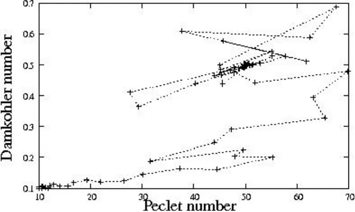
Figure 5 Trajectory followed by the Nelder-M ead algorithm in approaching the minimum error in Peclet-Damkohler phase space for the target output performance shown in Figure 3 for Pe=50 and Da=0.5. M ost of the iteration time is spent meandering around the final optimum.

Figure 4 shows the error E at each iterate of the Nelder-Mead algorithm over an epoch of 90

-4

[image:15.595.88.442.202.412.2] [image:15.595.90.444.483.694.2]

guesses of k �

�

Pe,Da

�

take following the Nelder-Mead algorithm implemented in Matlab

from the initial guess of k₀ �

�

Pe �10, Da �0.1

�

for the target data of

k_� �

�

Pe �50, Da �0.5

�

shown in Figure 3. Different initial conditions eventually converge

[image:16.595.120.486.201.491.2]

on the same target data, consistent with a unique optimum. The condition number analysis in Figure 6 actually confirms the uniqueness of the inversion in this parameter range.

Figure 6 Condition number analysis of the Gramian matrix for the forward model of an electrokinetic reactor. In general, the conclusion is that inversion for low Peclet number and high Damkohler number is easier to achieve as the surface slopes downward in that direction. The “pits” in the surface represent particularly identifiable parameter regions. In general, lower condition number leads to higher parametric sensitivity and thus more informative regions for experimentation. The fact that the log(condition number) is low in this range of Peclet numbers shows that the pseudo-inverse problem is well-conditioned and unique within this range.

Figure 6 shows the condition number analysis of the Gramian matrix (10). Since the 1

log ₁₀

�

N_c

�

_�2 �4 , the Gramian is far from singular. Consequently, every k �

�

Pe,Da

�

2

pair in the range shown in Figure 6 is pseudo-invertible. The surface declines towards the high Damkohler number and low Peclet number range, indicating that this region is more readily invertible. As the Da is intrinsic to the fluid, reaction system, and geometry, it is not possible to change it by different operating conditions with the same experimental set up. The Peclet number, however, does vary with superficial velocity so it can be varied by

changing the operating voltages which induce electroosmotic flow. Consequently,

decreasing the imposed voltage will generally improve the parameter estimation for both

� �

In general parametric scanning can be used to find the best operating conditions for

experiments to optimally estimate the kinetic parameters k �

�

Pe,Da

�

by varying the

experimental conditions �. Zimmerman (2006a,b) followed the prescription of Varma et al.

(1999) which seeks the highest sensitivity value for a given measurement component mn as

the best operating condition. Zimmerman (2005) found that high susceptibility to inversion occurred under resonant conditions in forced oscillations, consistent with the findings of Zimmerman (2006a,b) that the greatest susceptibility to inversion occurs with the highest

nonlinear response in forced oscillations. In the next subsection, we present a dimensionless

sensitivity method for parameter scanning to find the region of greatest sensitivity for

inversion for a single parameter kn. The lowest condition number region of the Gramian

matrix (or the Jacobian if square) is the region of best susceptibility to inversion for all parameters, but does not single out any particular parameter. It also has the potential to be a dimensional quantity if the problem statement is not non-dimensionalized as here. Consequently, it is only a relative measure of (pseudo)-invertibility.

§2.4 Parametric sensitivity, parameter scanning and optimal experimentation

Canonically, we represent the kinetics of a dynamic system in terms of the rate of change of the concentrations of a set of unknowns (sometimes termed degrees of freedom) which in the

FEM approximation are the Galerkin coefficients, ci(t). Such a system can be represented

functionally as a system of typically nonlinear ODEs in time:

dc_{i �}

F_i

�

c, ; t k;�

�

(16)

dt

We identify global measures that summarise the system response as

m �G

�

c

�

0 ;

�

� �;

�

�G

�

�

�

t

�

�

(17)

where G is a function of the system parameters that can be controlled externally, and a

functional of the time series of concentrations. Not that G is not a dynamic quantity – it is independent of time and representative of the whole time series. The inverse problem is to

estimate best k to fit the experimental measures gl from lsets of operating conditions �l.

m_l �G

�

c

�

0 ;

�

�_l;�

�

(3)

Recall that our error E in Eq. (14) is computed from contributions from each measure:

e_l �e_l

�

c

�

0 ;

�

�l;�

�

(5)

For a fixed experimental data set, that is ci(0) and �l held constant, the normalized error

contributions em are only dependent on the kinetics parameters k in the model. Thus, the

most sensitive parameters are those that induce the greatest change in the error measures el.

Around any current estimate of the model kj, a Taylor series expansion of an arbitrary

variation of by �kj yields this expression to linear order:

�

k

�

�

e k

� �

�

H

�

(6)

e k

l j

� �

j l j lj j

where

�e �kj ₍₇₎

H �k l

lj j _� j

k_j k_j

and there is no summation over the index j.

The matrix H is dimensionless. The vector � quantifies the fractional variation in the

kinetics parameters and is also dimensionless. The element of H which has greatest

the new experiments) on improving. Similarly, the evolving model can be used to scan the

space of operating conditions �l to determine for a given target kinetics parameter, which

experimental conditions will give it greatest sensitivity.

Clearly with regards to the electrokinetic flow reactor, since the “experimental” data is simulated, this is not a true test of the methodology. Should the reader be concerned that such inverse methods only work with simulated data, not real experimental data, she is referred to Deshpande and Zimmerman (2005a,b) which demonstrates parameter identification of both mass transfer coefficients in a two phase binary reacting system from experimental data. Zimmerman (2005a) reviews the use of parameter identification in chemical engineering and systems biology. Recent examples of parameter identification in systems biology include proximate parameter tuning using linear programming for biochemical networks and translation initiation (Wilkinson et al., 2008; Dimelow and Wilkinson, 2009). A general framework optimising Fisher information for integrating experimental design and parameter identification in the face of uncertainty has recently been developed (Chu and Hahn, 2008) which is also potentially applicable to PDE modelling.

§3 Conclusions and recommendations

We have presented a critical analysis of the current state of the art in microfluidic microchip technology aimed at the question of why microfluidic chemical technology microfluidic sensors lag behind biotech/biochem applications, with still no mass production of onchip microreactors or microfluidic sensors. The analysis suggests that the unique advantages to biotech/biochem assays available through micro-TAS systems and similar devices found immediate application in biotechnology as they represented capability that was not otherwise possible, and were not particularly hampered by the bane of microfluidic technology – overcoming the micro/macro interface problem.

We also discussed three developing technologies from our own research – microbubble generation, microfluidic plasma reactors, and microfluidic rheometry. All three are aimed at exploiting advantages of microscale processes not present in conventional scale counterparts and have solutions to the micro/macro interface problem that may be at best a positive benefit for creating the product at the microscale due to using microbubble “packaging”. At worst case, the microrheometric sensor is only producing “information” so if used for online monitoring, it could discard the small samples taken if reinjection into the process stream is problematic.

We also extrapolate the current trend of our own work which could become the new paradigm for microfluidic chemical technology design and development work:

1. Multiphysics models are now cheap to develop and in the case of transport in microchannels, highly accurate.

2. Inverse methods can be modularly developed for the estimation of physical and kinetics parameters of the multiphysics models from performance data of the device, therefore eliminating the need for reductionist methods for parameter measurement. This is especially important with only small samples of fluids to manipulate.

until a sufficiently predictive model is developed for either design or control purposes.

This paper illustrates all three elements of the paradigm with regard to either the electrokinetic flow reactor example (points 1 and 2) and the microfluidic rheometer (all three points). Elements of the paradigm (point 1) were important in the development of the ozone plasma microreactor and are forecast to be of greater importance in more general onchip plasma reactions.

As microfluidics bodes to improve the sustainability of chemical processes in the future, this article contributes to the roadmap the recommendation that greater effort and resources go into expanding the use of the paradigm for optimal modelling and experimentation, in particular into exploring the development of multiphysics inverse methods in microfluidic design.

Acknowledgements

WZ would like to thank support from the EPSRC for the development of the acoustic actuated fluidic oscillator (Grant No. GR/S67845) and for financial support from the Food Processing Faraday Partnership, Yorkshire Water, and Sheffield University Enterprises Ltd. Additional support from EPSRC GR/S83746 for the microrheometry, EP/D004748/1 for the plasma microreactor, and EP/D031311/1 for the modelling and inverse methods are acknowledged. WZ would like to thank the Royal Academy of Engineering / Leverhulme Trust Senior Research Fellow programme. The authors would like to acknowledge support from EP/E01867X/1 (Bridging the Gap between Mathematics, ICT

and Engineering Research at Sheffield). The authors thank Ray Allen, Hemaka

Bandulasena, Mark Bown, Tom Craven, Buddhi Hewakandamby, Jaime Lozano Parada, Laurent Jeanmeure, Jordan MacInnes, Peter Styring, and Vaclav Tesar for helpful discussions.

References

Bandalusena H C H, W B Zimmerman and J M Rees “An inverse methodology for the rheology of a power law non-Newtonian fluid.”J Mech. Eng. Sci.222(5):761-768, 2008a.

Bandalusena H C H, W B Zimmerman and J M Rees (submitted 2008b) Microfluidic rheometry of a polymer solution by micron resolution particle image velocimetry: Model validation and Inverse methodology. Submitted to Journal of Rheology.

Bequette BW, Process Control: Modeling, Design and Simulation, Prentice Hall (2003).

Bown MR, MacInnes JM, Allen RWK, Zimmerman WBJ, “ Three-dimensional, three-component velocity measurements using stereoscopic micro-PIV and PTV”, Meas. Sci. Technol.172175-2185, 2006.

Broadwell, I., P. D. I. Fletcher, S. J. Haswell, X. Zhang, R. W. K. Allen, J. M. MacInnes, “Pressure-Driven and Electroosmotic Flows and Electrical Currents in Lab-on-a-Chip Micro Reactor Devices” Trends in Physical Chemistry10, 117-133, 2004.

Chen BH, Asprey SP On the design of optimally informative dynamic experiments for model discrimination in multiresponse nonlinear situations. Ind. Eng. Chem. Res. 42 (7): 1379-1390, 2003.

Chu YF and Hahn J, “Integrating parameter selection with experimental design under uncertainty for nonlinear dynamic systems,”AICHE J. 54 (9): 2310-2320, 2008.

Chen L. , Manz A , Day PJR “Total nucleic acid analysis integrated on microfluidic devices.” Lab Chip. 7 (11):1413-1423 17960265, (2007) .

Craven T J, J M Rees and W B Zimmerman On pressure sensor positioning in an electrokinetic micro-rheometer device. Part I: Simulation of shear-thinning liquid flows. To be submitted to Journal of Microelectromechanical Systems.

Craven T J, J M Rees and W B Zimmerman, “On slip flow velocity boundary conditions for electroosmotic flow near sharp corners.” Physics of Fluids. 20:043603, 2008. co-Published in the American Institute of Physics Virtual Journal of Nanoscience, 5 May 2008.

de Mello AJ and Beard N, “Dealing with real samples: sample pre-treatment in microfluidic systems, Lab. Chip 3:11N--19N, 2003.

Deshpande K.B. and W.B. Zimmerman, ``Experimental study of mass transfer limited reaction.

Part I: A novel approach to infer asymmetric mass transfer coefficients’’ Chemical Engineering Science

60(11)2879-2893, 2005a.

Deshpande K.B. and W.B. Zimmerman, ``Experimental study of mass transfer limited reaction. Part II: Existence of crossover phenomenon.’’Chemical Engineering Science60(15) 4147-4156, 2005b.

Dimelow RJ and Wilkinson SJ, “Control of translation initiation: a model-based

analysis from limited experimental data”J. R. Soc. Interface(2009) 6, 51–62, doi:10.1098/rsif.2008.0221 Golub G.H. and Van Loan C.F. “Matrix computations'”. 3rd ed., Johns Hopkins University Press, Baltimore, 1996.

Hadamard, J. Lectures on the Cauchy problem in linear partial differential equations. Yale University Press, New Haven, 1923.

Hu S, “Novel bubble aerator performance,” University of Sheffield, MSc in Environmental and Energy Engineering dissertation, 2006.

Jeanmeure LFC, T.Dyakowski, W. B. J. Zimmerman and W. Clark ``Direct flow-pattern identification using electrical capacitance tomography,’’ Experimental Thermal and Fluid Science 26 (6-7): 763-773, 2002. Lane S., E. B. Martin, A. J. Morris, P. Gower. Application of exponentially weighted principal component analysis for the monitoring of a polymer film manufacturing process. Transactions of the Institute of Measurement and Control 25(1), 17-35, 2003.

Lieberman M.A. , A.J. Lichtenberg, Principles of Plasma Discharges and Materials Processing, 2nd ed., John Wiley and Sons, 2005.

Lozano Parada JH, “Microchannel plasma reactor development”, PhD thesis, University of Sheffield, 2007. MacInnes J. M., “Computation of Reacting Electrokinetic Flow in Microchannel Geometries”, Chemical Engineering Science, 57 (21), 4539-4558 (2002).

MacInnes, J. M., X. Du and R. W. K. Allen, “Prediction of Electrokinetic and Pressure Flow in a Microchannel T-junction Physics of Fluids15(7), 1992-2005, 2003.

Nelder J. A. and Mead R. “A simplex method for function minimization.” Computer Journal, 7:308-313, 1965.

Pieroziello G., “Packaging of microfluidic systems: a microfluidic motherboard integrating fluidic and optical connections” PhD thesis, Technical University of Denmark, 2006.

Stone VN , Baldock SJ, Croasdell LA, Dillon LA, Fielden PR, Goddard NJ, Thomas CLP,

Treves Brown BJ, “Free flow isotachophoresis in an injection moulded miniaturised separation chamber with integrated electrodes”. J Chromatogr A. 17229431, 2006.

�����V, Zimmerman WBJ, “Aerator with fluidic oscillator,” UK0621561, 2006.

Varma A., Morbidelli M., Wu H. Parametric sensitivity in chemical systems, Cambridge Series in Chemical Engineering, Cambridge University Press, 1999.

Wilkinson, S. J., Benson, N. and Kell, D. B. Proximate parameter tuning for biochemical networks with uncertain kinetic parameters. Mol. Biosyst.4, 74-97 (doi:10.1039/ b707506e), 2008.

Zimmerman WBJ (ed.), Microfluidics: History,Theory, and Applications, Springer-Verlag-Wien, CISM Lecture Series, No 466, Berlin, 2005.

Zimmerman W.B., “Metabolic pathways reconstruction by frequency and amplitude response to forced gylcolytic oscillations in yeast. “Biotech. Bioeng., 92(1): 91-116, 2005a.

Zimmerman WBJ, Multiphysics Modelling with Finite Element Methods, World Scientific Series on Stability, Vibration and Control of Systems, Vol. 18, Singapore, 2006.

Zimmerman W.B., “Role of helicity on the quality of microchannel plasma generation” Final Report, EPSRC EP/D004748/1, 2007.

Zimmerman W.B., “Cheating Nyquist: nonlinear model reconstruction with undersampled frequency response of a forced, damped, nonlinear oscillator.” Chemical Engineering Science, 61:621--632, 2006a.

Zimmerman W.B., “Nonlinear model reconstruction by frequency and amplitude response for a heterogeneous binary reaction in a chemostat.” Chemical Engineering Science, 61:605— 620, 2006b.

Zimmerman W.B.J., J.M. Rees, and T.J. Craven, “Inverse problems in non-Newtonian electrokinetic flows in microchannel networks,” ESDA Manchester ASME Transactions, 2004.

Zimmerman, WB J.M. Rees, and T.J. Craven, “Rheometry of non-Newtonian electrokinetic flow in a microchannel T-junction,” Microfluid. Nanofluid 2:481— 492, 2006.