Using computer software packages to enhance the teaching in Engineering Management Science: Part 3 - Simulation
H Ku and R Fulcher
Faculty of Engineering and Surveying, University of Southern Queensland, West Street, Toowoomba, Queensland 4350, Australia.
Ku, H and Fulcher, R., Using computer software packages to enhance the teaching of Engineering Management Science: Part 3- Simulation, Journal of Computer Applications in Engineering Education, 2010, DOI: 10.1002/cae.20423 (published online).
Corresponding Author: Title : Dr.
Name : Harry Siu-lung Ku
Affiliation : Faculty of Engineering and Surveying, University of Southern Queensland. Tel. No. : (07) 46 31-2919
Fax. No. : (07) 4631-2526 E-mail : [email protected]
Abstract
This paper is the third paper in a series of sharing the experience of using different software
packages in the delivery of Engineering Management Science coded as ENG4004, in the Bachelor of Engineering and Bachelor of Engineering Technology programs offered by the
University of Southern Queensland. The paper describes how the authors use different
software packages to solve the simulation problems of the course, using Monte Carlo
technique. Sometimes more than one package is required for the effective delivery of a topic
of the course. The needs for the usage were also explained. The assessments of the course
were also studied and reviewed. How the software packages met the objectives of the
module were also discussed together with the desired learning outcomes of students. The
preferred software was Excel in MS Office. It can be argued that the students‟ learning
experience and satisfaction will be greatly increased with the software packages while the
cost to the university will be minimal.
Keywords: engineering management science, Quantitative Methods – Production and Operations Management (POM-QM) for Windows 3, Excel in Microsoft Office, simulation
and Monte Carlo technique.
Introduction
The application of computers in engineering education is now much more than simply
teaching students to use programming languages, e.g. C++. It also teaches how to use certain
software packages to solve the problems in their course. Computer and its related software
USQ, Engineering Management Science (EMS) is offered as the core course to seven engineering degree programs, ranging from building and construction management to
mechatronic engineering. It is a one-semester course and is offered in semester two (2) every
year and semester three (3) in alternate years. In addition, the course is offered as
face-to-face on-campus study as well as print based delivery, in which studybooks and other
materials, e.g. CD-ROM are mailed to students worldwide. Additional support given to
off-campus students includes communication by telephone, e-mails and Moodle (web-based
computer technology) through the Internet [2]. For the on-campus study, the course is
currently available only at Toowoomba campus (Other campuses are in Fraser Coast and
Springfield). Today, Engineering Management Science software packages have been mainly developed by software companies and individuals who have ample knowledge about the
subject [3]. In USQ, the course is delivered to both on-campus and off-campus students and
this adds to the challenge of delivering the course successfully.
There are five parts in the series of these articles: the first one is the use of software packages
in delivering critical path networks; the second is the application of software packages in
programming techniques: distribution method and simplex method; the third is the utilization
of software packages in delivering simulation using Monte Carlo technique; the fourth is the
utilization of software packages in delivering quality control and the last is the use of
software packages to deliver financial analysis: break even analysis and net present value.
The topics covered in five parts constitute the modules in the course, Engineering Management Science.
This paper is the third one in the series and covers the application of software packages in
simulation using Monte Carlo technique. Unlike the previous paper of the same series, the
2007 (MS Office 2007) and Quantitative Methods – Production and Operations Management (POM-QM) for Windows 3 written by Howard J Weiss [4]. This will cost the university even less than the previous case, the use of software packages in delivering critical
path networks.
Courseware and software package
The present courseware of Engineering Management Science (EMS), ENG4004 consists of five topics which are critical path networks, programming techniques, simulation, quality
control and micro-economic functions. In the past, the course has been offered without using
any software packages. Students were taught the theories of different topics in EMS and were
then asked to solve simple problems manually but enrichment to the course is now necessary.
One enrichment necessary is the additional use of software packages, like Microsoft Quantitative Methods – Production and Operations Management (POM-QM) for Windows 3
for the second topic, Critical Path Networks [5]. If these were absent, people might think that the course is out of date as most engineering science management textbooks include
them. The next question is how to select a package that suits the remaining 3 topics in
ENG4004 at USQ. Turban and Erikson [3] discussed the selection of engineering
management science software for PCs in detail. The first step of the selection process is
defining the problem. The second module of the course, ENG 4004 is Programming Techniques and Keytack [6] mentioned that several textbooks had started to include a software package that deals with most of the decision science problems as early as 1994.
Simulation packages
The simulation discussed in the studybook is Monte Carlo technique. In most textbooks including the one for the course, the variable in the simulation problems is only one and
hence only one set of random numbers will do the job. In the course, the simulation
problems have two sets of interdependent variables. This makes the problem more difficult
but realistic.
Consider an example in the study book in which a product passes two processes A and B in
that order. The processes are connected by a conveyor and the partly processed component
takes a fixed time of 0.05 minutes to travel down the conveyor from process A to process B.
The average time for process A is 0.55 minutes and for process B is 0.51 minutes for each
component. It is desirable to know the average number of components that are expected to
queue up between A and B as well as the average output of the process line. The distribution
of the processing times for A and B are given in Figure 1 (left hand side for A).
This simulation problem cannot be solved using POM-QM for Windows 3 because the package can only be used to solve simulation problem with one variable only. The better
option will be Excel in MS Office 2007 as this spreadsheet software can be used to solve simulations quickly [7].
The processes of inputting the information to the spreadsheet are as follows:
1. Enter probability distributions for Processes A and B in Figure 1; a set of cumulative probability values are entered in „column B‟ for process A. These cumulative probabilities
are done by first entering 0 in cell B4, then entering “=A4+B4” in cell B5, copy
this formula into B6:B16. Figure 2 shows the entries for the simulation for Processes A and
2. Enter “=RND()” into cell B21 to generate random number for process A. Copy B21 into
B22 to B40 for 20 simulations.
Process times for Process A were generated by each of these random numbers in B21:B40.
This is accomplished by first covering the cumulative probabilities and the process times in
cells B4:C16 with the cursor. Give this range of cells the name “process_A”
3. Enter “=VLOOKUP(B21, process_A,2)” into cell C21 and copy it to cells C22:C40. This
formula will compare the random numbers in „column B‟ with the cumulative probabilities in
B4:B16 and generate the correct time from cells C4:C16. Once the times for Process A have
been generated in „column C‟, the times for items ready for Process B can be determined.
4. To generate times for items ready for Process B, enter “=C21” into cell F21. Enter “=F21” into cell G21 and copy it to cells F23:F40. Enter “=G21+E21” into cell H21The input is
ready for item 1 only. For other items, the procedures are carried out after performing the
procedures times for Process B is done in step 5.
5. Repeat the procedures of 2 and 3 for Process B. Once the times for Process B have been
generated in column D, the times for Process B to begin can be determined.
For item 2 onwards, enter “=(MAX(F22,H21))” into cell G22 and copy G22 to cells
G23:G40. Enter “=F21+C22” in cell F22 and copy it to cells F23:F40. Copy H21 to cells
H22:H40. Copy H21 to cell G23:G40.
6. Enter “=C21” into cell I21 for Process B idle time for item 1. For items 2 and onwards,
7. Enter “=(-MIN(F21-G21,0))” into cell J21 for waiting time of the first arrived but need
waiting item from Process A to Process B. Copy J21 into cells J22:J40.
8. Enter “=MAX(H21-F23,0)” into cell K21 for waiting time of the second arrived but need
waiting item from Process A to Process B. Copy K21 into cells J22:J38.
9. Enter “=IF(J21>0,1,0)” into cell L21” and copy it to L22:L39 to check whether there is
item 1 waiting.
10. Enter “=IF(K21>0,1,0)” into cell K21” and copy it to K22:K38 to check whether there is
item 2 waiting.
11. Enter “=SUM(I21:I40)” into cell B43 to evaluate total idle time for Process B.
12. Enter “=(SUM(J21:J40)+SUM(K21:K40)) into cell E44 to evaluate total waiting time for
components.
13. Enter “=(20*60)/(SUM(C21:C40))” into cell G43 to evaluate average production of A.
14. Enter “=(20*60)/(H40-B43)” into cell J43 to evaluate average production of B.
15. Enter “=(20*60)/(11.7)” into cell B46 to evaluate average production of A + B.
16. Enter “=E44/10.65” into cell H46 to evaluate average number of components waiting
It can be found that the process is quite long and tedious but the programming is reasonable
for engineering students. For simulation problems with more than two variables, Excelin MS Office 2007 can be used to solve them but it will be even more tedious and complicated. On the other hand, for problems with one variable, Excelin MS Office 2007 can solve them with ease and POM-QM for Windows 3 can solve them even easier because there is no programming at all with the second package. For the simulation problems in ENG 4004,
Engineering Management Science, the authors would like their students to use Excel in MS Office 2007 to solve the simulation problems as the other package cannot solve these problems, as it is limited to one variable only.
Assessments
At the moment, there were three assessments for the course, two assignments and one
examination. Starting from semester two (2), 2008, the first assignment will deal with critical
path network analysis with a weight of 15 %; the other one will be for distribution method or
simplex method (programming techniques), simulation and control charts (quality control)
respectively with a weight of 25%. Suggested solutions with marking schemes were sent to
students via Moodle on the due date of each assignment and no extension of assignments was
permitted. External students handed in their assignments by mail via the USQ Distance and
e-Learning Centre and were returned to them via the same pathway. Students are expected to
spend about four hours on each assignment. The last assessment is a 2-hour open book
examination which consists of five questions and contributes to 60% of the total marks. The
first question is a compulsory question based on critical path networks and contributes 150 of the totals marks of the course. The other four questions covered the remainder of the topics;
students were required to attempt any three of them; each contributes 150 of the total marks
In this paper, only part of the second assignment – simulation will be discussed. The
simulation question of assignment 2, semester two (2), 2009 describes that the Butah Coal
Mining Company wishing to establish a coal dumping area beside a larger conveyor used to
transfer coal to ships anchored periodically in an adjacent harbour. Coal is transported by
truck from a coalfield some distance away and before dumping the coal is weighed.
Processing at the weighing and dumping facilities varies between one and ten minutes and a
sample taken over 200 trips (see Table 1) show the distribution of processing times.
Students will be required to simulate the weighing and dumping of coal from eight trucks (i)
manually and (ii) using Excel. For (i), use the random numbers provided in Table 2. Based
on this analysis, construct the cumulative frequency for weighing and dumping, determine the
average number of trucks that can be processed per hour, the idle time of the dumping
operation and the average number of trucks waiting in line between the weighing machine and the dump. For (ii), random numbers are generated by „RND()‟ and work submitted for
this part in a CD-ROM.
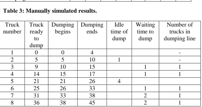
The manually simulated results are given in Table 3. For manual simulation, the random
numbers were dictated by the authors and this ensured that only one set of correct manual
solution was generated. Other related results are given below:
Average production rate =
45 60 8x
= 10.67 trucks/hour.
Idle time for dumping operation = 5 minutes. Average number of trucks waiting to dump =
38 7
= 0.184
Discussions
The objectives of the module, simulation, consist of (Ku, 2008):
1. describe the use of the Monte Carlo simulation technique;
2. recognise a situation which lends itself to the use of the Monte Carlo simulation
technique;
3. analyse a simulation problem to provide data for workplace design;
4. evaluate a queuing situation using simulation.
Now, it is the time to find out the how the software packages satisfy the objectives of the
module. Only Excel inMS Office 2007 is able to solve the Monte Carlo simulation with two or more variables and they are shown in Figures 1 and 2 respectively. Only this package can
satisfy the objectives 3 and 4 of the module; this matches the desired outcomes as students
can analyse a simulation problem to provide data for workplace design and evaluate a
queuing situation using simulation.
The Excel in MS Office 2007 programming required in simulation is more than that required in solving programming techniques of module 2 of the course. For simple simulation
problems, POM-QM for Windows 3 is good for beginners as there is straight forward input to the template but it provides only solutions to problems with one variable; in ENG 4004, it is
intended to have simulations with two interdependent variables to make them interesting and
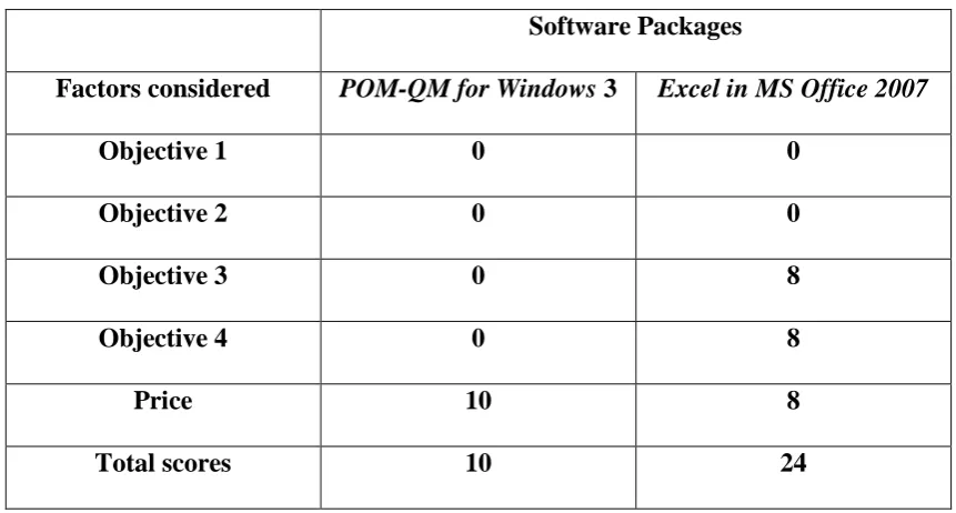
In order to decide which software package is better for the module, a pseudo quantity
evaluation method is employed, in which scores are allocated to each package when they
satisfy a particular objective of the topic. Score of 0 to 10 will be awarded to each package
for satisfying a particular objective, 10 being the highest and the package with highest total
scores is considered to be more suitable software for the module. Table 4 shows how scores
were allocated to the software packages. As the total scores of Excel in MS Office 2007 (24) is higher than that of POM-QM for Windows 3 (10), the former is therefore considered to be a more suitable package for the module.
Iglesias and Paniagua used of spreadsheets in an undergraduate course as a tool to solve
optimization problems with iteration cycles in the calculation of the variables involved and as
an introductory approach for the basic aspects of process simulators [9]. They were able to
appreciate the advantages of using a spreadsheet as work environment compared to other
environments; it turned out to be more powerful than GAMS or MathCAD. Another
important aspect is the possibility of incorporating new calculation procedures, in a simple
and transparent way, to the user form. The readiness of a powerful programming language,
such as VBA in the case of Excel, as well as the ease of recording, editing, and modifying
macros notably simplifies the task of preparing material to be used in the course. It is
advisable to use Solver (a macro function in Excel) to solve all iterations present in the
problem, still those that can be automatically treated by the spreadsheet [9].
The analysis made by Liberatore and Pollack-Johnson revealed strong differences in extent of
usage, type of usage, and software selection based on individually significant environmental
and intermediate factors. They also provided strong support for the hypotheses relating to
for the hypothesis relating to software use for planning only versus planning and control.
These results together validated the organizing framework. Adopters of project management
(PM) software were advised to consider the findings concerning industry practice as well as
their specific needs when selecting and deciding how to use PM software packages. Even
tough industry showed significant differences in the packages used, the two outstanding
packages were Microsoft Project and P3 (Primavera 3) [10]. The addition of the software
packages to the topics in the course will certainly improve the academic standing because its
contents are now at par with most of international textbooks. Students will also be able to
apply what they have learnt from the course to their workplace with ease as they will not
need to do complicated iterations or calculations. All are done by standard software packages.
The new form of assignments, in which students are required to solve problems using
software packages as well as manually, will be implemented in semester 2, 2009. . It can also
be argued that some authors are also working on something similar to the authors of this
paper. The difference between their work and this is that they use software packages to help
teaching engineering courses other than engineering management science but all are
enhancing their learning and teaching by using relevant software packages [11-16].
Conclusions
In the first paper in this series, the authors conclude that different software will be required to
solve different part of critical path network problems, i.e. cocktail software - POM-QM for Windows 3 and MS Project 2007 [4]. However, POM-QM for Windows 3 was to be able to solve most parts of a problem and was preferred. However, in the third paper in the same
numbers. It can still be argued that POM-QM for Windows 3 is good for demonstrating how simulation with one variable works to beginners.
Table 4 shows that POM-QM for Windows 3 is unable to solve problems of Objectives 1
through 4 while Excel in Microsoft Office 2007is able to solve problems of Objectives 3 and
4 but not those of Objectives 1 and 2. Their prices are equally friendly as Excel comes with
MS Office2007 and POM-QM for Windows 3 comes with the text book. Overall, Excel is
better and scored 24 as depicted in Table 5. This was also indicated by Iglesias and Paniagua
[9].
Other free spreadsheet packages such as OpenOffice, Calc, Gnumeric and MATLAB can be
argued to be able to perform what Excel in MS Office 2007 can perform in this study. Google Docs, a spreadsheet or similar online packages are likely to have the same functionality.
However, students may not be familiar with programming them as only Excel programming
is taught in one of their academic courses. But, it can be argued that engineering students can
learn them with ease.
References
[1] Salahuddin, A, Computer Aided Education in Civil Engineering, Proceedings of the 5th
International Conference on Computing in Civil and Building Engineering, 1993, pp.907-914.
[2] USQ Handbook 2008, General Information Section,
[3] Turban, E and Erikson, W, Selecting Operations Research Software for Classroom
Microcomputers, Computer and Operations Research, Vo. 12, No. 4, 1985, pp.383-390.
[4] Russell, R and Taylor, B, 2006, Operations Management: Quality and Competitiveness in
a Global Environment, 5th edition, Wiley and Sons Inc.
[5] Ku, H and R Fulcher, Using computer software packages to enhance the teaching in
Engineering Management Science: Part 1 – Critical path networks, Journal of Computer
Applications in Engineering Education, 2008 (accepted for publication).
[6] Keytack H, 1994, Computers and industrial engineering education: perspectives from the
University of Toledo, Computers and Industrial Engineering,v 27, n 1-4 , pp. 517-520.
[7] Heizer J and Render B, Operations Management, 9th edition, Pearson/Prentice Hall, 2008,
pp. 795 – 815.
[8] Ku, H, Engineering Management Science, USQ Studybook, 2009, pp. 2.3-2.11.
[9] Iglesias, O A and Paniagua, C N, Use of Spreadsheets in Optimization Problems
Involving Iterations, Journal of Computer Application in Engineering Education, Vol. 7,
1999, pp. 227–234.
[10] Matthew J. Liberatore and Bruce Pollack-Johnson, Factors Influencing the Usage and
Selection of Project Management Software, IEEE Transactions on Engineering Management,
[11] Jiang, Y and Wang, C, On teaching finite element method in plasticity with
Mathematica, Journal of Computer Applications in Engineering Education, 2008, Vol. 16,
No. 3, pp. 233-242.
[12] Günal, M and Özcan, A, Open channel design using Visual Basic, Journal of Computer
Applications in Engineering Education, 2008, Vol. 16, No. 2, pp. 127-136.
[13] Carolina Álvarez-Caldas, C, García, J, Abella, B, González, A, Educational software to
design shafts and analyse them by FEM, , Journal of Computer Applications in Engineering
Education, 2007, Vol. 15, No. 1, pp. 99-106.
[14] Sean, X and Liu, Ming Peng, The simulation of the simple batch distillation of
multiple-component mixtures via Rayleigh's equation, Journal of Computer Applications in
Engineering Education, 2007, Vol. 15, No. 2, pp. 198-204.
[15] Prasad, K and, Sahoo, N C, A simplified approach for computer-aided education of
network reconfiguration in radial distribution systems, Journal of Computer Applications in
Engineering Education, 2007, Vol. 15, No. 3, pp.260-276.
Figure 1: Distribution of processing times for Processes A and B.
Figure 2: Random numbers and processing times for Processes A and B
Table 2: Random numbers for dumping and weighing
Table 3: Manually simulated results.
Truck number Truck ready to dump Dumping begins Dumping ends Idle time of dump Waiting time to dump Number of trucks in dumping line
1 0 0 4 -
2 5 5 10 1 -
3 9 10 15 1 1
4 14 15 17 1 1
5 21 21 26 4
6 25 26 33 1 1
7 31 33 38 2 1
8 36 38 45 2 1
Cycle time (minutes)
Frequency of occurrence
Weighing Dumping
1 2 3 4 5 6 7 8 9 10 3 6 12 30 40 45 32 21 8 3 4 8 20 30 50 56 20 8 3 1
200 200
Table 4: Scores to the two software packages used
Software Packages
Factors considered POM-QM for Windows 3 Excel in MS Office 2007
Objective 1 0 0
Objective 2 0 0
Objective 3 0 8
Objective 4 0 8
Price 10 8