Using ground penetrating radar (GPR) with multiple pass scans to improve 3D positional reliability of subterranean features

University of Southern Queensland

Faculty of Engineering and Surveying

Using Ground Penetrating Radar (GPR) with Multiple

Pass Scans to Improve 3D Positional Reliability of

Subterranean Features

A dissertation submitted by

Mr Christopher John Arnison

In fulfilment of the requirements of

Courses ENG4111 and ENG4112 Research Project

towards the degree of

Bachelor of Spatial Science (Surveying)

ABSTRACT

The use of Ground Penetrating Radar (GPR) has increased enormously over the past 25 years. One application for GPR that has gained popularity is the detection and location of underground utilities and subterranean features in the first few metres below the ground surface.

GPR typically uses frequencies in the range 30MHz to 1GHz. Signals are transmitted into the ground and radiate out in all directions in most solid materials. A fraction of the signal is reflected back by planar, point or linear features. The receiving antenna in the GPR collects the reflected signals. Current practice is to establish an X Y grid and perform a series of scans along each axis. The scans are then compiled into a 3D model. One of the limiting factors with GPR is in the interpretation of the outputs.

The accuracy of the 3D model relies on the positional accuracy of the GPR scan paths, the number of scans, and the frequency used. This project examines the benefits of scanning at extra angles in addition to the traditional X and Y directions. Specifically X + 45º and Y + 45º scans are investigated.

A test site containing various objects has been prepared. The location of all the target objects has been surveyed, prior to burying the objects. The test site was scanned using a variety of scanning patterns. 3D models were produced from different combinations of the GPR scans. The derived position of the objects from the different 3D models is compared against the surveyed positions.

i

Certification

I certify that the ideas, designs and experimental work, results, analysis and conclusions set out in this dissertation are entirely my own effort, except where otherwise indicated and acknowledged.

I further certify that the work is original and has not been previously submitted for assessment in any other course or institution, except where specifically stated.

Christopher John Arnison Student Number: 0050037988

ii

Acknowledgements

I would like to thank the following people for their help and support during the course of this project.

Dr Xiaoye Liu my supervisor for this project, has helped me to develop an academic structure and style for my writing.

People at my workplace R.T.A. (Roads and Traffic and Authority) have provided much needed moral support and helped create time and space for me to focus on this project. Mr Glenn Jacobson helped enormously with the supervision of the construction and baseline survey of the test site. Glenn also helped with the GPR field work. The ‘gang’ of workers at St Marys Depot who constructed the test site for their patience. It is not often that they are asked to very carefully bury pipes that do nothing.

My work supervisor Mr Gordon Bell, who has allowed a flexible approach to my workload. This helped me to meet the commitments involved in this project.

Mr Ray Gilmour at the R.T.A. has helped as a day to day sounding board. Chats with Ray helped me to clarify my thoughts.

ENG4112 Using GPR.doc iii

TABLE OF CONTENTS

ABSTRACT

LIMITATIONS OF USE

CERTIFICATION...I

ACKNOWLEDGEMENTS...II

TABLE OF CONTENTS...III

LIST OF FIGURES...VI

LIST OF TABLES...VI

LIST OF EQUATIONS...VI

LIST OF APPENDICES...VII

LIST OF APPENDICES...VII

ABBREVIATIONS AND TERMINOLOGY...VIII

1

INTRODUCTION... 1

1.1 PROJECT BACKGROUND... 2

1.1.1 Current Techniques... 3

1.1.2 How GPR 3D Models Compliment Existing Methods... 4

1.2 THE PROBLEM... 5

1.3 PROJECT OBJECTIVES... 5

1.4 CONCLUSIONS:CHAPTER 1 ... 6

2

LITERATURE REVIEW... 7

2.1 HISTORY AND DEVELOPMENT... 7

2.1.1 What is GPR ... 7

2.1.2 Principals of GPR... 8

ENG4112 Using GPR.doc iv

2.1.4 Types of GPR in Use ...14

2.2 APPLICATIONS OF GPR...15

2.2.1 Subsurface Plume Detection...16

2.2.2 Pavement Layer Analysis ...16

2.2.3 Detection of Voids...16

2.2.4 Detection of Buried Utilities...16

2.2.5 Archaeological Investigation...16

2.2.6 Geological Feature Analysis ...17

2.2.7 Forensic science ...17

2.3 RELEVANT GPRRESEARCH...17

2.3.1 Research Using GPR in a Grid...17

2.3.2 Signal Processing ...19

2.3.3 Image Processing...19

2.3.4 GPR Simulation ...21

2.3.5 Analysis Methods ...21

2.3.6 Problems Encountered with GPR ...22

2.4 CONCLUSIONS:CHAPTER 2 ...22

3

METHOD ... 23

3.1 INTRODUCTION...23

3.2 EXPERIMENT DESIGN...23

3.2.1 Requirements for Test Site...24

3.2.2 Reference Coordinate System ...24

3.2.3 GPR Scanning Patterns...25

3.3 SUMMARY...26

4

RESULTS ... 27

4.1 SUMMARY OF PROCEDURE...27

4.2 SELECTED TEST SITE...27

4.3 FIELD EQUIPMENT...30

4.4 DETAILED DESCRIPTION OF FIELDWORK...31

4.4.1 Baseline Survey...31

4.4.2 GPR Scanning Procedure...32

4.4.3 Processing of GPR Raw Data...32

4.4.4 GPR 3D Model Method 1 – Hyperbola Fit...33

4.4.5 GPR 3D Model Method 2 –Peak Point ...36

ENG4112 Using GPR.doc v

5

ANALYSIS AND DISCUSSION... 39

5.1 INTRODUCTION...39

5.2 BASELINE SURVEY...39

5.3 SUMMARY OF GPRRESULTS...39

5.3.1 XY Scans at 0.3 Offset ...40

5.3.2 XY Scans at 0.6 Offset ...40

5.3.3 All 45º Scans Combined ...41

5.4 SOURCES OF ERROR...41

5.5 BENEFITS OF 45º SCANS...42

5.6 PROBLEMS ENCOUNTERED IN THIS PROJECT...42

5.7 BENEFITS DELIVERED BY THIS RESEARCH PROJECT...43

6

CONCLUSIONS ... 44

6.1 INTRODUCTION...44

6.2 CONCLUSIONS...44

6.3 FURTHER RESEARCH AND RECOMMENDATIONS...45

ENG4112 Using GPR.doc vi

List of Figures

FIGURE 2-1:HOW A TARGET IS SEEN BY GPR ... 8

FIGURE 2-2:BLOCK DIAGRAM OF GPR ...12

FIGURE 2-3:THREE TYPES OF GPR OUTPUT...13

FIGURE 2-4:HORIZONTAL RESOLUTION...18

FIGURE 2-5:IMAGE SHOWING BEFORE AND AFTER MIGRATION...20

FIGURE 3-1:PROPOSED SCANNING PATTERNS...25

FIGURE 4-1:LOCALITY MAP...28

FIGURE 4-2:TEST SITE DURING CONSTRUCTION...29

FIGURE 4-3:COMPLETED TEST PIT...30

FIGURE 4-4:IDSDUO GPR AS USED...31

FIGURE 4-5:AUTOMATIC HYPERBOLA DETECTION...34

FIGURE 4-6:HYPERBOLA DETECTION PROCEDURE...35

FIGURE 4-7:PEAK POINT METHOD, PEAK IS MARKED...36

FIGURE 4-8:3DTIME SLICE IMAGE...38

List of Tables

TABLE 2-2:THEORETICAL VERTICAL RESOLUTION...21

TABLE 5-1:XYSCANS AT 0.3OFFSET...40

TABLE 5-2:XYSCANS AT 0.6OFFSET...40

TABLE 5-3:ALL 45º SCANS AT 0.6OFFSET...41

List of Equations

ENG4112 Using GPR.doc vii

List of Appendices

APPENDIX A:PROJECT SPECIFICATION

APPENDIX B:RAW DATA TABLES AND GRAPHS

ENG4112 Using GPR.doc viii

Abbreviations and Terminology

The following abbreviations and terms have been used throughout the text AHD71 The level datum adopted throughout mainland

Australian

Brownfield site A site with existing infrastructure and often many constraints

Dielectric A property of a material where electrical effects are conveyed other by conduction

EM Electro Magnetic

EMF Electromotive force

EMI Electro magnetic induction

GPR Ground penetrating radar, any type of radar use to investigate solid structures or subsurface features Greenfield site A site with no existing infrastructure, totally clear

of human made buildings, or structures

MGA94 Map Grid of Australia 1994, the adopted standard grid datum for surveys in Australia

Permittivity The ratio of electric displacement to electric field strength in a dielectric medium

RADAR acronym of Radio Detection and Ranging, using electro magnetic signals to detect distance and sometimes direction to a target.

ENG4112 Using GPR.doc ix

Utility Any of the services that modern society uses such as electricity, gas, communications, water, sewer. Utilities are often buried underground in urban areas.

Chapter 1: Introduction

ENG4112 Using GPR.doc 1

1

Introduction

The first few metres beneath the Earth’s surface are the interface between the world that humans inhabit and the underlying structure of the planet. This interface area is rich in living organisms and geological structures. This area also contains objects created or deposited by plants, animals and humans. Investigating the location and structure of subsurface features helps society better understand the environment. From deciding where to safely build a bridge, to unravelling how ancient civilizations lived, investigating the subsurface area has almost limitless applications.

One tool that can be used to investigate the near subsurface zone is Ground Penetrating Radar (GPR). This form of radar provides a non invasive and non destructive method of investigation. With frequencies chosen to penetrate most solid objects, an image can be generated by analysis of the reflected signals. With origins in the 1960’s GPR has developed into a mature technology that can be used been used to help map and survey a variety of subsurface features.

GPR does not provide a direct image representation of hidden objects, as x-ray or computer aided tomography does. Instead differences are detected in the return signal, resulting in variations in a composite image. Many features have typical ‘signatures’ that can be picked out by a trained operator. An image can be analysed by correlating known subsurface features with areas of the GPR image. For some features varying the path of the GPR over the target will result in different images. Therefore individual GPR scans can be used to make decisions about the position and likely makeup of the subsurface environment.

Chapter 1: Introduction

ENG4112 Using GPR.doc 2

There are several scenarios where the extra investment in time and effort to produce accurate 3D position for underground structures is justified. These include investigation into underground utilities for planning purposes (feasibility and design options), and maintaining a safe work environment on construction projects. Other situations arise where there is a limited time window to access a site. In these cases a systematic data collection procedure can be developed to capture as much raw data as possible. Post-processing the data offsite is then an option that allows detailed analysis.

1.1

Project Background

The detection and location of underground utilities has become a significant cost for construction projects in areas with existing infrastructure. This is particularly true of urban environments where competition for space is fierce. In brown field sites, it is estimated that the cost of locating, planning around and relocating utilities can be 10% or more of the project budget. Research by the Federal Highway Administration (FHWA) in the USA has found a cost benefit of $4.62 for every dollar spent on up front investigation (Lew et al 2000).

In addition to the cost implications there are serious safety risks present to construction workers, plus the consequential costs and inconvenience in disruption of services for extended periods. A series of power cuts to the CBD of Sydney in March and April 2009 were linked to damage to underground power cables (Sydney Morning Herald 2009).

The ability to determine what is underground via non destructive techniques is a necessary tool in modern society. There are a number of methods that can be used to achieve non invasive detection. These include: x-ray, ultrasound, magnetic detection, cable tracing (an induced electrical signal), acoustic monitoring, and analysis of chemical deposits.

Chapter 1: Introduction

ENG4112 Using GPR.doc 3

underground features. This is done by using GPR to produce cross sections at various locations on a site. These results can be marked up on the site, and if required surveyed via traditional methods. This would always be done with reference to surface features such as access lids, and utility owner plans.

One major application of GPR is the detection of underground utilities such as water, sewer, gas, electricity, and communications. This application of GPR will provide the focus in this dissertation when relating theory to the real world. There are many alternate methods that can be used to detect the presence of these services. GPR has advantages in the following areas; detection of non-conducting materials (eg: PVC, nylon, fibre optic cables), detection of isolated utilities (eg: concrete encased) and detection of abandoned buried infrastructure.

1.1.1 Current Techniques

GPR can be used to interactively determine where a difference in the sub surface material exists. When combined with other methods such as alternate field methods (eg: cable tracing), site intelligence, utility owner plans, council and other plans, GPR can provide answers where other methods fail to get a result. This method requires a degree of decision making in the field. The immediate results from GPR provide an image that requires interpretation.

In some cases buried utilities exist in locations with limited access (eg: rail lines, major roads, freeways and motorways). In these cases closing the rail line or road off to public traffic is the only safe way to perform field work. Because of the disruption, the time window to perform the fieldwork is limited. In these situations it can make sense to gather information and build a 3D model that can be analysed a later time.

Chapter 1: Introduction

ENG4112 Using GPR.doc 4

Locating the utilities accurately via non destructive methods is a costly exercise. It is not always possible to excavate into road surfaces as the cost of restoration work can become very expensive. Delays during the construction phase that require redesign and or rework of a project will lead to significant cost blowouts to the original budget. Therefore location of existing utilities up front during the planning phase is preferred.

1.1.2 How GPR 3D Models Compliment Existing Methods

There are many techniques used to detect and locate buried objects. All methods have particular strengths and weaknesses. GPR 3D models provide additional benefits such as a systematic field method that records GPR scans and position. The raw data can be traced back to a location in subsequent analysis. This also provides a good quality record in any subsequent dispute that may arise from damage to underground assets. Often underground services are concrete encased to provide support and a layer of protection. Methods such as non-destructive digging (NDD) do not (for very good reasons) expose services in these situations. However when excavation takes place at a future date, how do workers know that an underground service is embedded in the concrete? GPR can produce images that penetrate concrete and allow verification of a service’s position.

Chapter 1: Introduction

ENG4112 Using GPR.doc 5

1.2

The Problem

The underlying problem is the difficult task of locating buried utilities. Using GPR to locate buried utilities provides a complementary tool to other established methods. The interactive use of GPR is a highly interpretive task. The images that GPR presents do not provide a direct image of the subsurface. The image is distorted, mainly due to the fact that the GPR signal transmitted into the ground cannot be focused in a controlled direction, and the ground material characteristics can be highly variable.

Some of the short comings of 3D models include the lack of detail when conditions are not favourable for GPR. This can happen when the material being scanned is of a high conductivity or the area is cluttered with many objects.

When building a 3D model using GPR the follow general approach is followed. The target area is defined and an orthogonal grid is laid out. GPR scans are performed along each axis of the grid. The position of each of the scans is carefully recorded so that the scans can be combined into the 3D model. The 3D model provides an image of the target area, and can help to show the relationship of subsurface structures.

The problem is in interpretation of the 3D model in areas that are not favourable to GPR. Areas of clutter where unwanted reflections interfere with the desired targets are very hard to interpret with GPR. This project seeks to examine if additional scans can improve these situations.

1.3

Project Objectives

Chapter 1: Introduction

ENG4112 Using GPR.doc 6

The areas to be examined are:

• Resolution of scans, what is the minimum scanning density required to achieve maximum resolution

• Collect and analyse test data aimed at giving the quantitative benefits when collecting XY scans at 90º plus extra scans at 45º.

• Develop guidelines that can be used to establish if a 3D model can be generated successfully given that not all situations allow easy generation of 3D models.

1.4

Conclusions: Chapter 1

Chapter 2: Literature Review

ENG4112 Using GPR.doc 7

2

Literature Review

In this chapter a summary of the literature relating to the background, history and development of GPR will be presented. Following this some of the applications GPR is used for is presented. Finally, research that directly relates to the topic of this dissertation is explored.

2.1

History and Development

2.1.1 What is GPR

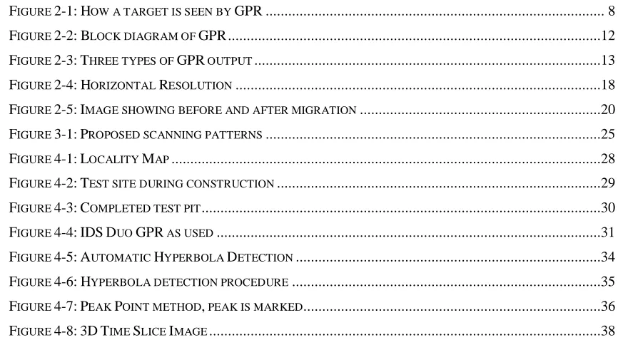
GPR is a class of radar that is designed to penetrate solid or visually opaque objects (including the region near the surface of the Earth). The specific category that GPR falls into is ultra wide band (UWB) radar operating in the frequency range 1MHz to 1GHz. Conventional, navigational, radar usually has a range of tens or hundreds of kilometres, whereas GPR has a range typically limited to tens of metres. GPR’s limited range is due to the attenuation characteristics of the material and varies with frequency (Manacorda 2006).

Chapter 2: Literature Review

ENG4112 Using GPR.doc 8

Figure 2-1: How a target is seen by GPR

(Manacorda 2006)

The resolution of GPR is of the order of centimetres, where conventional radar is of the order of metres to tens of metres. The main factor driving resolution is frequency (Manacorda 2006).

2.1.2 Principals of GPR

GPR comes with a complex set of variables and constraints. This section aims to explore the literature in terms of GPR as a system and the associated properties of the possible materials to be scanned with GPR.

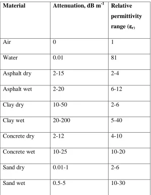
At the simple end of explanation is the concept of the propagation of electro magnetic (EM) waves and the way such waves respond to changes in the in the electro magnetic properties of the shallow subsurface. GPR generates a source signal, usually as a very short pulse, and transmits the signal into the ground. The GPR receiver detects changes in the electro magnetic properties by recording the return signals and displaying the intensity of the return signal relative to time.

Chapter 2: Literature Review

ENG4112 Using GPR.doc 9

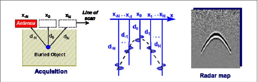
behaviour of EM wave propagation and material electro magnetic properties (Baker G, Jordan T, Pardy J 2007). Detailed exploration of these equations is beyond the scope of this paper. However the important concepts that relate to GPR are the material properties of relative permittivity ( r), magnetic permeability ( ), and conductivity ( ).

Typical values of relative permittivity ( r) for common materials measured at 100 MHz

are given in table 2-1.

Material Attenuation, dB m-1 Relative

permittivity range ( r)

Air 0 1

Water 0.01 81

Asphalt dry 2-15 2-4

Asphalt wet 2-20 6-12

Clay dry 10-50 2-6

Clay wet 20-200 5-40

Concrete dry 2-12 4-10

Concrete wet 10-25 10-20

Sand dry 0.01-1 2-6

Sand wet 0.5-5 10-30

Table 2-1: Attenuation and relative dielectric of materials at 100 MHz

Chapter 2: Literature Review

ENG4112 Using GPR.doc 10

GPR uses frequencies in the range 1 Mhz to 1 GHz. In this range a lot of the materials that make up the Earth’s surface can be thought of as a low pass filter (Daniels 2004, p131).

The main factors that influence the radar signal are:

• relative permittivity of the ground material - r

• magnetic permeability of the ground material -

• conductivity of the ground material -

• shape of point sources in the ground

• the interface between two types of material, including multiple interfaces

• depth to the target or interface

Radar relies on the time of flight to calculate a distance to a target reflection. Critical to the understanding of radar grams is the influence of dielectric properties on the speed of the radar signal. The attribute that influences speed of propagation is the relative dielectric constant ( r). Velocity of the GPR signal can be calculated using equation 2-1.

ε

ν

r

r

=

c

Equation 2-1: Velocity through medium

(Daniels 2004, p76)

Where r is the velocity, c is the speed of light in a vacuum, and r is the relative

Chapter 2: Literature Review

ENG4112 Using GPR.doc 11

number of different types of material, the dielectric constant varies. This results in a variety of velocities and resulting wavelengths.

The wavelength affects the maximum possible resolution of the images. In a vacuum or air the wavelength is virtually constant with frequency. However in other media, when the velocity varies the wavelength also decreases. As previously mentioned the properties of the medium will affect the velocity.

f

υ

λ

=

Equation 2-2: Wavelength

(Daniels 2004, p27)

Another important property that materials have is conductivity ( ). This together with

relative permittivity, effects the attenuation of the radar signal through the material (Daniels 2004, p21); also see table 2-1.

Grasmueck and Viggiano (2007) state, "For a heterogeneous subsurface, minimum grid spacing of GPR measurements has to be at least quarter wavelength or less in all directions". So for a radar frequency of 250 MHz in a material with a relative permittivity of 4 (dry sand), the wavelength is calculated to be 0.6m. Therefore the grid spacing for total coverage at this frequency would be 0.15m. Grasmueck and Viggiano go onto describe a technique for providing sub centre metre accuracy for GPR surveys using two or more rotating laser transmitters.

Chapter 2: Literature Review

ENG4112 Using GPR.doc 12

Figure 2-2: Block diagram of GPR

Chapter 2: Literature Review

ENG4112 Using GPR.doc 13

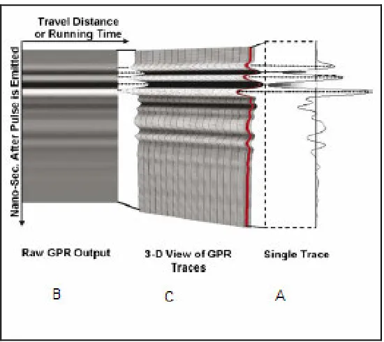
Figure 2-3: Three types of GPR output

(Lester and Bernold 2007)

2.1.3 History of GPR

Chapter 2: Literature Review

ENG4112 Using GPR.doc 14

Pulsed techniques were developed in the 1930's (Daniels 2004, p3). GPR has been used since the 1960's for geological applications (Reynolds 1997). These included determination of the polar ice cap depth. United States Army used GPR during the Vietnam War for seeking tunnels of the Viet Cong (Reynolds 1997). GPR was used on the Apollo 17 mission (Olhoeft 2002) and there are planned applications for GPR on future Mars missions (Pettinelli E et al 2007). In the Lunar experiments one advantage GPR had over seismic methods was the use of non contact transducers. This benefit meant the GPR could run with minimal human interaction, useful when time was short for these missions.

GPR has been used to detect sub surface features since the 1960's. Current applications of GPR are detailed in the section titled Applications of GPR. The use of GPR for engineering applications has accelerated since the mid 1970's.

2.1.4 Types of GPR in Use

The majority of GPR's are based on time domain impulse, or impulse radar (Daniels 2004, p35). This consists of transmission of a single sinusoidal pulse, and the subsequent detection and processing of the magnitude of the return signal. The advantage of this type of radar is the ease of manufacture. This type of GPR is the most common type commercially available, and is similar in concept to AM radio (Daniels 2004, p185).

Frequency modulated continuous wave (FMCW), are generally used at higher frequencies where it is hard to design an AM system (Daniels 2004, p211). In this type of GPR the frequency is changed over a known range, at a known time interval. The receiver compares the transmitted and received signal, and isolates phase changes due to the reflected signal from the medium. FMCW GPR have the following advantages: wider dynamic range, lower noise, and higher mean power.

Chapter 2: Literature Review

ENG4112 Using GPR.doc 15

and the dielectric of the ground being scanned. Non-contact can be operated at a distance above the ground and can be mounted on a vehicle such as a car or plane. In addition the configuration of the antennas can be varied as listed below:

Common source: this involves placing several receiving antennas that pick up signals from one source transmitting antenna. Common offset: the distance between the transmitter and receiving antennas is constant. This is the most common configuration. Common receiver: this involves placing several transmitting antennas that send signals to one receiving antenna (Daniels 2004, p34). In addition to these configurations specialised borehole GPR have been developed. Typically these have a common offset configuration, with the transmitting and receiving antennas travelling through the borehole.

The cheapest form of general purpose GPR is the hand pushed configuration, using a common offset configuration. These typically have a laptop computer to store and display radar grams.

2.2

Applications of GPR

There are many applications that use GPR. A small sample of the applications is listed below:

• detection and monitoring of polluting substances

• detection of road pavement layers and depths

• detection of voids under roads, near building foundations

• detection of buried utilities eg: gas, electricity, water, sewer and communications

• searching for and interpretation of archaeological remains

• mapping of geological features

• studying glaciological features including ice thickness, ice movement

Chapter 2: Literature Review

ENG4112 Using GPR.doc 16

The follow sub sections briefly describe some of the applications of GPR. Reynolds 1997, lists a total of 41 applications for GPR.

2.2.1 Subsurface Plume Detection

The spill of polluting substances heavier than water is one of the serious problems of environmental engineering. GPR can be used to track such spills over time, and help in the management of contaminated land (Daniels 2004).

2.2.2 Pavement Layer Analysis

A massive amount of research has been conducted on the use of GPR and pavement analysis. Due to the non contact advantage, and advances in the speed to pick up GPR scans, many solutions are emerging that allow a GPR to be towed behind a conventional vehicle. For some applications this is being performed at typical highway speeds. This application can be used for programmed maintenance, or quality testing. Highly accurate measurement of thin pavement layers is still being developed (Daniels 2004).

2.2.3 Detection of Voids

Voids by definition are air or another material within a structure. Because the dielectric properties of air differ from solid materials, GPR can be used to detect voids. This is useful for inspection and maintenance of structures.

2.2.4 Detection of Buried Utilities

This is the biggest commercial application for GPR (Euro GPR 2009). “The goal here is to map all the buried utilities and structures to enable rapid installation of new plant with the minimum of disruption” (Daniels 2004, p625). The two major limiting factors in the use of GPR for utility detection are: 1) attenuation of some soil types, and 2) density of utilities in certain cities.

2.2.5 Archaeological Investigation

Chapter 2: Literature Review

ENG4112 Using GPR.doc 17

destructive approach for consecrated ground. Secondly burials are often accompanied by important archaeological information (Reynolds 1997).

2.2.6 Geological Feature Analysis

GPR has been a valuable tool in the mapping of sedimentary sequences for geological mapping. This can be conducted on ground or in freshwater sites. Geological faults can be located when close to the surface (Reynolds 1997).

2.2.7 Forensic science

GPR has become a recognised method of forensic archaeology through some high profile cases. In the UK the high profile case of Frederick West came into the worlds headlines in 1994. After the discovery of West’s daughter’s remains, a wider search was organised. However due to the unsafe nature of the site, additional digging was ruled out. ERA Technology located suspicious sites for further investigation using GPR (Daniels 2004).

2.3

Relevant GPR Research

In this section, research that is relevant to this dissertation is presented.

2.3.1 Research Using GPR in a Grid

Using a standard grid search is a proven technique for many aaplications. However the required grid spacing is also a function of the size of target, orientation of target, and the contrast between target and surrounding material.

Approximate relationships between types of targets are: for the size and orientation of target a point scatter has an order of magnitude less received signal than a line reflector. A line reflector has an order of magnitude less received signal than a planar reflector (Daniels 2004, p18).

Chapter 2: Literature Review

ENG4112 Using GPR.doc 18

X Y grids were sampled one at 50cm spacing, the other at 25cm spacing (Y direction only). The results were compared against a single transect image. The conclusions stated there was minimal improvement between the 50cm and 25cm pattern for the increase in fieldwork effort. However the composite images for both X Y grids were able to resolve thin linear features not apparent from single transect orientation. The application that was the focus of this study was archaeological, the structures being building sized or partial remains of buildings. These findings have relevance to the focus of the research in this dissertation.

Another fundamental aspect of GPR that is highly relevant is, as the depth of the object reflecting the signal increases, the horizontal accuracy decreases, see figure 2-4.

Chapter 2: Literature Review

ENG4112 Using GPR.doc 19

2.3.2 Signal Processing

Signal processing is an internal function of most GPR units. However some knowledge of the types of signal processing can help to solve various problems. Because the GPR receiving antenna is measuring the amplitude of the signal with respect to time, the GPR must perform some form of signal processing to decode the signal and produce an image. Zero scan offset refers to a time offset that represents the surface of the ground. It is a time offset of the signal from the antenna to the first point of contact to the ground. This setting is usually constant with hand pushed GPR units, but may need adjustment if the antenna is raised for what ever reason.

DC drift refers to any offset in the A scan signal. If the mean value of the A scan is not zero noise will be apparent in the resulting B scan image. Noise reduction removes random noise from the A scans. Clutter reduction can be achieved by subtracting from each A scan an averaged value of a group of A scans or B scans over the area of interest (Daniels 2004).

2.3.3 Image Processing

The raw B scan or C scan from GPR does not represent the geometric shape of the target. Rather the raw scans display the reflection pattern. Migration is a process where the raw data is mapped to more accurately represent the shape of the target. This process has been developed and used by acoustic, seismic and geophysical engineering (Daniels 2004, p278).

Algorithms specifically developed for seismic applications rely on the antenna radiation patterns and the relative orientations of the antenna and target reflectors, these have been adapted for some uses in GPR (Streich 2007).

Chapter 2: Literature Review

ENG4112 Using GPR.doc 20

1. ReflexW™ by Sandmeier Scientifc Software 2007 2. GPR Slice™ by www.gpr-survey.com

Figure 2-5: Image showing before and after migration

(www.gpr-survey.com 2009)

Chapter 2: Literature Review

ENG4112 Using GPR.doc 21

2.3.3.1 Pattern Regognition

In their paper Liu et al 2008, propose a modified Hough Transform algorithm. They have included GPR hyperbola detection as one of their applications. The basic algorithm uses a weighting system to detect features. This is closely linked with research not related to GPR imaging, such as computer vision.

2.3.4 GPR Simulation

Simulation allows efficient investigation of specific areas of the problem. In their paper Wang and Oristaglio 2000, aim to simulate the behaviour of GPR in dispersive soils to detect pipes. Modelling with simulation tools allows a vast number of permutations to be trialled without the cost of conducting huge quantities of field work.

2.3.5 Analysis Methods

The simplest method to analyse the GPR data is to apply a line of best fit for each of the targets within the 3D model, however due to the distortions due to the variation in velocity, this approach is not always successful.

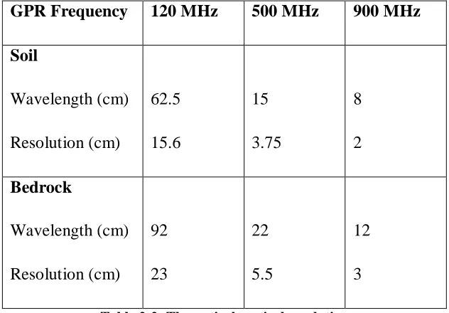
The following table 2-1, shows the theoretical vertical resolution at three separate frequencies.

GPR Frequency 120 MHz 500 MHz 900 MHz

Soil

Wavelength (cm) Resolution (cm)

62.5 15.6

15 3.75

8 2 Bedrock

Wavelength (cm) Resolution (cm)

92 23

22 5.5

12 3 Table 2-2: Theoretical vertical resolution

Chapter 2: Literature Review

ENG4112 Using GPR.doc 22

2.3.6 Problems Encountered with GPR

Examination of the literature has one common problem with respect of GPR. This is the interpretation of the radar grams. Because GPR does not provide a direct representation of the objects scanned, the images produced must be interpreted.

The other major problems are media where GPR does not work due to the dielectric properties of the materials being scanned, and clutter where many unwanted objects of varying materials serve to obscure the targets.

2.4

Conclusions: Chapter 2

It is very likely that many innovations will be combined by manufacturers into their offerings as GPR matures. The broad area of non destructive testing has many applications waiting for GPR to open up.

Chapter 3: Method

ENG4112 Using GPR.doc 23

3

Method

3.1

Introduction

This project aims to test different combinations of GPR scanning patterns and their effectiveness when producing 3D models of the target area. In summary the experiment will collect data for the same area using a variety of directional scans. Different combinations of these scans will then be analysed and compared to a baseline topographic survey using traditional survey methods. To help understand how different combinations of scans affect the 3D model, an understanding of all the variables that go into producing each dataset is critical. Some of the variables cannot be varied due to practical limitations on the available equipment, for example only one type of GPR is available with two fixed frequencies.

The fundamental issue being examined is the measured position of objects using GPR. To determine how well this measurement task is being performed a baseline survey of the target positions needs to be independently obtained. To be able to quantify any errors, the independent measurements need to have an equal or better level of accuracy. The simplest method to provide a good quality survey is to measure the position of the targets using a total station. This could be done on a live site with real utilities, either before they are covered for a new site, or investigated using non destructive digging on an established site. Alternately a test pit could be prepared. As the test pit is carefully filled, various objects can be placed and their position measured.

3.2

Experiment Design

Chapter 3: Method

ENG4112 Using GPR.doc 24

The variables to be considered are: the type of material that the scans are performed on; position and orientation of buried targets; surveyed position of targets to be used as a base comparison; surveyed position of GPR scans; GPR frequencies used; profile spacing interval (ie: density of scans); and lastly the

1. Type of material being scanned, dielectric properties (ie: sand, clay). 2. Position and orientation of buried targets

3. Surveyed position of GPR scans. 4. GPR frequency used.

5. Profile spacing interval (ie: density of scans)

6. Analysis of datasets, how will they be analysed? Statistical analysis methods? 7. Lastly, the factor that is being tested ie: the scanning pattern XY, XY+45,

XY+45+135

3.2.1 Requirements for Test Site

The test site should have a variety of fill materials, also the test site should have a variety of target materials to provide variation in the targets to detect. Both of these attributes help to simulate real world conditions. The test site should also have a smooth surface to allow trouble free use of the GPR equipment.

The RTA had already proposed to build a test pit to help with the testing of underground location equipment and enhancement of locating skills. The above requirements were added to the design of this test pit.

3.2.2 Reference Coordinate System

Chapter 3: Method

ENG4112 Using GPR.doc 25

3.2.3 GPR Scanning Patterns

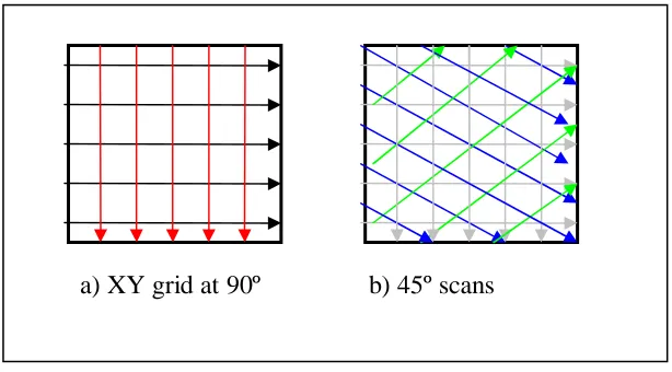
The pattern that the GPR scans are performed in is central to this project. Figure 3-1 shows the two basic scanning patterns. The XY pattern at 90º is the traditional pattern adopted for grid surveys. The 45º are scanned at the same time, but saved in a different GPR project.

Figure 3-1: Proposed scanning patterns

A grid will be marked at the required scanning interval for the XY scans. To maintain a common offset between scans a separate grid will need to be marked for the 45º scans. This offset can be calculated from the Pythagoras relationship for a right angled triangle.

To calculate the maximum density of the scans required to obtain maximum resolution, the relative permittivity needs to be determined for the GPR frequency. As a guide at 700 Mhz for a dielectric of 6, a wavelength of 0.175m is calculated (using equations 2-1 and 2-2). Therefore the grid required to gain the maximum information is 0.044m. For an area of 10m by 5m this would require 112 x 10m scans in the X direction, and 222 x 5m scans in the Y direction. The sum of all these XY scans is 2230m. The diagonal scans would add to this by a factor of more than 1.

Trial scans were performed to see if there was any noticeable difference between scans at the 0.045 interval. For a limited sample size conducted at random positions on the test

Chapter 3: Method

ENG4112 Using GPR.doc 26

site no difference was detected at this interval. To keep the fieldwork practical a sampling interval of 0.3m was chosen for the XY grid offset. The 45º scan offset was chosen at 0.6m which is a multiple of 0.3. It is intended to compare the XY data set de-sampled to 0.6 with the 45º data set. These scanning offsets were primarily chosen for simplicity and to keep the field work to a manageable level.

3.3

Summary

It is important that the GPR scans are performed at the same time. Moisture variation is the most common issue when attempting to combine scans from different dates. As highlighted in the literature review, water has a very high dielectric constant, so even a small variation in moisture levels can greatly affect the GPR results.

Chapter 4: Results

ENG4112 Using GPR.doc 27

4

Results

In this chapter summarised results of the fieldwork are presented. The full set of result data is presented in appendix B and appendix C.

4.1

Summary of Procedure

The underground baseline survey field work was conducted during August 2009 as the test site was being constructed. The surface baseline survey and GPR scanning work was performed on the 8th September 2009. The results from the fieldwork were collated into three datasets; the baseline survey, the 90º GPR scans, and the 45º GPR scans. The baseline survey is easily converted into XYZ coordinates by traditional survey reduction techniques. In this project the software MX V8 XM™ was used. This software performs two functions in this project. Firstly all total station radiations are reduced to MGA94 and AHD71 datum. Secondly, MX is used as a CAD package to prepare plans and cross sections. All survey control was referenced to three control stations at the site, details of the survey control network are given in appendix C.

The GPR data was collected using the IDS Duo Onboard Software. Separate IDS projects were setup for the 90º GPR scans, and the 45º GPR scans. These IDS projects were analysed using a stand alone package GPR Slice™. Tables, graphs and statistical summaries were prepared using MS Excel™.

4.2

Selected Test Site

Chapter 4: Results

ENG4112 Using GPR.doc 28

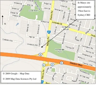
Figure 4-1: Locality Map

The locality map in figure 4-1 shows the approximate location of the test site. The site was built at the RTA St Marys Depot, on the outskirts of Sydney, Australia.

St Marys site

approximately 35km East to Sydney CBD

© 2009 Google – Map Data

Chapter 4: Results

ENG4112 Using GPR.doc 29

Figure 4-2: Test site during construction

Figure 4-2 shows the test pit during construction. The targets can be seen still partially exposed. The targets are surveyed before carefully burying them. Targets from left to right are: fibre optic cable (direct buried), 32mm nylon gas pipe, fibre optic cable (direct buried), 50mm electrical conduit PVC, 100mm electrical conduits PVC (3 pipes), metal pipe [WM01], 100mm stormwater PVC.

Chapter 4: Results

ENG4112 Using GPR.doc 30

Figure 4-3: Completed test pit

The completed test pit had a survey of the final ground surface. This survey captured the slope of the site, plus ground features such as pits, edge of concrete, edge of bitumen.

4.3

Field Equipment

The list of major equipment as used in the gathering of the field data is as follows: 1. IDS Duo GPR. A photo of the GPR can be seen in figure 4-3. The radar can be

pushed forward or pulled backwards. In this project the GPR was always pushed forward to provide consistency.

Chapter 4: Results

ENG4112 Using GPR.doc 31

Figure 4-4: IDS Duo GPR as used

4.4

Detailed Description of Fieldwork

4.4.1 Baseline Survey

The baseline survey was performed using a Leica Total Station and associated ranging pole, prisms etc. These survey points were reduced and plotted using the software MX V8 XM. This process is a standard surveying process used for many trigonometric surveys. Significant care was taken during this process as these readings formed the ground truth values for later comparison. Multiple check shots to the survey reference stations were made during this survey. However no redundant readings were taken of the measurements, therefore an error for this portion of the field work cannot be derived. A probable error of +/- 5mm has been adopted as this is considered a common

Laptop for storage and display

Signal

Processor

Antennas

Distance counter

on wheel Reference

Chapter 4: Results

ENG4112 Using GPR.doc 32

industry standard for this type of survey work. This takes into account manually holding the ranging pole, placing the ranging pole on the desired centreline of the feature to survey.

4.4.2 GPR Scanning Procedure

The GPR scanning grid was maximised to fit the site. This measured 11.4m by 6.0m at 0.3m spacing for the XY grid. To keep the 45º scans at the same offset, a grid spacing at 0.85m was marked out. When swung 45º this gives a spacing between scans of 0.6m. The end points of all grid lines were surveyed.

The GPR scans were all taken in the forward direction and recorded to the IDS project file. The GPR unit was aligned with the edge of the grid. In total 99 scans were recorded corresponding to the grid offsets as outlined about. A survey plan of the scans is available in appendix C.

The counter wheel on the GPR unit was checked against a tape measure. The results are as follows:

Tape: 14.995m GPR Wheel: 15.25m

This gives an error factor for the counter wheel of 1.7%

4.4.3 Processing of GPR Raw Data

Chapter 4: Results

ENG4112 Using GPR.doc 33

GPR radar-grams. These marked positions can then be joined together for linear targets thereby producing a 3D model in raw coordinates.

The common steps to import GPR data into GPR Slice™ are as follows: 1. Import raw GPR files

2. Define spatial relationship (ie: end points and length of each scan)

3. Adjust the gain of the raw GPR data files to maximise signals at greater depths 4. Define the zero scan that represents the ground surface (ie: zero offset for

vertical direction)

5. Optionally, additional filtering maybe applied to help highlight the desired features (eg: bandpass filtering)

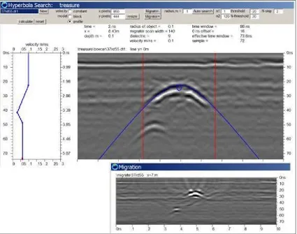
4.4.4 GPR 3D Model Method 1 – Hyperbola Fit

Chapter 4: Results

ENG4112 Using GPR.doc 34

Figure 4-5: Automatic Hyperbola Detection

Chapter 4: Results

ENG4112 Using GPR.doc 35

Figure 4-6: Hyperbola detection procedure

Figure 6 shows the process of adjusting the fit of the hyperbola. The step in figure 4-6a) shows the dielectric value set too high, in figure 4-6b) the dielectric value set too low, in figure 4-6c) the dielectric value is set to match the target. In figure 4-6d) the matched hyperbola has been marked and recorded (to a log file), this provides an offset value and depth for the peak of the target in metres. The end points of the scan can be used to derive the third coordinate required to define the point in 3D space.

The tables and graphs in appendix B from page B-2 to B14 are the formatted results for this hyperbola fit method.

a)

b)

c)

Chapter 4: Results

ENG4112 Using GPR.doc 36

4.4.5 GPR 3D Model Method 2 –Peak Point

The Peak Point method is a manual process of picking the peak of the hyperbola. The dielectric of the medium has been defined before this process of marking the peak is performed. The coordinates of the peak are stored in a log file and are easily retrieved for later analysis.

Figure 4-7: Peak Point method, peak is marked

Figure 4-7 shows one hyperbola that has been marked on the peak. This process is a manual process where the mouse cursor is finely adjusted onto the peak. A click of the mouse then marks the desired point. The horizontal scale is the distance as measured by the GPR counter wheel, while the vertical scale is the depth as calculated via time of flight. The vertical scale on the right is given in units of time, while the vertical scale on the left is distance calculated from the time and adopted dielectric value for the fill medium.

Chapter 4: Results

ENG4112 Using GPR.doc 37

4.4.6 GPR 3D Model Method 3 - Time Slice

One of the major features of GPR Slice™ is the ability to interpolate between several GPR scans and graphically analyse the GPR images in three dimensions. This was the intended process to use for analysis in this project. However due to high reflectance values not related to the desired targets (ie: clutter), this method did not produce consistent results that could be used. Therefore the manual hyperbola marking procedures were adopted.

In addition to the 5 common steps as defined in 4.4.2 Processing of Raw GPR Data, the following steps are applied to produce a 3D time slice model. The time slice approach aims to combine the vertical radar grams into a 3D model. The model is then sliced horizontally to provide a plan representation of the subject area.

1. The slice-resample step divides the radar grams into time intervals

2. The second step in the slice-resample assigns a weighting in the horizontal plane into the cells that represent an area at a given time depth

3. The gridding step performs interpolation horizontally between adjacent cells. Several options exist to control the mathematical weighting between adjacent cells

4. Gridding part 2, applies a filtering process eg: low pass or box car filter between these cells

5. A final construction step builds pixel maps and a 3D model.

Chapter 4: Results

ENG4112 Using GPR.doc 38

Figure 4-8: 3D Time Slice Image

Figure 4-8 shows an image prepared using GPR Slice™. The faint outline of the metal pipe (WM01) can be seen. There are many points of high reflectance in the top left corner of the image. The faint line of the pipe becomes lost in the points of high reflectance. This is due to the common problem of clutter where many unwanted targets of high reflectance are present in one area.

Chapter 5: Analysis and Discussion

ENG4112 Using GPR.doc 39

5

Analysis and Discussion

5.1

Introduction

The detailed calculations were made for one target in the test site only. This target was the metal pipe (WM01). This target was chosen as it had the most consistent signals in the GPR radar grams. If time allowed other targets could be examined using the same method, however as already mentioned considerable time was spent trying to produce a solution via time slice images.

The major finding was that the vertical position as derived was improved when using the 45º scans, while the horizontal position worsened. The results are provided in full in appendix B.

5.2

Baseline Survey

The baseline survey is a traditional total station 3D survey. Checks to the control stations were performed at regular intervals. As previously mentioned there is no independent verification of the total station radiations, so a nominal error of +/- 5mm is to be adopted. This is typical for close radiations from a total station in good conditions.

5.3

Summary of GPR Results

Chapter 5: Analysis and Discussion

ENG4112 Using GPR.doc 40

5.3.1 XY Scans at 0.3 Offset

Horizontal

Error Vertical Error Surv - Surv - Surv - Surv -

T Offset

Line BF

Z Offset

Line BF

WM01 XY GPR scans at 0.3 offset - hyperbola fit

Mean 0.042 0.040 -0.037 -0.037

Std

Error ± 0.027 0.004 0.031 0.034

Max absolute error 0.112 0.043 0.026 0.059

WM01 XY GPR scans at 0.3 offset - peak

point

Mean 0.024 0.020 -0.008 -0.014

Std

Error ± 0.033 0.005 0.040 0.034

Max absolute error 0.072 0.025 0.115 0.082

Table 5-1: XY Scans at 0.3 Offset

These scans have been done at the maximum scanning density at 0.3m between adjacent scans in both the X and Y directions. These results should provide the best results if the scan density is the main factor affecting accuracy.

5.3.2 XY Scans at 0.6 Offset

Horizontal

Error Vertical Error Surv - Surv - Surv - Surv -

T Offset

Line BF

Z Offset

Line BF

WM01 XY GPR scans at 0.6 offset - hyperbola fit

Mean 0.040 0.040 -0.035 -0.035

Std

Error ± 0.026 0.004 0.029 0.037

Max absolute error 0.089 0.043 0.026 0.059

WM01 XY GPR scans at 0.6 offset - peak

point

Mean 0.027 0.026 -0.006 -0.008

Std

Error ± 0.030 0.005 0.043 0.036

Max absolute error 0.062 0.029 0.115 0.083

Chapter 5: Analysis and Discussion

ENG4112 Using GPR.doc 41

The XY scans at 0.6m offset are a de-sampled set of the 0.3m set of XY grid. This set provides a direct comparison for the 45º scans.

5.3.3 All 45º Scans Combined

Horizontal

Error Vertical Error Surv - Surv - Surv - Surv -

T Offset

Line BF

Z Offset

Line BF

WM01 All 45º GPR scans at 0.6 offset - hyperbola fit

Mean 0.071 0.074 0.000 -0.001

Std

Error ± 0.072 0.036 0.027 0.018

Max absolute error 0.224 0.129 0.060 0.047

WM01 All 45º GPR scans at 0.6 offset - peak point

Mean 0.047 0.057 -0.011 -0.012

Std

Error ± 0.064 0.016 0.033 0.015

Max absolute error 0.203 0.080 0.043 0.032

Table 5-3: All 45º Scans at 0.6 Offset

The points to note about this set of data is difference for the horizontal and vertical standard error when compared to the XY scans at 0.6 and even the XY scans at 0.3. The horizontal standard error for the 45º scans is worse by about a factor of 2 (eg: 0.064 verses 0.030). However the vertical standard error for the 45º scans is better by about 30% (eg: 0.033 verses 0.043).

5.4

Sources of Error

The major sources of error are:

• the wheel counter error +1.7% for horizontal measurements

Chapter 5: Analysis and Discussion

ENG4112 Using GPR.doc 42

• vertical error for GPR targets dependent on zero scan setting, manually set. Also dependent on the manual hyperbola peak marking process.

• errors in total station radiations (typically +/- 5mm)

These sources of error are reflected in the summary statistics. Further work is required to quantify these sources of error further.

5.5

Benefits of 45º Scans

The main benefit of performing 45º scans is to increase the vertical accuracy. However this comes at a considerable processing overhead. The layout of a diagonal grid is more time consuming than a regular orthogonal grid.

Reasons for this improved result are not immediately clear. It could possibly be due to a higher number of GPR scans hitting the target given the scan takes a longer path over the target.

5.6

Problems Encountered in this Project

As previously mentioned the main problem encountered during this project was the lack of result achieved using the time slice image technique. Considerable effort was put into producing a result using this method. Some things to take away from this experience are:

• The need to look at methods to filter out clutter from the radar grams, this will enhance the results of time slice images

Chapter 5: Analysis and Discussion

ENG4112 Using GPR.doc 43

5.7

Benefits Delivered by this Research Project

Chapter 6: Conclusions

ENG4112 Using GPR.doc 44

6

Conclusions

6.1

Introduction

This project examined if using additional GPR scans at 45º improves the development and accuracy of a 3D model. Traditional 3D models from GPR scans use orthogonal scans (ie: X and Y scans at 90º). The 3D model was developed using two methods from the same raw data. The first method, which was largely unsuccessful, involved using a series of filtering and interpolation functions within the software GPR-Slice. The second method involved the manual selection of hyperbola (again using GPR-Slice) that matched linear targets in the test site. The coordinates of the selected hyperbola were calculated and manually joined to provide a series of coordinates representing the linear targets in the test pit.

6.2

Conclusions

In summary the 45º scans do not increase the horizontal accuracy of a 3D model produced by manually selecting hyperbolas. The standard error increases by a factor about two. However the vertical accuracy is improved by about 30% over orthogonal grids. This project has not investigated the reasons for the improvement in vertical accuracy for 45º scans.

Extra 90º scans improve accuracy in terms of helping to define the line of best fit. This is simply a function of increased number of samples statistically improving the result. Z offset error is proportional to the depth, because depth is calculated by applying a velocity correction factor, any error in this correction factor increases with depth, a larger time of flight (ie: when the reflected signal travels further).

Chapter 6: Conclusions

ENG4112 Using GPR.doc 45

6.3

Further Research and Recommendations

During the duration of this project several areas for further research were identified. The following detail a variety of research avenues that could be pursued.

The area of automatic hyperbola detection has been researched by others (Liu et al 2008), and partially implemented in the GPR Slice™ software. Enhancement of the user interface to better control automatic detection of hyperbola is recommended to increase productivity for this method. One method might be to train the hyperbola detector by initially manually selecting a sample. The automatic engine could then process the remaining selected scans, marking matches as it proceeded.

A checklist to determine if a GPR model is viable for a selected site would aid productivity. If a site can be assessed in a timely manner then GPR resources can be used at a higher efficiency. Issues such as clutter can prevent accurate location of targets. If these issues are discovered early in the field work process, unnecessary effort can be minimised.

REFERENCES

ENG4112 Using GPR.doc 46

REFERENCES

Baker G., Jordan T., Pardy J. 2007

An introduction to ground penetrating radar (GPR), The Geological Society of America Special Paper 432, 2007 Daniels 2004

Ground Penetrating Radar 2nd Edition, The Institution of Engineering and Technology, 2004

Euro GPR 2009

Guidelines for Utilities

www.eurogpr.org/guidelinesutilities.htm as cited: 16-Oct-2009

GPR Slice 2009

Image of Migrated Radargrams

www.gpr-survey.com as cited: 16-Oct-2009 Leckebusch 2003

Ground-Penetrating Radar: A Modern Three-dimensional Prospection Method, Archaeological Prospection, Volume 10 Issue 4, Pages 213 - 240

Lester & Bernold 2007

Innovative process to characterize buried utilities using Ground Penetrating Radar, Automation in Construction 2007, Volume 16, Issue 4, pages 546-555

Lew et al 2000

Lew, Anspach, Scott, Slack, Cost Savings on Highway Projects Utilizing Subsurface Utility Engineering, Purdue University Jan 2000

Liu et al 2008

REFERENCES

ENG4112 Using GPR.doc 47

Manacorda G 2006

IDS Radar Products For Utilities Mapping And Ground Classification, Trenchless Australasia Oct/Nov 2006 Metje, Rogers, & Chapman 2008

Seeing Through the Ground - Mapping the Underworld Project, The 12th International Conference of International Association for Computer Methods and Advances in Geomechanics, 1-6 October, 2008 Goa, India

Olhoeft GR. 2002

Applications and Frustrations in Using Ground Penetrating Radar, Aerospace and Electronic Systems Magazine – IEEE, Feb 2002, Volume: 17, Issue: 2

Pettinelli E et al 2007,

PETTINELLI Elena, BURGHIGNOLI Paolo, PISANI Anna Rita, TICCONI Francesca, GALLI Alessandro,

VANNARONI Giuliano, BELLA Francesco

Electromagnetic Propagation of GPR Signals in Martian Subsurface Scenarios Including Material Losses and Scattering, IEEE transactions on geoscience and remote sensing, 2007 vol 45 number 5

Pomfret J 2006

Ground-penetrating Radar Profile Spacing and Orientation for Subsurface Resolution of Linear Features, Archaeological Prospection, Volume 13 Issue 2, Pages 151 - 153

Radzevicius S 2008

Practical 3-D Migration and Visualization for Accurate Imaging of Complex Geometries with GPR, Journal of Environmental and Engineering Geophysics, June 2008 Reynolds J 1997

Reynolds John M., An Introduction to Applied and Environmental Physics, 1997 Wiley

Streich 2007

REFERENCES

ENG4112 Using GPR.doc 48

Surveying Regulations NSW 2006 Sydney Morning Herald 2009

Article: Blame for power cut in dispute, Sydney Morning Herald 30-Apr-2009

Wang T, Oristaglio M 2000

Appendices

A: Project Specification

B: Raw Data Tables and Graphs

CONTENTS APPENDIX B

Page

B-2 Summary Hyperbola Fit Method

B-3 WM01 XY GPR scans at 0.3 offset - hyperbola fit

B-5 WM01 XY GPR scans at 0.6 offset - hyperbola fit

B-7 WM01 Transverse 45º GPR scans at 0.6 offset - hyperbola fit

B-9 WM01 Longitudinal 45º GPR scans at 0.6 offset - hyperbola fit

B-11 WM01 All 45º GPR scans at 0.6 offset - hyperbola fit

B-13 WM01 All GPR scans combined - hyperbola fit

B-15 Summary Peak Point Method

B-16 WM01 XY GPR scans at 0.3 offset - peak point

B-18 WM01 XY GPR scans at 0.6 offset - peak point

B-20 WM01 Transverse 45º GPR scans at 0.6 offset - peak point

B-22 WM01 Longitudinal 45º GPR scans at 0.6 offset - peak point

B-24 WM01 All 45º GPR scans at 0.6 offset - peak point

B-26 WM01 All GPR scans combined - peak point

Summary of Hyperbola Fit Errors

S

u

rv

T

O

ff

s

e

t

S

u

rv

L

in

e

B

F

S

u

rv

Z

O

ff

s

e

t

S

u

rv

L

in

e

B

F

WM01 XY GPR scans at 0.3 offset - hyperbola fit

Mean 0.042 0.040 -0.037 -0.037

Std Error ± 0.027 0.004 0.031 0.034

Max absolute error 0.112 0.043 0.026 0.059

WM01 XY GPR scans at 0.6 offset - hyperbola fit

Mean 0.040 0.040 -0.035 -0.035

Std Error ± 0.026 0.004 0.029 0.037

Max absolute error 0.089 0.043 0.026 0.059

WM01 Transverse 45º GPR scans at 0.6 offset - hyperbola fit

Mean 0.076 0.081 -0.003 -0.005

Std Error ± 0.077 0.037 0.023 0.016

Max absolute error 0.224 0.133 0.032 0.037

WM01 Longitudinal 45º GPR scans at 0.6 offset - hyperbola fit

Mean 0.067 0.067 0.002 0.002

Std Error ± 0.071 0.036 0.031 0.022

Max absolute error 0.157 0.123 0.060 0.060

WM01 All 45º GPR scans at 0.6 offset - hyperbola fit

Mean 0.071 0.074 0.000 -0.001

Std Error ± 0.072 0.036 0.027 0.018

Max absolute error 0.224 0.129 0.060 0.047

WM01 All GPR scans combined - hyperbola fit

Mean 0.033 0.034 -0.009 -0.014

Std Error ± 0.048 0.008 0.037 0.027

Max absolute error 0.203 0.044 0.115 0.075

WM01 XY GPR scans at 0.3 offset - hyperbola fit L O ff s e t T O ff s e t L in e B e s t F it T S u rv T O ff s e t * S u rv T O ff s e t S u rv L in e B F Z O ff s e t L in e B e s t F it Z S u rv Z O ff s e t * S u rv Z O ff s e t S u rv L in e B F

1 0.0 1.92 1.90 1.94 0.02 0.042 0.75 0.72 0.78 0.03 0.06

2 0.3 1.88 1.89 1.93 0.05 0.041 0.74 0.72 0.76 0.02 0.04

3 0.6 1.88 1.89 1.93 0.05 0.042 0.74 0.71 0.74 0.00 0.03

4 0.9 1.87 1.88 1.92 0.05 0.042 0.76 0.71