University Of Southern Queensland Faculty of Engineering and Surveying
Carbon Offsetting through Soil Carbon Sequestration
for the Coal Mining Industry
An Application of a Soil Carbon Modelling
A dissertation submitted by
Mr Robert Handley
In fulfilment of the Requirements of
Bachelor of Environmental Engineering
ii
ABSTRACT
The purpose of this project is to produce a GIS model that collates information on land use, land management and soil type to develop a spatial model to assess the regional potential to sequester carbon. This model will be calibrated by assessing soil sampling data collected by NSW Office of Environment and Heritage and CarbonWatch data collected by HHM projects. Additionally best practice land use management in the region will be used to estimate soil carbon sequestration potential in the future and used to offset carbon emissions for an operational coal mine.
Managing the impacts of the mining industry on agricultural land and production as well as their operational carbon emissions are of increasing importance to the industry. Additionally with the advent of carbon tax, carbon trading schemes may be on the horizon and effective offsetting will become crucial to the industry.
Spatial information was compiled using existing mapping, Soil landscapes, topography, as well as district information on management practices and existing Soil Carbon levels. The compiled GIS model will be able to define a unique set of variables for any point within the study area, these variables will be analysed using the RothC carbon models to develop a spatial model of the regional soil carbon levels.
Assuming the best potential change in soil carbon as a result of best land management this paper found that approximately 322 ha of improved land management is required to offset every hectare disturbed by mining.
Further work is required to improve the accuracy of the required soil carbon model input variables.
iii
DISCLAIMER
University of Southern Queensland
Faculty of Engineering and Surveying
ENG4111 Research Project Part 1 &
ENG4112 Research Project Part 2
Limitations of Use
The Council of the University of Southern Queensland, its Faculty of Engineering and Surveying, and the staff of the University of Southern Queensland, do not accept any responsibility for the truth, accuracy or completeness of material contained within or associated with this dissertation.
Persons using all or any part of this material do so at their own risk, and not at the risk of the Council of the University of Southern Queensland, its Faculty of Engineering and Surveying or the staff of the University of Southern Queensland.
This dissertation reports an educational exercise and has no purpose or validity beyond this exercise. The sole purpose of the course pair entitled “Research Project” is to contribute to the overall education within the student's chosen degree program. This document, the associated hardware, software, drawings, and other material set out in the associated appendices should not be used for any other purpose: if they are so used, it is entirely at the risk of the user.
Professor Frank Bullen
Dean
v
ACKNOWLEDGEMENTS
This research was carried out under the principal supervision of Dr John McLean Bennett and Dr Lyndal Hugo (HHM Projects).
vi
TABLE OF CONTENTS
ABSTRACT ... II
DISCLAIMER ... III
CERTIFICATION ... IV
ACKNOWLEDGEMENTS ... V
LIST OF FIGURES ... VIII
LIST OF APPENDICES ... X
LIST OF APPENDICES ... X
ABBREVIATIONS ... XI
1.0 BACKGROUND AND OBJECTIVES ... 1
1.1INTRODUCTION ... 1
1.2PROJECT AIM ... 1
1.2.1 Objectives ... 1
1.2.2 Background ... 2
1.2.3 Timelines ... 3
2.0 LITERATURE REVIEW ... 4
2.1INTRODUCTION ... 4
2.1.1 Rationale ... 4
2.1.2 The Carbon Cycle ... 5
2.2IMPACTS OF LAND USE ON SOIL CARBON CYCLE ... 7
2.2.1 Agriculture ... 7
2.2.2 Mining ... 8
2.3EFFECT OF MANAGEMENT SYSTEMS ON SOIL CARBON SEQUESTRATION ... 9
2.3.1 Agricultural Management - Grazing ... 9
2.3.2 Agricultural Management - Cropping ... 10
2.3.3 Mining ... 11
2.4EFFECT SOIL TYPE ON CARBON SEQUESTRATION ... 11
2.5SOIL CARBON MODELLING ... 13
2.5.1 Land Use Management Factors ... 13
2.5.2 Soil Type Factors ... 13
2.5.3 Model Selection ... 14
3.0 METHODOLOGY ... 16
3.1STUDY AREA ... 16
3.1.1 Agriculture ... 16
3.1.2 Modelling ... 21
3.2ROTH CMODEL ... 21
3.2.1 Model Structure ... 21
3.2.2 Decomposition ... 22
3.2.3 Decomposed carbon partitioning ... 24
3.2.4 Radio Carbon Age and IOM ... 24
3.2.5 Required model inputs ... 25
3.3INPUT VARIABLES ... 26
3.3.1 Weather Variables ... 26
3.3.2 Soil Variables ... 26
3.3.3 Land use ... 34
3.4RUNNING THE MODEL ... 35
vii
3.4.2 Forward Modelling ... 39
3.5OFFSETTING ... 40
3.5.1 Carbon Emissions ... 40
3.5.2 Identify Potential Offset Areas ... 40
4.0 RESULTS ... 41
4.1CLAY PERCENTAGE ... 41
4.2LAND USE ... 42
4.3MEAN SOIL CARBON ... 45
4.4MAXIMUM SOIL CARBON ... 46
4.4.1 Analysis ... 49
4.5CHANGE IN CARBON ... 51
4.6CARBON EMISSIONS ... 52
5.0 DISCUSSION ... 55
5.1SOIL CARBON ... 55
5.2CHANGE IN CARBON ... 56
5.3LIMITATIONS AND FURTHER RESEARCH ... 57
5.3.1 Variables ... 57
5.3.2 Land Management ... 57
5.3.3 IOM ... 58
5.3.4 Clay Percentage... 58
5.3.5 Emissions ... 59
6.0 CONCLUSION ... 59
viii
LIST OF FIGURES
FIGURE 1 - THE CARBON CYCLE (RAVEN ET AL. 2004) ... 6
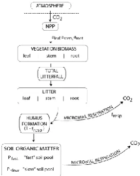
FIGURE 2 - PROCESS OF SOIL ORGANIC CARBON SEQUESTRATION. WHERE NET PRIMARY PRODUCTION (NPP) (FIELD & RAUPACH 2004) ... 6
FIGURE 3 - EFFECTS OF AGRICULTURE ON SOIL CARBON (FOLLETT 2001) ... 8
FIGURE 4 -LOCALITY PLAN ... 19
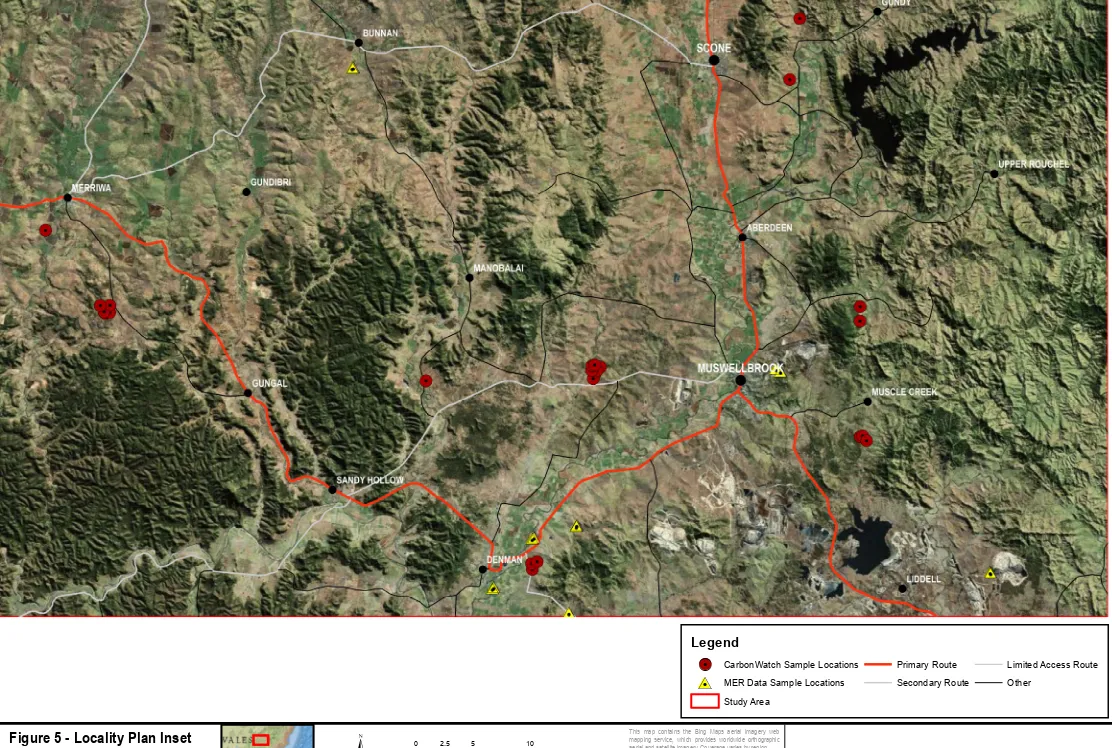
FIGURE 5 - INSET LOCALITY PLAN ... 20
FIGURE 6 - ROTHC CARBON MODEL STRUCTURE (JENKINSON & COLEMAN 1999) ... 22
FIGURE 7 - TRIANGLE TEXTURE DIAGRAM (MARSHALL 1947) ... 28
FIGURE 8 - ARCGIS LEFT IS DISSOLVE TOOL WHICH AGGREGATES FEATURES BASED ON SPECIFIED ATTRIBUTES AND TO THE RIGHT THE UNION TOOL WHICH COMPUTES A GEOMETRIC INTERSECTION OF THE INPUT FEATURES. ... 30
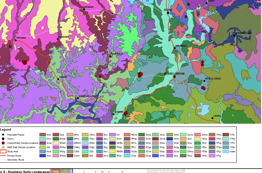
FIGURE 9 - SINGLETON SOIL LANDSCAPES ... 31
FIGURE 10 - SLOPES ... 32
FIGURE 11 - INSET OF STUDY AREA SHOWING GRID OF POINTS, THE MODEL WAS RUN AT EACH POINT . 35 FIGURE 12 - INPUTS FOR THE WEATHER FILE ADAPTED FROM (JENKINSON & COLEMAN 1999) ... 36
FIGURE 13 - THE INPUTS FOR THE LAND MANAGEMENT FILE ADAPTED FROM (JENKINSON & COLEMAN 1999) ... 36
FIGURE 14 - USER INTERFACE FOR THE INVERSE MODEL RUN ADAPTED FROM (JENKINSON & COLEMAN 1999) ... 38
FIGURE 15 - SCATTER PLOT FOR ESTIMATED PERCENTAGE CLAY VS. MEASURED CLAY. THE 45° LINE REPRESENTS A 1 TO 1 LINEAR RELATIONSHIP OF THE MEASURED DATA TO THE MODEL. .... 41
FIGURE 16 - PERCENTAGE CLAY ... 43
FIGURE 17 - ESTIMATED LAND USE ... 44
FIGURE 18 - SCATTER PLOT FOR ESTIMATED MEAN SOIL CARBON VS. MEASURED SOIL CARBON. THE 45° LINE REPRESENTS A 1 TO 1 LINEAR RELATIONSHIP OF THE MEASURED VALUES TO THE MODEL. ... 45
FIGURE 21 - SCATTER PLOT FOR ESTIMATED MAXIMUM SOIL CARBON VS. MEASURED SOIL CARBON. THE 45° LINE REPRESENTS A 1 TO 1 LINEAR RELATIONSHIP OF THE MEASURED VALUE TO THE MODEL... 46
FIGURE 19 - ESTIMATED MEAN SOIL CARBON ... 47
FIGURE 20 - ESTIMATED MAXIMUM SOIL CARBON ... 48
FIGURE 22 - TYPICAL SOIL CARBON CHANGE AS MODELLED BY ROTHC ... 51
FIGURE 23 - RATE OF SEQUESTRATION PATTERN FOR THE HIGHEST POTENTIAL SOIL CARBON CHANGE AS MODELLED BY ROTHC ... 52
ix
LIST OF TABLES
TABLE 1 - PROJECT TIMING PLAN ... 3
TABLE 2 - THE MAJOR INPUT VARIABLES FOR THE ROTHC MODEL... 25
TABLE 3 -TEXTURE CLASS AND (%) CLAY ... 29
TABLE 4 - MEASURED TOC AND CALCULATED IOM ... 34
TABLE 5 - REQUIRED SCENARIO FILE STRUCTURE ... 37
TABLE 6 - SUGGESTED VALUES FOR THE DPM/RPM VALUES (JENKINSON & COLEMAN 1999) ... 38
TABLE 7 - REGIONAL MINING CARBON EMISSIONS... 40
TABLE 8 - CORRELATION BETWEEN THE ESTIMATED SOIL CARBON AND MODEL VARIABLES ... 49
x
LIST OF APPENDICES
APPENDIX A - PROJECT SPECIFICATION ... 66
APPENDIX B - RISK ASSESSMENT ... 67
APPENDIX C - CALIBRATION RESULTS ... 76
APPENDIX D - SOIL LANDSCAPE ANALYSIS ... 78
xi
ABBREVIATIONS
AEMR Annual Environmental Management Report
ArcGIS A Geographic Information System Mapping Software
produce by ESRI
ASCII American Standard Code for Information Interchange
BIO Microbial Biomass
bMt Billion Metric Tonnes
BOM Bureau of Metrology
DPM Decomposable Plant Material
FAO Food and Agricultural Organisation
FYM Farm Yard Manure
HUM Humified Organic Matter
IOM Inert Organic Matter
NP National Park
NPP Net Primary Production
NSW New South Wales
OECD Organisation for Economic Cooperation and
Development
RPM Resistant Plant Material
SOC Soil Organic Carbon
TOC Total Soil Carbon
xii
1
1.0
BACKGROUND AND OBJECTIVES
1.1
Introduction
Managing the impacts of the mining industry on agricultural land and production as well as their operational carbon emissions are of increasing importance to the industry. Additionally with the advent of carbon tax, carbon trading schemes may be on the horizon and effective offsetting will become crucial to the industry.
The impacts of the mining industry of agricultural lands have also recently been the subject of many news headlines. Unfortunately the headlines often report the negatives of the industry. This study intends to promote the idea that industry may subsidise improved land management in return for the potential offsets, this idea could result in healthier soils and better farm management, higher production whilst offsetting some or all of the emissions of the mining industry.
This study focused on the modelling of the soil carbon with the study area, to reduce the scope of the above notion.
1.2
Project Aim
The purpose of this project is to produce a GIS model that collates information on land use, land management and soil type in order to develop a spatial model to assess the regional potential to sequester carbon. Additionally best practice management in the region will be used to estimate soil carbon sequestration potential and used to offset carbon emissions for an operational coal mine. This model will be calibrated by assessing soil sampling data collected by the Office of Environment and Heritage and HHM projects. The model will produced using arcGIS software.
1.2.1Objectives
1. Investigate, through the development of a spatial model and literature review, the potential increase in soil carbon achievable if best land management practices were employed throughout the Study area.
Identify dominant land uses and management practices within study area;
Outline best management practices for a particular land use;
2
2. Investigate the operational carbon emissions for a typical coal mine in the Hunter region.
Review Annual Environmental Management Reports (AEMR) for a typical mining operation, and determine average CO2 production.
3. Use the GIS model to estimate the offset potential of best management practices to sequester carbon emissions from an operational coal mine.
Identify areas of land required
Determine best areas for sequestering carbon
1.2.2Background
The soil carbon system is highly dynamic and involves numerous interactions between different systems. This study aims to develop a spatial model that has the ability to investigate the soil carbon sequestration potential in a regional context, and be able to manipulate land use to investigate the change to this potential. In order to determine this potential a number of study areas needed to be investigated throughout the literature review process. The literature review has been conducted and forms chapter 2 of this paper. The review focused on a number of study areas including:
Land use - Regionally dominated by Grazing, Cropping and Mining
Land Use Effects and Land Use Management Effects on Soil Carbon Sequestration
Soil Type effects on Soil Carbon Sequestration
Soil Carbon Models
Spatial Modelling Using Soil Carbon Models
Individually these topics are reasonably well understood and have been extensively studied. Models are typically a simplified version of reality and Soil Carbon models are no different. However as the dynamics of the reality that they are attempting to model are complex, soil carbon models are also complex. As a result, these models require a large amount of input data to achieve the best results. During a review of the required information it was found that a large amount of the required data for the carbon model will have to be assumed or obtained indirectly and this will likely affect the accuracy of the model.
3 Brazil with approximately the same latitude as the Hunter Valley and this study is proposing a similar methodology.
1.2.3Timelines
The main tasks to be undertaken by this study have been outlined below;
Literature Review
Project Appreciation Report
Producing an ArcGIS Model
Development of the Methodology
Field Work Collection of addition data as required
Results and Discussion
Project Seminars
Conclusions
Draft Dissertation
[image:15.595.123.531.471.732.2] Project Performance
Table 1 - Project Timing Plan
Task Duration Commencing Completion
Literature Review 8 weeks 25/03/12 23/05/12
Project Appreciation 1 weeks 16/05/12 23/05/12
Modelling 8- 10 weeks 23/05/12 18/07/12
Calibration of the model 8-10 days 22/04/12 08/06/12
Field work / Lab analysis of additionally
collected samples. 4-6week 08/06/12 20/07/12
Methodology write up 1 week 11/07/12 18/07/12
Results and discussion 4 weeks 18/07/12 15/08/12
Conclusions 2 weeks 15/08/12 29/08/12
Project Seminars 2 weeks 26/08/12 09/09/12
Draft Dissertation 4 weeks 29/08/12 26/09/12
Final/ Project performance 4 weeks 26/08/12 23/09/12
4
2.0
LITERATURE REVIEW
2.1
Introduction
2.1.1Rationale
The OECD places the world's 2006, 2010 population at 6.58 and 6.89 billion respectively and estimates that by 2050 this will reach 9.30 billion (OECD 2012). The current situation shows that many people are experiencing poverty and food shortages. In fact the FAO estimates that during the period between 2006-2008 there was an estimated 850 million people or 13% of the World's population suffering from undernourishment and malnutrition (FAO 2011). The problem lies with inequalities in the geographic distribution of food between developed and developing countries (Aplin et al. 1999). This trend highlights that there is a need to increase the world's food supply and to do this arable land is required. Therefore placing an increased value on the world's available arable land, thus protecting the quality of this resource should be of high priority.
Food production must be addressed if population growth is to continue as predicted. Whilst a substantial increase in food production is required to provide nourishment for the growing population this increase must also occur in a sustainable manner. Modern agricultural systems have evolved to become a high yielding, highly specialised, artificial ecosystem, requiring a high level technology, machinery, chemicals and genetics. The modern system has typically replaced complex "polyculture" with vast "monoculture" systems and substituted soil fertility with chemical fertilizers, animal and human labour with machines and fossil fuels and pest and weed control with chemical herbicides and pesticides (Aplin et al. 1999) and has enabled modern society to cultivate areas that are geologically and climatically very different to a crops natural environment. These systems have managed to achieve a production rate far above what is naturally capable, often be overexploiting the natural capacity of the land.
The over exploitation of the land has led to depletion of the lands ability for production. This term has been coined land degradation and includes impacts such as soil erosion, loss of fertility, soil structural change, salinisation, soil pollution and desertification (Aplin et al. 1999; Singer & Munns 2006). It is import that future agricultural process practice conservation and protection techniques to minimise the above effects on the land, as soil genesis is a very slow process and soil is currently the most critical strata in which agriculture and food is produced.
5 According to Charman and Murphy (2006) the main objectives of the sustainable framing are to maximise returns while maintaining the quality of soil, land and water while maintaining or improving ecosystems that are affected by agriculture. The major obstacles facing sustainable agriculture in Australia are land degradation, water use, chemicals use, vegetation destruction, biodiversity decline, pest and disease, feral animals (Aplin et al. 1999; Charman & Murphy 2006; FAO 2011; Hartemink & Hartemink 2003). Land degradation with particular focus on the soil includes the issues of soil erosion, loss of fertility, soil structural change, and salinisation (Aplin et al. 1999). These issues are particularly important as they can be directly related to management practices such as; excessive cultivation, bare soil and fallowing practices, overgrazing and lack of ground cover, traffic on wet soil, poor identification of land capability, clearing deep rooted natives and the use of acidifying pastures and fertilisers (Charman & Murphy 2006). It is therefore imperative that management practices are tailored to minimise the effect agricultural practices have on the surrounding environment and maximise the potential to produce food for future generations by maintaining the quality of productive lands.
There are a wide variety of agricultural systems that may be applied to an area depending on what cultivation method, weed control technique, crop selection, stocking rate and past land use has occurred. In addition, environmental factors such as weather, climate, landform, and the soils physical and chemical properties also influence the agricultural system applied. However regardless of the agricultural system applied, most of agricultural systems contribute to land degradation in some form. In a study completed by (Brejda et al. 2000), it was found the that soil carbon is the single most important factor influencing soil quality and health and many studies have also been completed linking soil carbon to reduced degradation and improved land productivity, additionally increasing carbon levels within the soil may even have the potential to offset or some of the effects of global climate change. For this reason soil carbon is being investigated in this study.
2.1.2The Carbon Cycle
6
Figure 1 - The carbon cycle (Raven et al. 2004)
The oceans contain an estimated carbon pool of 38,000 bMt of carbon which is stored as dissolved CO2. The atmospheric pool is approximately 780 bMt of carbon, in the form of gaseous CO2. An enormous proportion of carbon is stored in dead plants and animals as well as discarded shells, leaves and faeces. These products settle into the soil or oceans where they are decomposed. Decomposition processes release of CO2 into the atmosphere and ocean pools. The largest carbon pool (~18,000,000 bMt) exists as carbon in an inorganic form such as calcium carbonate the turnover of this pool is slow and release of CO2 is as a result of geological uplift and weathering. Another large source of carbon (~10000bMt) has been deposited in the form of coal and oil; these sources would also normally sequester carbon on a long term however human activity and the industrial revolution has resulted in the rapid consumption and re-release of these sources (Raven et al. 2004; Singer & Munns 2006).
Soil Organic Carbon (SOC) is another large pool of carbon (~1550bMt) (Follett 2001), SOC has accumulated as a result of partially decomposed material forming semi-stable carbon mineral complexes within the soil profile. Figure 2 shows a highly simplified process of soil carbon accumulation.
7 The time frame associated with soil carbon turnover ranges from less than 5 years to hundreds of years (Lal 1997). The rate of transition between each stage and the turnover in the soil is dependent on a variety of factors including soil type, climate, land use and land management.
Plant residue is the primary source of carbon input into a soil, specifically the amount of plant material and type of plant material returned to the soil affects soil carbon. Carbon forms such as cellulose, hemi-cellulose, and lignin's are broken down and incorporated into the soil at different rates. Cellulose and hemi-cellulous are broken down much more readily than lignin's, which are oxidised slowly and enriched with nitrogen to form a highly complex matter know as humus (Charman & Murphy 2006).
Climate, namely rainfall and temperature, affects the accumulation of soil organic carbon. Favourable climatic conditions aid the production of biomass. However, favourable climatic conditions also provide the environment for the existence of soil microbes, which increases the rate of SOC consumption. Generally in Australia our high temperatures and low rainfalls are not conducive to the accumulation of SOC when compared with the rest of the world (Carter et al. 1993; Charman & Murphy 2006). Modern agricultural practices often result in a major change to the local eco-system and climate. The clearing and replacement of natural eco-systems with vast monoculture systems changes the amount and type of plant material available as a source of carbon, while irrigation practices influence the local climatic conditions. Plant material generated from agricultural is traditionally removed to assist in the farming process and as a result this material is also removed as a source of soil carbon input. Practices such as irrigation and tillage affect the soil environment often providing favourable conditions for soil microbes that breakdown soil carbon, further reducing the soil carbon input.
2.2
Impacts of Land Use on Soil Carbon Cycle
2.2.1Agriculture
8
Figure 3 - Effects of Agriculture on soil Carbon (Follett 2001)
Brejda et al. (2000), found that soil carbon was an important indicator of soil quality. Soils carbon levels declined respectively with the following land uses; natural rangeland, conservational cropping and grazing practices and lastly conventional cropping (Brejda et al. 2000). This finding was expected due to the aggravation of the soil through tillage practices of the cropped land. It has been demonstrated that changes in land use management that focus on increasing plant productivity and decreasing soil disturbance, can result in the re-sequestration of some, if not all, of the lost carbon (Follett 2001).
2.2.2Mining
The process of open cut coal mining requires the stripping and stockpiling of soils and the removal of overburden to gain access to the coal resource. The landscape and soils are dramatically disturbed during this process and often result in soil degradation. The process of soil stripping and stockpiling can dramatically change the soil profile effecting the physical, chemical and biological soils properties and processes (Ussiri et al. 2006).
The rehabilitation of mined areas involves the placement and shaping of overburden and capping with the stockpiled soils to return the mined landscape to that of similar land suitability to the landscape that existed prior to mining. This process usually involves spreading, shaping and grading overburden applying topsoil, ripping and establishing vegetation. These processes have the objectives of minimising soil erosion, improving fertility and increasing soil biomass and productivity (Ussiri et al. 2006). The process of soil stripping and stockpiling results in high bulk densities, diminished soil structure, oxidation of soil organic matter, declined fertility and reduced soil fauna activity. As a result the success of the rehabilitation of mine soils is usually limited by these effects (Ussiri et al. 2006).
9
2.3
Effect of Management Systems on Soil Carbon Sequestration
2.3.1Agricultural Management - Grazing
Grazing can be summarised into continuous grazing with set or varying stocking rates, or rotational grazing with periodic paddock resting. These practices can occur on native or improved pastures. Traditionally grazing was continuous with high set stocking densities and since the 1950's industry has pushed towards improved pastures with high fertiliser inputs, unfortunately these pastures were usually sown exotic annuals from cool climates (Kemp & Dowling 2000). As a result, the majority of native grasslands and woodlands have been cleared often decreasing biodiversity. The changed land use has had considerable effects on soil structure and nutrient cycling (Dorrough et al. 2004; Yates et al. 2000).
Traditional grazing is attributed to a decline in biodiversity, soil ecosystem function, soil regulatory processes and soil structure, increased soil erosion, an increase in pest and weeds, and general land degradation (Cattle & Southorn 2010; Dorrough et al. 2004; Kemp & Dowling 2000; White et al. 2003; Yates et al. 2000). High stocking density results in overgrazing and leads to a reduction in cover and perennials, the decreased cover promoting an invasions of weedy exotic pastures resulting in a further declining biodiversity (Kemp & Dowling 2000). While the decrease perennial pastures result in the reduction of root mass when replaced with exotic annuals (Chan et al. 2010). Closed hoofed animals, through uneven foot pressures, affect the soil structure by changing the soils micro-topography, compaction, infiltration and erosion (Yates et al. 2000). Compaction and reduced infiltration can degrade the soil environment and reduce the potential to sequester carbon. Grazing reduces litter deposition, affecting habitat of soil cryptograms and reduces the amount of organic material available for carbon input (Cattle & Southorn 2010; Dorrough et al. 2004; Kemp & Dowling 2000; Yates et al. 2000). Yates et al. (2000) attributed the decline in ecosystem function and regulatory processes to a decline in soil nutrient cycling, due largely to a decline in the soil fauna activity and the transporting of nutrients within the soil profile.
Grazing at lower stocking densities results in preferential grazing of the most palatable species removing them from the area, this also results in bare patches promoting weed growth and generally degraded paddocks (Kemp & Dowling 2000). Understocked paddocks also often result in the transport of nutrients to stock camps (Dorrough et al. 2004). While high density grazing results in better pasture utilisation and reduces selective grazing, when practiced long term it results in the above mentioned degradation (Dorrough et al. 2004; Kemp & Dowling 2000; White et al. 2003).
10
managed high intensity, short duration grazing also maintained stable soil structure (Cattle & Southorn 2010).
Therefore it was found that rotational, time control and cell grazing, techniques that use high stocking densities, short grazing periods, and the tactical resting of land were the favoured management practices by the majority of the authors reviewed.
2.3.2Agricultural Management - Cropping
Current dry land cropping practices can be broadly summarised into conventional tillage, conservational tillage and zero tillage. These practices may occur concurrently with the removal or retention of stubble material. Conservational and zero tillage cropping have been developed with the aim of reducing soil disturbance, to slow the oxidation of soil organic matter and reduce loss of soil moisture. Stubble retention provides protection of the soil surface and increases the organic matter available for input while fallowing removes plant material and prevents soil carbon replacement (Charman & Murphy 2006). Conservational tillage through reduced soil disturbance, increased aggregation and improved soil structure leads to relatively high SOC content when compared to conventional tillage(Lal 1997).
Conventional tillage usually results in soil turnover which is detrimental to SOC (Lal 1997). Ploughing destroys soil aggregates exposing the previously unavailable SOC to soil microbes. Additionally, the aeration of the soil results in favourable conditions for soil microbes, which further accelerates the rate of soil organic matter breakdown through microbial respiration (Charman & Murphy 2006; Heenan et al. 2004; Lal 1997; Rimal & Lal 2009).
Conservational tillage and other management practices that improve levels of cover, fertility and focus on increasing plant residue contribute to a greater input of roots, plant biomass and other organic substances these increased SOC (Follett 2001; Rimal & Lal 2009). This is in line with Chan (2001) observation that the Total Organic Carbon (TOC) for continuously cropped, stubble retention soils was 20% higher than wheat-fallow soils. When this affect is combined with direct drilling, TOC levels were shown to be even higher (Chan 2001). Heenan et al. (2004) showed that a legume and wheat rotation maintained higher SOC than a wheat monoculture, retaining stubble in this rotation significantly reduced the mean rate of loss of SOC and the loss of SOC was significantly higher for conventional cultivation when compared to direct drilling management. This study also found the greatest rate of loss of SOC was measured under annual wheat cropping where the soil was conventionally cultivated and stubble burnt and concluded that the combination of direct drilling, stubble retention and a sub-clover phase resulted in the highest SOC. A majority of reviewed studies generally agreed with this conclusion. Dalal et al. (2011) added that SOC could be further improved through the addition of nitrogen fertiliser.
11 of changing from conventional to zero-till practices, with the best rates being achieved within 5–10 years. However Chivenge et al. (2007) reviewed other authors that estimated the same change in management could result in an average as low as 325+/-113 kg C ha-1 yr-1. Additionally the carbon turnover rate was estimated to be 1.5 times slower in zero-till compared with conventional systems (Chivenge et al. 2007).
A well-managed soil under conservation farming can maintain and gradually improve soil carbon, however the rate of increase is expected to be slow (Carter et al. 1993; Charman & Murphy 2006). This fits with the observations in Canada that show the change in SOC due conservation management practices are slow and that these changes may take approximately 25-50 years to approach a new equilibrium (Follett 2001). This affect is expected to be amplified due to Australia climatic conditions resulting in even longer to reach a soil carbon equilibrium (Carter et al. 1993).
In summary most cultivation practices result in a decline in soil carbon and this is attributed to the consumption of soil organic carbon through the process of microbial respiration. The majority of studies concluded that the best management of soil carbon was achieved through minimising disturbance to the soil structure, maintaining stubble and the balancing of nitrogen. These practices have the potential to reduce or even reverse soil carbon loss, particularly in favourable climatic conditions.
2.3.3Mining
As stated above mining has a dramatic effect on a soil and landscape. The overturning and disruption of the soil profile and the removal of vegetation are the main factors that influence a decline of soil carbon levels in post mined soils. Therefore the management of such soils will have the potential to reduce the impacts of these factors and influence soil carbon levels. The best practice guidelines for the handling of stripped soils focuses on soil moisture levels to help minimise compaction of the soil, the minimised handling of the mined soils to reduce the destruction of aggregates, the length of time the soil is stockpiled to reduce the decomposition of native seed and organic matter and the order of removal and reapplication in an attempt to minimise the effect on soil horizon blending (Landcom 2004). Once re-applied, vegetation and post land use activities are critical in restoring the quality and carbon content of the rehabilitated soils as vegetation results increased biomass productivity and root development which enhance the SOC levels (Ussiri et al. 2006).
While post reclamation land use and management are important, as shown above different cropping and grazing techniques have the potential to influence the carbon in soils. Best practice land use management should be used on rehabilitated mine soils to restore SOC as quickly as possible.
2.4
Effect Soil Type on Carbon Sequestration
12
classification. Whilst few studies investigate soil type effects, a number of studies outline the effects soil properties have on soil carbon accumulation. The soil properties that have the greatest effects on soil carbon are soil mineralogy and particle size distribution or soil texture (Chilcott, C. R. et al. 2007; Chivenge et al. 2007; Krull et al. 2001; Lal 1997). Other properties such as water holding capacity, pH and porosity act as modifiers to the rate of carbon sequestration (Krull et al. 2001). The amount of carbon within a soil is dependant mainly on two factors; these are soil carbon turnover time and physical protection provided by the soil (Lal 1997). Turnover time is dependent on the composition and size of the organic matter. Fresh biomass has a quick turnover time as it is rapidly decomposed by microbes. Humus and light fraction carbon have a moderate turnover time, less than 20 years, and exist between soil aggregates. While passive carbon may form complexes with clay minerals within the soil thus resulting in long turnover times of greater than 100 years (Lal 1997).
Soil mineralogy is a product of soil formation processes and source minerals. The accumulation of carbon in soils with high cation-exchange capacity, particularly with Ca2+, or soils with either or both amorphous iron or aluminium is well documented. Calcium containing soils often results in the stabilisation of SOC, through the precipitation of Ca2+ which results in a protective carbonate coating of freshly decomposed biomass. In more decomposed biomass often the positively charged Ca2+ ion acts as a linking molecule between negatively charged organic functional groups with either, other organic functional groups or clay surfaces (Krull et al. 2001; Lal 1997). The presence of Al3+ also affects organic carbon in a similar fashion. In addition the presence of these multivalent cations affects the soil state and the shape of the complexes that form as a result. The change of the complexes physical shape is expected to reduce the enzyme attack efficiency (Krull et al. 2001).
The above processes are affected by the surface area available for the formation and bridging of such complexes as well as the mineralogy and the charge of the surface of the soil particles. The presence of clay, a soil particle of size less than 2µm, results in large surface areas available for such reactions (Singer & Munns 2006). Therefore the greater soil clay content the greater its ability to sequester and protect organic carbon (Chilcott, C. R. et al. 2007; Chivenge et al. 2007; Krull et al. 2001; Lal 1997). In addition to the surface area, the surface charge affects the strength of such bonds. The charge of such bonds is typically affected by the pH, particularly hydroxylated clays such as kaolinite. The surface charge on these clays becomes more negative with increasing pH (Krull et al. 2001).
13
2.5
Soil Carbon Modelling
2.5.1Land Use Management Factors
The majority of studies reviewed found that the best management of soil carbon was achieved through minimising disturbance to the soil structure, maintaining stubble or pasture and the balancing the soil nutrients.
Management approaches that minimise soil disturbance have resulted in an increased aggregate stability, increased porosity and as a result improved a number of other soil properties such as water holding capacity. The increased aggregate stability and improved porosity provides and increased opportunity for the physical protection of soil carbon from microbial decay. The reduced disturbance to the soil also promotes soil fauna and improves the biodiversity of the soil which in turn result in better ecosystem function. The improvement to other soil properties such as water holding capacity, along with the improved ecosystem function also promotes plant growth and enables a greater biomass production. This process can be further improved by the balancing of nutrients within the soil strata, as the balancing of nutrients is essential to growth. The increased plant biomass leads to additional carbon input into the soil through the production and maintenance of root biomass. Stubble retention in cropping enables root biomass to accumulate into the soil across seasons as well as providing other benefits such as surface protection. For the same reason, maintaining perennial pastures enables the development of extensive root networks throughout different seasons. These practices have the potential to reduce or even reverse soil carbon loss particularly in favourable climatic conditions.
Carbon models will need to consider the carbon inputs that result from multiple management practices. Models will need to consider factors that affect carbon inputs as well as factors that contribute to the carbon loss. A whole ecosystems approach has the potential to closely mimic the turnover of carbon in a system however such a model is likely to be complex requiring sub models that deal with carbon turnover, production and loss in each system. Complex models usually require complex inputs and for soil carbon, such inputs are not practically obtainable on a regional scale.
2.5.2Soil Type Factors
14
The size fraction affects the carbon available for chemical processes in the soil. The size fractions of carbon within the soil are a product of their composition and the state of decomposition. The size fraction can be determined through physical analysis (Skjemstad et al. 2004) or by modelling long term land use until the size fractions reach and equilibrium. Long term modelling is the most common method as size fraction analysis is a rarely tested property and is difficult to define on a regional scale.
2.5.3Model Selection
There are a number of models available for predicting soil nutrient flow, soil moisture and soil carbon. These models have been tested, calibrated and often modified specifically and used for estimating soil carbon. Most of these models work in a similar fashion, through functions that create a carbon budget for the soil and by modelling the input and output for a time step period to determine the rate of decay or accumulation within the soil.
Smith et al. (1997) completed a comparison of the performance of nine carbon models available at the time. From the examined models the following were found to perform significantly better (DNDC, RothC, CENTURY, DAISY and NCSOIL). Furthermore these groups could be broken-down into simple generic models that do not incorporate physiological plant growth sub-models (RothC and NCSOIL) and those that do like (CENTURY, DAISY and DNDC).
The simple models performed better over a range of land-uses, particularly when there was a lack of available measured data such as below-ground carbon inputs, either from root turnover or from rhizodeposition (Smith et al. 1997). The simplicity of the RothC model gave it a better ability in estimating the temporal SOC dynamic than complex models such as CENTURY. Whereas complex models with plant growth sub-models were more limited to land uses where the inputs of the sub-models were already parameterised. Either way, a better knowledge of below ground inputs improved the model performance (Smith et al. 1997).
The CENTURY model is based on a number of carbon pools, these pools include metabolic and structurally active pools, passive organic matter pools affected by soil texture and persistent pools related to soil clay content (Chilcott, C.R. et al. 2007). CENTURY utilises a whole ecosystem approach using water, temperature, and plant production sub-models to determine the addition of carbon to the soil (Farage et al. 2007). Each pool is subjected to a first-order decomposition kinetics to determine the rate of carbon decay (Álvaro-Fuentes et al. 2012). RothC also uses first-order decay kinetic on variable sized carbon pools. However the dynamics of estimating these pools is much simpler as RothC requires the users to estimate soil carbon input rather than simulated from the model (Liu et al. 2011). RothC then utilises soil type, temperature, water content and plant cover to determine the organic matter turnover rates (Farage et al. 2007).
15 systems. However the individual organic fractions were not predicted as accurately using this model (Chilcott, C.R. et al. 2007). Chilcott, C.R. et al. (2007) also found that CENTURY made reasonable predictions of crop yield, and proposed that the model could be used to test the effects of changed land use management on soil carbon and evaluate the sustainability of the practice.
GEFSOC is another model that has been recently developed and tested in a variety of environments. It approaches SOC estimation on a regional scale by using climatic and geological information at coarse scales. The modelling of land use and management requires a finer scale of modelling (Tornquist et al. 2009).
RothC has been endorsed by a number of Australian researchers and has been used as an official carbon model by the Australian Greenhouse Office (Liu et al. 2011). In this model the inputs from plants are divided into decomposable and resistant material and are dependent on the plant type (Liu et al. 2011). Plant input is also divided into above and below ground inputs, Liu et al. (2011) calculated above ground inputs as a function of the total above ground dry matter, animal intake and animal digestibility. Whereas below ground inputs are estimated as above ground dry matter multiplied by the root to shoot ratio. In a cropping system the plant biomass returning to the soil is the stubble and at best only around a quarter is returned to the soil and if burnt none at all. For grazing the above ground material and contribution of animal dung is consistent throughout the season. This coupled with relatively undisturbed ground results in higher levels of carbon (Liu et al. 2011).
For both the RothC and CENTURY models, performance and accuracy were linked to the initialising process, where the soil organic carbon is calibrated by modelling an equilibrium that predicts the existing environment. In particular, the more closely the individual size and decay function of each carbon pool can be simulated the better the performance of the model (Skjemstad et al. 2004). Skjemstad et al. (2004) linked the conceptually modelled carbon pools to the organic carbon size fractions and their proportions within the existing soil profile. However this information is time consuming and expensive to obtain and is not commonly tested in soil monitoring programs. Rather the initialisation of the model is achieved by modifying carbon turnover rates, yield co-efficient and site specific physical factors such as soil texture and bulk density to estimate the relative size and function of the carbon pools (Álvaro-Fuentes et al. 2012; Chilcott, C. R. et al. 2007). The initialisation process is further improved through accurate records of the past land use and management regimes (Chilcott, C.R. et al. 2007).
16
Tornquist et al. (2009) developed a spatial database of the parameters that affected soil carbon dynamics at a regional scale within ArcGIS. This information was extracted through a grid system and applied to the CENTURY model for an indication of regional soil carbon distribution for the Ibirubá region in southern Brazil. This method was found to be a robust tool for this purpose.
A similar approach is proposed in this study utilising RothC for an area of the Upper Hunter region in NSW Australia.
Modelling provides a method of determining the overall feasibility of land management technologies to be assessed. However field experimentation and soil analysis is still required for the confirmation of soil health and success of the soil carbon sequestration. Modelling is particularly important as changes in soil carbon as a result of land management can take many years before a change can be detected (Farage et al. 2007).
3.0
METHODOLOGY
3.1
Study Area
The study area for this model is located in Upper Hunter Valley, inland from Newcastle, NSW. The study area surrounds Muswellbrook, Merriwa and Scone with the geographical position of (150.3E, 32.0S) to (151.18E, 32.42S) and comprising of an area approximately 46 x 83km or 386,523 ha. To the East North East is the Barrington Tops mountain range marking a large increase in elevation and rainfall and to the North West is the Merriwa Plateau to the marking a large decrease in rainfall, these areas distinguish a reasonable change in climate and land use as a result. This area was chosen to make use of as many of existing soils monitoring data points as possible, while restricted by other previously mapped information such as the Singleton Soil Landscape map. The study area also needed to be of a size suitable for the time frame of this subject but still represent a region.
3.1.1Agriculture
Agriculture in the Hunter Valley commenced with the settlement of the area. The early industry was dominated by grain, meat and wool, with the development of the region the industry grew to include vegetables, dairies and wine. The richest lands in the area were the alluvial soils of the river flats however these were typically densely timbered and initially remained unused (Madew 1933). As a result of these not the first to be fully utilised, there was a tendency to utilise the more sparsely timbered lands adjacent to the flats. However this land was rapidly exhausted as manuring was not common (Madew 1933).
17 irrigation meant that these areas were too dry for green crops and too far from transport (Madew 1933).
As agricultural experience was gained in the valley a distinction between upper and lower hunter were determined through rainfall. An arbitrary difference was noted as the 650mm rainfall isohyets as heavy rainfall in lower parts of the valley caused footrot in sheep, while horned cattle and horses were better suited to the wetter districts. These conditions resulted in the concentration of sheep below (650mm) annual rainfall isohyets (Madew 1933).
18
#
#
#
#
#
#
#
#
#
#
#
#
#
##
#
#
#
#
#
#
#
#
#
#
#
#
#
#
#
#
#
#
#
#
#
#
#
#
#
#
#
#
#
#
#
#
#
#
#
#
#
#
#
#
#
#
#
#
#
#
#
#
#
#
#
##
#
#
##
#
#
0
0
0
0
0
0
0
0
0
0
0
0
0
00
0
0
0
0
0
0
0
0
0
0
0
0
0
0
0
0
0
0
0
0
0
0
0
0
0
0
0
0
0
0
0
0
0
0
0
0
0
0
0
0
0
0
0
0
0
0
0
0
0
0
0
00
0
0
00
0
0
!
.
!
.
!
.
!
.
!
.
!
.
!
.
!
.
!
.
!
.
!
.
!
.
!
.
!
.
!
.
!
.
!
.
!
.
!
.
!
.
!
.
!
.
!
.
!
.
!
.
!
.
!
.
!
.
!
.
!
.
!
.
!
.
!
.
!
.
!
.
!
.
!
.
!
.
!
.
!
.
!
.
!
.
!
.
!
.
!
.
!
.
!
.
!
.
!
.
!
.
!
.
!
.
!
.
!
.
!
.
!
.
!
.
!
.
!
.
!
.
!
.
!
.
!
.
!
.
!
.
!
.
!
.
1_011_1 1_012_1 1_013_1 1_014_1 1_006_1 1_005_1 1_003_1 1_064_1 5 7 6 4 3 2 9 67 68 26 66 42 41 36 37 38 43 82 81 79 77 75 76 50 49 47 72 74 73 70 71 45 27 44 28 30 31 32 35 33 21 22 20 18 19 17 59 53 51 55 54 58 89 88 60 63 87 61 2386 1514
1211 85 84 1_080_1 1_079_1 1_078_1 1_077_1 1_075_1 1_074_1 1_073_1 1_072_1 1_071_1 1_065_1 1_065_1 1_063_1 1_062_1 1_061_1 1_060_1 1_059_1 1_058_1 1_057_1 1_056_1 1_055_1 1_054_1 1_053_1 1_052_1 1_049_1 1_048_1 1_047_1 1_046_1 1_045_1 1_044_1 1_043_1 1_042_1 1_041_1 1_040_1 1_039_1 1_038_1 1_037_1 1_036_1 1_035_1 1_034_1 1_033_1 1_032_1 1_031_1 1_030_1 1_029_1 1_028_1 1_027_1 1_026_1 1_025_1 1_024_1 1_023_1 1_022_1 1_021_1 1_020_1 1_019_1 1_018_1 1_017_1 1_016_1 1_015_1 1_010_1 1_009_1 1_008_1 1_007_1 1_004_1 1_002_1 1_001_1
National Geographic, Esri, DeLorme, NAVTEQ, UNEP-WCMC, USGS, NASA, ESA, METI, NRCAN, GEBCO, NOAA, iPC
Path: C:\Users\Robbos\Documents\1 JumpDrive\USQ\2012\ENG 4111\Figures\fg4_Location.mxd
Carbon Offsetting through Soil Carbon
Sequestration for the Coal Mining Industry
®
This map contains the Bing Maps aerial imagery web mapping service, which provides worldwide orthographic aerial and satellite imagery. Coverage varies by region. (c) 2010 Microsoft Corporation and its data suppliers.
For printing at A3
National Geographic, Esri, DeLorme, NAVTEQ,
UNEP-0 5 10 20 Kilometers
[image:31.1190.19.1181.24.794.2]1:1,000,000
Figure 4 - Locality Plan
National Geographic, Esri, DeLorme, NAVTEQ, UNEP-WCMC, USGS, NASA, ESA, METI, NRCAN, GEBCO, NOAA, iPC
Base Map Source: (National Geographic 2009) 0 120 240 480
Kilometers
1:10,000,000
Legend
!
.
CarbonWatch Sample LocationsPath: C:\Users\Robbos\Documents\1 JumpDrive\USQ\2012\ENG 4111\Figures\fg5_Location inset.mxd
Carbon Offsetting through Soil Carbon
Sequestration for the Coal Mining Industry
®
This map contains the Bing Maps aerial imagery web mapping service, which provides worldwide orthographic aerial and satellite imagery. Coverage varies by region. (c) 2010 Microsoft Corporation and its data suppliers.
For printing at A3
National Geographic, Esri, DeLorme, NAVTEQ,
UNEP-0 2.5 5 10
[image:32.1190.42.1154.29.777.2]Kilometers 1:250,000
Figure 5 - Locality Plan Inset
Base Map Source: (Bing Imagery 2008)
Legend
!
.
CarbonWatch Sample Locations#
0
MER Data Sample Locations Study AreaPrimary Route Secondary Route
21
3.1.2Modelling
Applying soil nutrient turnover models such as RothC and CENTURY have seldom been undertaken on a regional scale. However as identified during the literature review, Tornquist et al. (2009) is of particular interest, as this study developed a spatial carbon model using the I_century software which utilises the CENTURY model and ESRI's ArcGIS software to develop a spatial model. This software was used for a district in southern Brazil and was successful in evaluating the spatial SOC trends resulting from agricultural practices in the region (Tornquist et al. 2009). A similar methodology is proposed in this study using the RothC carbon model and ESRI's ArcGIS software. During this study however no simple software was available for the integration of the RothC carbon model and ESRI's ArcGIS software, therefore these systems were run concurrently, ESRI's ArcGIS used to process, interpret and display the results while both RothC for windows and RothC for dos were used to simulate TOC.
The RothC carbon model is a relatively simple model that has been extensively tested World Wide (Falloon & Smith 2002; Liu et al. 2009; Liu et al. 2011; Richards et al. 2005). The RothC model is the underlying carbon turnover model utilised by the Australian Governments FullCAM carbon accounting model and is accepted to provide a reasonable estimation of soil carbon turnover. RothC was chosen over FullCAM due to the simplicity of the model. ArcGIS was chosen because it is the dominant commercial GIS software available and because of its ability to process and analyse spatial data.
3.2
Roth C Model
3.2.1Model Structure
22
Figure 6 - RothC Carbon Model Structure (Jenkinson & Coleman 1999)
All incoming plant carbon is divided into the DPM or RPM compartments. The proportions of this division are a result of the product between the input carbon (Cin) and DPM/RPM ratio. From these compartments the plant material decomposes to form CO2, which is lost from the system, or BIO and HUM, this division is a function of the soils clay content. The BIO and HUM compartments are then divided into 46% BIO and 54% HUM. Applied Farm Yard Manure (FYM) is assumed to be already partially decomposed; therefore this material is divided into the relevant compartments using DPM 49%, RPM 49% and HUM 2%. This process is repeated for the nominated scenario (Jenkinson & Coleman 1999).
3.2.2Decomposition
The decomposition of an active compartment is assumed to follow the below relationship, which is a first order decay process. This process uses a monthly time step (Jenkinson & Coleman 1999).
abckt
e ha
C t Carbon t
Compartmen
decay
(1.1)
Where:
a is the rate modifying factor for temperature
b is the rate modifying factor for moisture
c is the plant retainment rate modifying factor
k is the decomposition rate constant for that compartment
t is 1 / 12, since k is based on a yearly decomposition rate.
23 3 . 18 106 1 9 . 47 T e a (1.2)
Where: T Mean air temperature (°C) (Jenkinson & Coleman 1999)
The rate modifying factor (b) for topsoil moisture deficit (TSMD) is calculated by the following steps. Firstly the maximum TSMD is determined:
2% 01 . 0 % 3 . 1
20 Clay Clay
TSMD
Maximum
(1.3) Next the accumulated TSMD for soil layer is calculated from the first month that evapotranspiration exceeds rainfall. This is calculated until the accumulated TSMD reaches the maximum TSMD. Once at maximum TSMD it the accumulated TSMD remains until the rainfall starts to exceed evapotranspiration (Jenkinson & Coleman 1999). Evapotranspiration is calculated by the following value:
n evaporatio pan
open piration
evapotrans 0.75
(1.4) Maximum TSMD is assumed to apply for actively growing vegetation. If the soil is bare then this value is divided by 1.8 to allow for the reduced evaporation under bare soil. Finally rate modifying factor (b) is determined for each month by the following algorithm (Jenkinson & Coleman 1999):
TSMD
TSMD dTSMD Accumulate TSMD b else b then TSMD TSMD if max 444 . 0 max max ) 2 . 0 0 . 1 ( 2 . 0 0 . 1 max 444 . 0 (1.5) The above process assumes that the soil moisture is at field capacity at the start of model run. As such it is recommended by Jenkinson and Coleman (1999) that in the southern hemisphere the start value of the model be set to July to account for this assumption.
24
be un-vegetated or vegetated as a result the following values are set (Jenkinson & Coleman 1999):
soil bare for c
or soils vegitated for
c
6 . 0
, 0
. 1
(1.6) The decomposition rate constants (k) are built into the model and these are set at:
DPM : 10.0 yr-1
RPM : 0.3 yr-1
BIO : 0.66 yr-1
HUM : 0.02 yr-1
The above values were calibrated for the experiments at Rothamsted (Jenkinson et al. 1987) they are not normally altered. However Skjemstad et al. (2004) noted that for Australian conditions model fit could be improved by changing the RPM decay constant to 0.15 yr-1. The modification of these variables was not undertaken for this study as they were not an optional input for the model. In order to modify these constants, the programs base code must be manipulated and this was not practical for the time available for this study.
3.2.3Decomposed carbon partitioning
The proportion of decomposing plant material that is divided between CO2 and BIO and HUM is determined by the following function (Jenkinson & Coleman 1999):
clay
e
x1.671.851.6 0.0786%
(1.7)
BIO HUM
CO x
2
(1.8)
3.2.4Radio Carbon Age and IOM
The RothC model has the ability to determine the equivalent radio carbon age as a function of ∆14
C and this value is then used to determine the IOM fraction of the soil. This method is the preferred option for the determination of the IOM fraction however as ∆14
C values were not available during this study this function was not used and therefore not explained here.
25 the expense analysis and the sampled soils were not readily available for re analysis. The RothC carbon model offers an alternative method for determining the soils IOM content and this is presented as follows:
139 . 1
049 .
0 TOC
IOM
(1.9) However Jenkinson and Coleman (1999) suggest that this method only provides a rough estimate of the soils IOM.
The IOM is critical for determining the soil carbon turnover as this effects the proportioning between compartments. The determination of the IOM is the key component of the initialisation process identified during the literature review as the source of error in other studies (Chilcott, C. R. et al. 2007; Smith et al. 1997), and this is likely to be the case in this study.
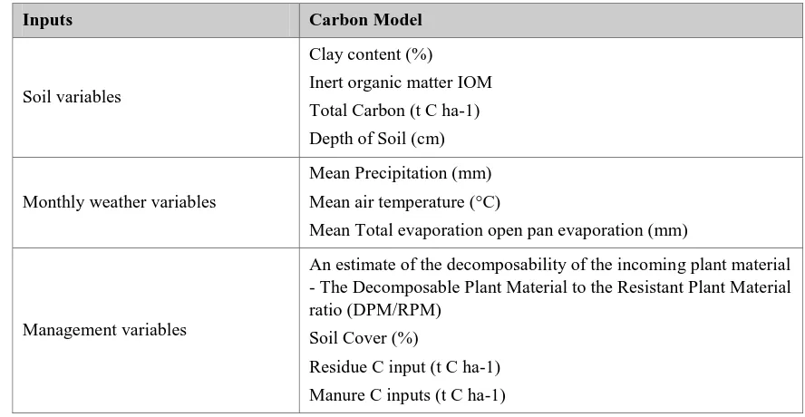
[image:37.595.101.545.363.593.2]3.2.5Required model inputs
Table 2 - The major input variables for the RothC model
Inputs Carbon Model
Soil variables
Clay content (%) Inert organic matter IOM Total Carbon (t C ha-1) Depth of Soil (cm)
Monthly weather variables
Mean Precipitation (mm) Mean air temperature (°C)
Mean Total evaporation open pan evaporation (mm)
Management variables
An estimate of the decomposability of the incoming plant material - The Decomposable Plant Material to the Resistant Plant Material ratio (DPM/RPM)
Soil Cover (%)
Residue C input (t C ha-1) Manure C inputs (t C ha-1)
Table 2 provides a list major model variables required for the RothC carbon model.
26
3.3
Input Variables
3.3.1Weather Variables
All of the weather variables were obtained from the Bureau of Metrology's Climate Web Site (BOM 2011c, 2011b, 2011a).
The rainfall and temperature data is publicly available for average monthly conditions, these values were averaged over the period 1961 to 1990. The monthly data for rainfall is determined by summing the monthly rainfall totals and dividing by the number of years within the period (BOM 2011c, 2011a). The data for rainfall and temperature was available for each month in the format of a two-dimensional, ortho-rectified array of text with a grid size 0.025°/2.5 km.
Evaporation data was required as pan evaporation, this data is publicly available for average monthly conditions, averaged over the period 1975 to 2005. The evaporation data is was available for download in a similar format, however this data was only available with an increased grid size of 0.25°/25 km (BOM 2011b).
Once obtained this data was processed in arcGIS, by converting it to a raster image (*.tiff format) using the ASCII to Raster tool. Once converted, the rainfall, temperature, and evaporation rasters were loaded into the working ArcGIS map file.
3.3.2Soil Variables
The soil variables required were Clay content (%), IOM, Total Carbon (t C ha-1) and Depth of Soil (cm). Clay content (%) and IOM were required to be estimated. Point data for Total Carbon (t C ha-1) was acquired from other studies (Gray et al. 2008 ; Lawrie 2012), the results of these studies also determined the depth of soil used and this was 10cm.
Experimental Data
The experimental soils data utilised for this study was obtained from the following two studies;
Soil Condition and Land Management within Capability 2008 baseline project by the Department of Environment, Climate Change and Water (Gray et al. 2008 ) , this data is referred to as the MER data; and
CarbonWatch program, 2012 undertaken by HHM Projects (Lawrie 2012).
27 Both of these studies are unpublished, however both studies used a randomised sampling technique and the selected sites were chosen to be representative of the local areas dominate features.
The relevant data from the above studies included the position (Easting, Northing MGA or Lat/Long GDA), TOC (% Carbon), bulk density (g/cm3), field texture and land use. The position of the sampled soil was obtained using a hand held GPS. TOC in both studies was obtained by the Leco combustion method. Bulk density was obtained by weighing a known volume of each sample. The known volume was obtained by using 5cm or 10cm lengths of a 40mm or 50mm diameter core. Field textures were determined through the nature and feel of the soil bolus this process is described in (Isbell 1996). Finally the land use was noted in terms of following classifications; Unimproved pastures, improved pastures, cropping and horticulture, national park, forestry or unused. From the above results TOC was converted to tones carbon per hectare by:
20
10000 %
3 1
5
bulkdensity gcm TOC Carbon
ha tC TOCtop cm
(1.10) The carbon content was corrected for gravel (soil particles greater than 2mm) through multiplying TOC by the lost percentage of gravel, (1 - %gravel), as this proportion of the soil is removed prior to carbon content analysis but included in the bulk density analysis.
Both of the above studies included a larger study area than that of this study, the extent of which is shown in Figure 4. As such only the results from data that fell within the study area of are presented for review of model fit in the results. However there was a need to utilise sample locations that fell outside of the study to have sufficient points to initialise the model and calculate IOM. Sample locations outside the study area were only used where the climate was similar to the study area and clay content was known. The climate was assessed as similar through visually reviewing rainfall and topographical locations.
Determined Variables
As the soil samples only represent a small proportion of the overall study area, and as it is impractical to sample all areas within the modelled area, this study estimated the required model parameters outside of the sampled locations by the following methods. These estimated values were then compared with the experimentally measured variables.
28
and the distribution of the (DPM/RPM) ratio. Therefore these properties are required to be determined before soil carbon can be assessed on a regional scale.
Percentage Clay
A soils percentage clay is highly variable; soil clay content is a function of topography, parent material, climate, biota and time (Singer & Munns 2006) and could be any value between 0 and 100%. Therefore any estimate is expected to be poor, however the method by which the clay content was estimated for this study was using topography and mapped soils landscape maps.
This study area falls within the mapped Singleton soils landscape region (Kovac & Lawrie 1990). The Soil Landscape Survey for the Singleton area was produced as part of a state wide mapping program. Soil landscapes are units that have recognisable topography's and soils. Soil landscapes provide broad information on soil occurrences and characteristics and have been produced using aerial photography, field observations and correlation to previously mapped geology or geomorphological features, landform patterns, vegetation, climate and drainage (Kovac & Lawrie 1990).
[image:40.595.147.388.439.647.2]This map describes the expected soils within and the area and describes them in terms of soil dominance, slope and expected location within a topographical sequence. This study utilises a combination of slopes and the relative area of the slope and compares that to the dominance of an expected soil within a landscape to estimate the expected soil type and therefore expected texture class. For the purpose of this study percentage clay was estimated as the centroid of the soil textures class as presented in the Figure 7.
Figure 7 - Triangle texture diagram (Marshall 1947)
29
Tabl