C
2011. The American Astronomical Society. All rights reserved. Printed in the U.S.A.
KEPLER-10 c: A 2.2 EARTH RADIUS TRANSITING PLANET IN A MULTIPLE SYSTEM
Fran¸cois Fressin1, Guillermo Torres1, Jean-Michel D´esert1, David Charbonneau1, Natalie M. Batalha2, Jonathan J. Fortney3, Jason F. Rowe4,17, Christopher Allen4,5, William J. Borucki4, Timothy M. Brown6,
Stephen T. Bryson4, David R. Ciardi7, William D. Cochran8, Drake Deming9, Edward W. Dunham10,
Daniel C. Fabrycky3, Thomas N. Gautier III11, Ronald L. Gilliland12, Christopher E. Henze4, Matthew J. Holman1, Steve B. Howell13, Jon M. Jenkins4,14, Karen Kinemuchi4,15, Heather Knutson16, David G. Koch7,
David W. Latham1, Jack J. Lissauer4, Geoffrey W. Marcy16, Darin Ragozzine1, Dimitar D. Sasselov1, Martin Still4,15, Peter Tenenbaum4,5, and Kamal Uddin4,5
1Harvard-Smithsonian Center for Astrophysics, Cambridge, MA 02138, USA;[email protected] 2Department of Physics, San Jose State University, San Jose, CA 95192, USA
3Department of Astronomy and Astrophysics, University of California, Santa Cruz, CA 95064, USA 4NASA Ames Research Center, Moffett Field, CA 94035, USA
5Uddin Orbital Sciences Corporation, Moffett Field, CA 94035, USA 6Las Cumbres Observatory Global Telescope, Goleta, CA 93117, USA 7NASA Exoplanet Science Institute/Caltech, Pasadena, CA 91125, USA 8McDonald Observatory, University of Texas at Austin, Austin, TX 78712, USA
9NASA Goddard Space Flight Center, Greenbelt, MD 20771, USA 10Lowell Observatory, Flagstaff, AZ 86001, USA
11Jet Propulsion Laboratory/California Institute of Technology, Pasadena, CA 91109, USA 12Space Telescope Science Institute, Baltimore, MD 21218, USA
13National Optical Astronomy Observatory, Tucson, AZ 85719, USA 14SETI Institute/NASA Ames Research Center, Moffett Field, CA 94035, USA
15Bay Area Environmental Research Institute, Sonoma, CA 95476, USA 16Astronomy Department, University of California, Berkeley, CA 94720, USA
Received 2011 April 9; accepted 2011 April 30; published 2011 October 10
ABSTRACT
The Keplermission has recently announced the discovery of Kepler-10 b, the smallest exoplanet discovered to date and the first rocky planet found by the spacecraft. A second, 45 day period transit-like signal present in the photometry from the first eight months of data could not be confirmed as being caused by a planet at the time of that announcement. Here we apply the light curve modeling technique known asBLENDERto explore the possibility that the signal might be due to an astrophysical false positive (blend). To aid in this analysis we report the observation of two transits with theSpitzer Space Telescopeat 4.5μm. When combined, they yield a transit depth of 344±85 ppm that is consistent with the depth in theKeplerpassband (376±9 ppm, ignoring limb darkening), which rules out blends with an eclipsing binary of a significantly different color than the target. Using these observations along with other constraints from high-resolution imaging and spectroscopy, we are able to exclude the vast majority of possible false positives. We assess the likelihood of the remaining blends, and arrive conservatively at a false alarm rate of 1.6×10⁻⁵that is small enough to validate the candidate as a planet (designated Kepler-10 c) with
a very high level of confidence. The radius of this object is measured to beRp =2.227+0.052−0.057R⊕ (in which the
error includes the uncertainty in the stellar properties), but currently available radial-velocity measurements only place an upper limit on its mass of about 20M⊕. Kepler-10 c represents another example (with Kepler-9 d and Kepler-11 g) of statistical “validation” of a transiting exoplanet, as opposed to the usual “confirmation” that can take place when the Doppler signal is detected or transit timing variations are measured. It is anticipated that many of Kepler’s smaller candidates will receive a similar treatment since dynamical confirmation may be difficult or impractical with the sensitivity of current instrumentation.
Key words: binaries: eclipsing – planetary systems – stars: individual (Kepler-10, KOI-072, KIC 11904151) – stars: statistics
Online-only material:color figures
1. INTRODUCTION
The Kepler mission has recently made public a catalog of all transiting planet candidates identified during the first four months of observation by the spacecraft (Borucki et al. 2011b). Included in this list of 1235 objects are nearly 300 in the category of super-Earths (defined here as having radii in the range 1.25R⊕ < Rp < 2R⊕), and several dozen of
Earth-size (Rp < 1.25R⊕). The wealth of new information
17NASA Postdoctoral Program Fellow.
than 2R⊕ with orbital periods up to 50 days (A. W. Howard et al.2011, in preparation), among others.
For good reasons the confirmation or “validation” of small transiting planets18(Earth-size or super-Earth-size) has attracted considerable attention, but has proven to be non-trivial in many cases because of the difficulty of detecting the tiny radial-velocity (RV) signatures that these objects cause on their parent stars, as exemplified by the cases of CoRoT-7 b (L´eger et al. 2009), Kepler-9 d (Torres et al.2011), and Kepler-11 g (Lissauer et al.2011a). In fact, such spectroscopic signals are often too small to detect with current instrumentation, and the planetary nature of the candidate must be established statistically, as in the latter two cases.
The smallest planet discovered to date, Kepler-10 b, was announced recently by Batalha et al. (2011), and is the Kepler mission’s first rocky planet. It has a measured ra-dius of 1.416+0.033
−0.036R⊕ and a mass of 4.6+1.2−1.3M⊕, leading
to a mean density of 8.8+2.1
−2.9g cm−3 which implies a
signifi-cant iron mass fraction (Batalha et al. 2011). Its parent star, Kepler-10 (KIC 11904151, 2MASS 119024305+5014286), is relatively bright among theKepler targets (Keplermagnitude Kp=10.96) and displaystwoperiodic signals with periods of 0.84 days and 45.3 days, and flux decrements (ignoring limb darkening) of 152±4 ppm and 376±9 ppm, respectively (Batalha et al.2011). The extensive observations that followed the detection of these signals are documented in detail by those authors, and include the difficult measurement of the reflex RV motion of the star with a semi-amplitude of only 3.3+0.8−1.0m s−1
and a period that is consistent with the shorter signal. As is customary also in ground-based searches for transiting planets, the shapes of the spectral lines were examined carefully to rule out changes of similar amplitude correlating with orbital phase that might indicate a false positive, such as a background eclips-ing binary (EB) blended with the target, or an EB physically associated with it. However, the precision of the measurements (bisector spans) compared to the small RV amplitude did not al-low such changes to be ruled out unambiguously. False positive scenarios were explored with the aid ofBLENDER, a technique that models the transit light curves to test a wide range of blend configurations (Torres et al. 2011), and it was found that the overwhelming majority of them can be rejected. This and other evidence presented by Batalha et al. (2011) allowed the plan-etary nature of Kepler-10 b to be established with very high confidence.
This was not the case, however, for the 45 day period signal referred to as KOI-072.02 (Kepler Object of Interest 72.02), which is the subject of this paper. No significant RV signal was detected at this period, and only an upper limit on its amplitude could be placed. Using BLENDER, Batalha et al. (2011) were able to rule out a large fraction of the blend scenarios involving circular orbits (including hierarchical triples), but eccentric orbits were not explored because of the increased complexity of the problem and the much larger space of parameters for false positives. While circular orbits are a reasonable assumption for Kepler-10 b because of the strong effects of tidal forces at close range, this is not true for KOI-072.02 on account of its much longer orbital period (see, e.g., Mazeh2008); eccentric orbits cannot be ruled out.
18 In the context of this paper “confirmation” refers to the unambiguous
detection of the gravitational influence of the planet on its host star or on other bodies in the system (e.g., the Doppler signal or transit timing variations) to establish the planetary nature of the candidate; when this is not possible, we speak of “validation,” which involves an estimate of the false alarm probability.
This provides the motivation for the present work, in which we set out to examine all viable astrophysical false positive sce-narios for KOI-072.02 with the goal of validating it as a bona fide planet. In addition to improvements in theBLENDER mod-eling, we bring to bear new near-infrared observations obtained with theSpitzer Space Telescopein which the transits are clearly detected as well as the complete arsenal of follow-up observa-tions gathered by the Kepler team, including high-resolution adaptive optics (AO) imaging and speckle interferometry, high-resolution spectroscopy, and an analysis based on the Kepler observations themselves of the difference images in and out of transit for positional displacements (centroid motion). All of these observations combined with the strong constraints pro-vided by BLENDERsignificantly limit the kinds of blends that remain possible, and as we describe below they allow us to claim with very high confidence that KOI-072.02 is indeed a planet. Its estimated radius is approximately 60% of that of Neptune. With this, Kepler-10 becomes the mission’s third confirmed multi-planet system (after Kepler-9 and Kepler-11; Holman et al. 2010; Lissauer et al.2011a) containing a tran-siting super-Earth-size planet and at least one larger planet that also transits.
We begin with a brief recapitulation of theBLENDER tech-nique, including recent improvements. We then present the Warm Spitzerobservations at 4.5μm that help rule out many blends, and we summarize additional constraints available from other observations. This is followed by the application of BLENDERto KOI-072.02 in order to identify all blend scenarios that can mimic the Kepler transit light curve. Next we com-bine this information with the other constraints and carry out a statistical assessment of the false alarm rate (FAR) for the planet hypothesis, leading to the validation of the candidate as Kepler-10 c. We conclude with a discussion of the possible con-stitution of the new planet in the light of current models, and the significance of this type of validation.
2. REJECTING FALSE POSITIVES WITHBLENDER
The detailed morphology of a transit light curve (length of ingress/egress, total duration) contains important information that can be used to reject many false positive scenarios, produc-ing brightness variations that do not quite have the right shape even though they may well match the observed transit depth (see, e.g., Snellen et al.2009).BLENDER(Torres et al.2004,2011) takes advantage of this to explore a very large range of sce-narios, including background or foreground eclipsing binaries blended with the target as well as eclipsing binaries physically associated with the target in a hierarchical triple configuration. Following the notation introduced by Torres et al. (2011), the objects composing the binary are referred to as the “secondary” and “tertiary,” and the candidate is the “primary.” The tertiary can be either a star (including a white dwarf) or a planet, and the secondary can be a main-sequence star or a (background) giant. With the help of model isochrones to set the stellar properties, BLENDERsimulates blend light curves resulting from the flux of the eclipsing pair diluted by the brighter target (and any addi-tional stars that may fall within the photometric aperture). Each simulated light curve is compared with theKeplerobservations in aχ2sense to identify which of them result in acceptable fits (to
be defined later). The parameters varied during the simulations are the mass of the secondary star (M2), the mass of the tertiary
(M3, or its radiusR3if a planet), the impact parameter (b), the
to the duration for a circular orbit (see below). For convenience, the relative linear distance is parameterized in terms of the dif-ference in distance modulus,Δδ, whereΔδ =5 log(dEB/dKOI).
In the case of hierarchical triple configurations, the isochrone for the binary is assumed to be the same as for the primary (metallicity of [Fe/H]= −0.15 and a nominal age of 11.9 Gyr; see Batalha et al.2011), whereas for background blends we have adopted for the binary a representative 3 Gyr isochrone of solar metallicity although these parameters have a minimal impact on the results. For full details of the technique we refer the reader to the references above. Three recent changes and improvements that are especially relevant to the application to KOI-072.02 are described next.
1. The relatively long orbital period of KOI-072.02 (45.3 days) precludes us from assuming that the eccentricity (e) is zero, as we were able to suppose in previous applications of BLENDERto Kepler-9 d and Kepler-10 b, which have periods of 1.59 and 0.84 days, respectively. The reason that matters is that the duration of the transit is set, among other factors, by the size of the secondary star. Eccentricity can alter the speed of the tertiary around the secondary, making it slower or faster than in the circular case depending on the orientation of the orbit (longitude of periastron,ω). Given a fixed (measured) duration, blends with smaller or larger secondary stars than in the circular case may still provide satisfactory fits to the light curve, effectively increasing the pool of potential false positives.
BLENDERnow takes this into account, although rather than usingeandω, which are the natural variables employed in the binary light curve generating routine at the core of BLENDER(see Torres et al. 2011) as parameters, a more convenient variable that captures the effects of both is the duration relative to a circular orbit. Following Winn (2010), this may be expressed asD/Dcirc≈
√
1−e2/(1 +esinω).
Operationally, then, we varyD/Dcircover wide ranges as we explore different blend scenarios, and for each value, we infer the corresponding values ofeandω. In practice, in order to solve for {e, ω} from D/Dcirc it is only
necessary to consider the limiting cases with ω = 90◦ and 270◦, corresponding to transits occurring at periastron and apastron, respectively, since these are the orientations resulting in the minimum and maximum durations for a given eccentricity. Other combinations ofeandωwill lead to intermediate relative durations that are already sampled in our D/Dcirc grid. It is worth noting that use of only
these two values ofωleads to predicted secondary eclipses in the simulated light curves that are always located at phase 0.5, whereas secondary eclipses in the real data might be present at any phase. For our purposes, this is of no consequence, as KOI-072.02 has already had its light curve screened for secondary eclipses at any phase that might betray a false positive as part of the vetting process. No such features are present down to the 100 ppm level. Thus, any simulated light curves fromBLENDER that display a significant secondary eclipse will yield poor fits no matter where the secondary eclipse happens to be, and will lead to the rejection of that particular blend scenario.
2. For each false positive configurationBLENDERcan predict the overall photometric color of the blend, for comparison with the measured color index of the candidate as reported in theKeplerInput Catalog (KIC; Brown et al. 2011). A color index such as Kp−Ks, where Kp is the Kepler
magnitude and Ks is derived from the Two Micron All
Sky Survey catalog, provides a reasonable compromise between wavelength leverage and the precision of the index. The latter varies typically between 0.015 and 0.030 mag depending on the passband and the brightness of the star (see Brown et al.2011). We consider a particular blend to be rejected when its predicted color deviates from the KIC value by more than three times the error of the latter. As it turns out, color is a particularly effective way of rejecting blends that include secondary stars of a different spectral type than the primary, such as those that become possible when allowing for eccentric orbits.
3. Recent refinements in the resolution of theBLENDER simu-lations to better explore parameter space, in addition to the inclusion of eccentricity (orD/Dcirc) as an extra variable,
have increased the complexity of the problem as well as the computing time (by nearly two orders of magnitude) compared to the relatively simple case of circular orbits. The number of different parameter combinations examined withBLENDER(and corresponding light curve fits) can ap-proach 7×10⁸in some cases. Consequently, the simulations
are now performed on the Pleiades cluster at the NASA Advanced Supercomputing Division, located at the Ames Research Center (California), typically on 1024 processors running in parallel. For convenience hierarchical triple con-figurations (four parameters) and background/foreground blends (five parameters) are studied separately, each for the two separate cases of stellar and planetary tertiaries (for a total of four grids). One additional fit is carried out using a true transiting planet model to provide a reference for the quality of the false positive fits in the other grids.
The discriminating value of the shape information contained in the light curves, mentioned at the beginning of this section, is highlighted by ourBLENDERresults for Kepler-10 b, as de-scribed by Batalha et al. (2011). In that study it was found thatall background EB configurations with stellar tertiaries yield very poor fits to theKeplerlight curve and are easily rejected. The underlying reason is that all such blend models predict obvious brightness changes out of eclipse (ellipsoidal variations) with an amplitude that is not seen in the data, and which are a con-sequence of the very short orbital period.19 Hierarchical triple scenarios were also excluded based on joint constraints from BLENDERand other follow-up observations. The only configu-rations providing suitable alternatives to the true planet scenario involved stars in the foreground or background of the target that are orbited by a larger transiting planet. The considerable re-duction in the blend frequency (BF) from the exclusion of all background eclipsing binaries led to a false alarm probability low enough to validate Kepler-10 b with a very high level of confidence,independentlyof any spectroscopic evidence. This remarkable result speaks to the power ofBLENDERwhen com-bined with all other observational constraints. It also assumes considerable significance for Kepler-10 b, given that it was not
19 Note that the present post-processing ofKeplerdata in preparation for the
possible to provide separate proof of the planetary nature of this signal in the Batalha et al. (2011) study from an exami-nation of the bisector spans. The scatter of the bisector span measurements (10.5 m s−1) was three times larger than the RV
semi-amplitude (3.3 m s−1), rendering them inconclusive. The situation regarding theBLENDER analysis of the KOI-072.02 signal in the Batalha et al. (2011) study was very different: the orbital period is much longer, and ellipsoidal variations are predicted to be negligible, so that background eclipsing binaries with stellar tertiaries remain viable blends. This, and the added complication from eccentric orbits, hindered the efforts of those authors to validate this candidate. With the benefit of the enhancements inBLENDERdescribed above, we are now in a better position to approach this problem anew.
As follow-up observations provide important constraints that are complementary to those supplied by BLENDER, and play an important role in determining the FAR for the planetary nature of KOI-072.02 (Section6), we describe those first below, beginning with our new near-infraredSpitzerobservations.
3. OBSERVATIONAL CONSTRAINTS
3.1. Warm Spitzer Observations of KOI-072.02
KOI-072.02 was observed during two transits with the IRAC instrument on the Spitzer Space Telescope (Werner et al. 2004; Fazio et al. 2004) at 4.5 μm (program ID 60028). The observations were obtained on UT 2010 August 30 and November 15, with each visit lasting approximately 15 hr 10 minutes. The data were gathered in full-frame mode (256× 256 pixels) with an exposure time of 6.0 s per image, which resulted in approximately a 7.1 s cadence and yielded 7700 images per visit.
The method we used to produce photometric time series from the images is described by D´esert et al. (2009). It consists of finding the centroid position of the stellar point-spread function (PSF) and performing aperture photometry using a circular aperture on individual exposures. The images used are the Basic Calibrated Data delivered by theSpitzerarchive. These files are corrected for dark current, flat fielding, and detector nonlinearity, and are converted to flux units. We converted the pixel intensities to electrons using the information on the detector gain and exposure time provided in the FITS headers. This facilitates the evaluation of the photometric errors. We extracted the UTC-based Julian date for each image from the FITS header (keyword DATE_OBS) and corrected to mid-exposure. We converted to TDB-based barycentric Julian dates using theUTC2BJD20 procedure developed by Eastman et al. (2010). This program uses the JPL Horizons ephemeris to estimate the position of the Spitzer spacecraft during the observations. We then corrected for transient pixels in each individual image using a 20 point sliding median filter of the pixel intensity versus time. To do so, we compared each pixel’s intensity to the median of the 10 preceding and 10 following exposures at the same pixel position, and we replaced outliers greater than 4σ with their median value. The fraction of all pixels we corrected is 0.02% for the first visit and 0.06% for the second.
The centroid position of the stellar PSF was determined using the DAOPHOT-related proceduresGCNTRD, from the IDL Astronomy Library.21 We applied theAPERroutine to perform
20 http://astroutils.astronomy.ohio-state.edu/time/ 21 http://idlastro.gsfc.nasa.gov/homepage.html
aperture photometry with a circular aperture of variable radius, using a range of radii between 1.5 and 8 pixels in steps of 0.5. The propagated uncertainties were derived as a function of the aperture radius, and we adopted the aperture providing the smallest errors. We found that the transit depths and errors varied only weakly with aperture radius for all light curves analyzed in this project. The optimal aperture was found to have a radius of 4.0 pixels.
We estimated the background by examining a histogram of counts from the full array. We fit a Gaussian curve to the central region of this distribution (ignoring bins with high counts, which correspond to pixels containing stars), and we adopted the center of this Gaussian as the value of the residual background intensity. As seen already in previous WarmSpitzerobservations (Deming et al. 2011; Beerer et al. 2011), we found that the background varies by 20% between three distinct levels from image to image, and displays a ramp-like behavior as function of time. The contribution of the background to the total flux from the stars is low for both observations, from 0.1% to 0.55% depending on the image. Therefore, photometric errors are not dominated by fluctuations in the background. We used a sliding median filter to select and trim outliers in flux and position greater than 5σ, representing 1.6% and 1.3% of the data for the first and second visits, respectively. We also discarded the first half-hour’s worth of observations, which is affected by significant telescope jitter before stabilization. The final number of photometric measurements used is 7277 and 7362.
The raw time series are presented in the top panel of Figure1. We find that the point-to-point scatter in the photometry gives a typical signal-to-noise ratio (S/N) of 280 per image, which corresponds to 90% of the theoretical S/N. Therefore, the noise is dominated by Poisson statistics.
3.2. Analysis of the Warm Spitzer Light Curves and Results
In order to determine the transit parameters and associated uncertainties from theSpitzertime series we used a transit light curve model multiplied by instrumental decorrelation functions, as described by D´esert et al. (2011a). The transit light curves were computed with the IDL transit routineOCCULTSMALLfrom Mandel & Agol (2002). For the present case we allowed for a single free parameter in the model, which is the planet-to-star radius ratioRp/R(or equivalently, the depth, in the absence of
limb darkening). The normalized orbital semimajor axis (system scale)a/R, the impact parameterb, the periodP, and the time
of mid-transit Tc were held fixed at the values derived from
the Kepler light curve, as reported by Batalha et al. (2011) and summarized below in Section7. Limb darkening is small at 4.5μm, but was nevertheless included in our modeling using the four-parameter law by Claret (2000) and theoretical coefficients published by Sing (2010).
Figure 1.Spitzertransit light curves of KOI-072.02 observed in the IRAC bandpass at 4.5μm. Top: raw measurements (black points) with the same data binned by two superimposed (12 s bins, red points). Bottom: measurements combined from the two visits and binned in 36 minute bins (295 points per bin), along with the best-fit limb-darkened transit model (integrated over the same duration). Both the data and the model shown here have been corrected for instrumental errors. (A color version of this figure is available in the online journal.)
transit and instrumental model parameters (seven in total). The errors on each photometric point were assumed to be identical and were set to the rms residual of the initial best fit. To obtain an estimate of the correlated and systematic errors in our mea-surements (Pont et al.2006) we used the residual permutation bootstrap technique, or “Prayer Bead” method, as described by D´esert et al. (2009). In this method the residuals of the ini-tial fit are shifted systematically and sequenini-tially by one frame, and then added to the transit light curve model before fitting again. We considered asymmetric error bars spanning 34% of the points above and below the median of the distributions to derive the 1σ uncertainties for each parameter, as described by D´esert et al. (2011b).
The bottom panel of Figure 1 shows the best-fit model superimposed on the observations from the two visits combined, with the data binned in 36 minute bins for clarity (295 points per bin). The transit depths at 4.5 μm (after removing limb-darkening effects) are 353+115
−133ppm for the first visit and 339+85−110
for the second, which are in good agreement with each other. The weighted average depth of 344±85 is consistent with the non-limb-darkened value of 376±9 ppm derived from the Keplerlight curve (Batalha et al.2011) well within the 1σerrors, strongly suggesting the transit is achromatic, as expected for a planet.
The aboveSpitzerobservations provide a useful constraint on the kinds of false positives (blends) that may be mimicking the KOI-072.02 signal. For example, if Kepler-10 were blended with a faint unresolved background EB of much later spectral type that manages to reproduce the transit depth in theKepler passband, the predicted depth at 4.5μm may be expected to be larger because of the higher flux of the contaminating binary at longer wavelengths compared to Kepler-10. Since the transit depth we measure in the near-infrared is about the same as in the optical, this argues against blends composed of stars of much later spectral type. Based on model isochrones and the properties
of the target star (see below), we determine an upper limit to the secondary masses of 0.77M. ThisSpitzerconstraint is used in Section4to eliminate many blends.
3.3. Additional Observational Constraints on Possible False Positives
Further constraints of a different kind are provided by high-resolution imaging as described in more detail by Batalha et al. (2011). Briefly, these consist of speckle observations obtained on UT 2010 June 18 with a two-color (approximatelyVandR) speckle camera on the WIYN 3.5 m telescope on Kitt Peak (see Howell et al.2011), and near-infrared (J-band) AO observations conducted on UT 2009 September 8 with the PHARO camera on the 5 m Palomar telescope. No companions were detected around Kepler-10 within 1.5 (for speckle) or 12.5 (AO), and more generally these observations place strong limits on the presence of other stars as a function of angular separation (down to 0.05 in the case of speckle) and relative brightness (companions as faint asΔJ = 9.5 for AO). These sensitivity curves are shown in Figure 9 of Batalha et al. (2011), and we make use of that information below.
High-resolution spectra described also by Batalha et al. (2011) and obtained with the HIRES instrument on the 10 m Keck I telescope place additional limits on the presence of close companions falling within the spectrograph slit (0.87), such that stars within about 2 mag of the target would generally have been seen. A small chance remains that these companions could escape detection if their RV happens to be within a few km s−1 of that of the target (which is a narrow-lined, slowly
motions. We explored this through Monte Carlo simulations. The results indicate that the probability of having a physical companion within a conservative range of±10 km s−1 of the RV of the target that would also go unnoticed in our speckle observations, and that additionally would not induce a RV drift on the target large enough to have been detected in the high-precision measurements of Batalha et al. (2011), is only about 0.1%.
Finally, an analysis of the image centroids measured from the Kepler observations rules out background objects of any brightness beyond about 2 of the target. This exclusion limit (equivalent to half a pixel) is considerably more conservative than the 0.6 reported by Batalha et al. (2011), and accounts for saturation effects not considered earlier (given that atKp = 10.96 the star is very bright by Kepler standards) as well as quarter-to-quarter variations (where “quarters” usually represent three-month observing blocks interrupted by spacecraft rolls required to maintain the proper illumination of the solar panels).
4. APPLICATION OFBLENDERTO KOI-072.02
TheKeplerphotometry used here is the same as employed in the work of Batalha et al. (2011) and was collected between 2009 May 2 and 2010 January 9. These dates correspond toKepler Quarter 0 (first nine days of commissioning data) through the first month of Quarter 4. For this study we used only the long-cadence observations (10,870 measurements) obtained by the spacecraft at regular intervals of about 29.4 minutes. All blend models generated withBLENDERwere integrated over this time interval for comparison with the measurements. The original data have been de-trended for this work by removing a first-order polynomial, and then applying median filtering with a two-day wide sliding window. Observations that occur during transits were masked and did not contribute to the median calculation. Because this sliding window is considerably shorter than the 45.3 day orbital period, any ellipsoidal variations present in the original data should be largely preserved, although in any case they are expected to be very small for binaries with periods as long as this. We adopted also the ephemeris of mid-transit for KOI-072.02 as reported by Batalha et al. (2011), which isTc[BJD] = 2,454,971.6761 +N ×45.29485 days,
whereNis the number of cycles from the reference epoch. Because it is relatively bright (Kp = 10.96), Kepler-10 was also observed by the mission with a shorter cadence of approximately 1 minute for a period of several months to allow an asteroseismic characterization of the star. A total of 19 oscillation frequencies were detected, and enabled a very precise determination of the mean stellar density. When combined with stellar evolution models and a spectroscopic determination of the effective temperature and chemical composition, the resulting parameters for the star are very well determined. Kepler-10 is relatively old (>7.4 Gyr) but is otherwise quite similar to the Sun, with a temperature ofTeff =5627±44 K,
a mass and radius of M = 0.895 ±0.060 M and R =
1.056±0.021R, and a composition [Fe/H]= −0.15±0.06 slightly below solar (Batalha et al.2011).
As indicated earlier we considered four general sce-narios for false positives: chance alignments (a pair of background/foreground eclipsing objects) and hierarchical triple systems, each with tertiaries that can be either stars or planets. The free parameters were varied over the following ranges: secondary massM2between 0.10 and 1.40M, in steps
of 0.02M; tertiary massM3 between 0.10 and M2, also in
steps of 0.02M; tertiary radiusR3between 0.06 and 2.00RJup
in steps of 0.02RJup; impact parameterbbetween 0.00 and 1.00
in steps of 0.05; relative durationD/Dcircbetween 0.2 and 4.6 in steps of 0.2, corresponding to eccentricities up to 0.92 and values ofωof 90◦and 270◦ (see Section2); and relative dis-tanceΔδ(distance modulus difference) between−5.0 and +9.0 in steps of 0.5 mag, except for hierarchical triple configurations, for whichΔδ=0.
The goodness of the fit of each of the large number of synthetic light curves generated byBLENDERis quantified here by computing the χ2 statistic and comparing it with that of the best planet model fit. The difference can be assigned a significance level (or FAR) that depends on the number of free parameters of the problem. For example, for a blend scenario corresponding to a hierarchical triple system (4 degrees of freedom), a trial model giving a worse fit than the planet solution byΔχ2 =4.72 is statistically different at the 1σlevel, assuming
Gaussian errors (see, e.g., Press et al.1992). A fit that is worse by
Δχ2=16.3 is different at the 3σlevel. Hierarchical triple blends
giving poorer fits than this are considered here to be ruled out by the Keplerphotometry. For background/foreground scenarios (5 degrees of freedom) the 3σ blend rejection level isΔχ2 = 18.2.
4.1.BLENDERResults
In this section, we describe the simulations carried out for the four general blend configurations mentioned above. Although the secondaries for the background scenarios can in principle also be evolved stars (giants), as opposed to main-sequence stars, we consistently found that the transit light curves generated by such systems give a very poor match to the observations because they do not have the right shape (the ingress/egress phases are too long). Therefore, we restricted our exploration of parameter space to main-sequence stars only.
An additional possibility for a false positive may stem from an error in the determination of the orbital period. If the true period were twice the nominal value, alternating transit events would correspond to primary and secondary eclipses, implicating a blended EB. The primary and secondary eclipses would often (but not always) be of different depth. As part of the vetting process for each candidate, the Kepler team examines the even-numbered and odd-numbered events to look for differences in depth that may indicate a false positive of this kind. As described by Batalha et al. (2011), no significant differences were found for KOI-072.02 beyond the 2σ level, whereσ represents the uncertainty in the transit depth (9 ppm). Nevertheless, as the possibility still exists that the components of the EB are identical, experiments were run withBLENDERto examine the transit shape produced by such scenarios, and it was found that the ingress and egress phases are always much too long compared to the observations, as expected for two equal-size stars eclipsing each other. Thus, these scenarios are easily ruled out as well.
4.1.1. Background Eclipsing Binaries (Star+Star)
The simulations withBLENDERindicate that few background blend scenarios with stellar tertiaries are able to mimic the transit features in the light curve at an acceptable level, and they all correspond to somewhat eccentric orbits. In Figure2, we show the goodness of fit of these scenarios, with the small closed 3σ contour representing the region of parameter space within which the fits are satisfactory, according to the criteria given above. Only blends with secondary massesM2larger than about
8.6
+
[image:7.612.320.565.52.288.2]2.5 2.5
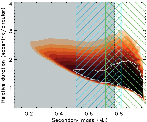
Figure 2.Map of theχ2surface (goodness of fit) corresponding to a grid of blend
models for KOI-072.02 involving background eclipsing binaries. The linear separation between the binary and the primary is cast in terms of the distance modulus difference. Contours are drawn as a function of theχ2difference from
the best planet model fit (expressed in units of the significance level of the difference,σ), and are plotted here as a function of the mass of the secondary star. Only blends within the small white contour yield acceptable fits to the light curve (within 3σ of the planet fit). Other colored areas correspond to regions of parameter space giving increasingly worse fits (4σ, 5σ, etc.), representing blends we consider to be ruled out. TheSpitzerconstraint is indicated by the shaded area: blends with secondary masses in this region are excluded (see Section3.2), althoughBLENDERitself already rules out all of these scenarios. Green lines running diagonally from the lower left to the upper right are labeled with the magnitude differenceΔKpof the blended binary relative to the target star. The hatched region below theΔKp=2 mag line represents blends with secondary stars bright enough that they would generally be detected in our spectroscopy. Viable blends within the 3σ contour are seen to be confined to a narrow range of magnitude differences (2.5ΔKp3.5, dashed green lines). The dashed line atΔKp =8.6 indicates the envelope for the faintest blends that would be capable of reproducing the measured depth based on simple-minded estimates described in the text. As seen,BLENDERprovides much tighter constraints than this. The cross corresponds to a blend model that gives the fit shown in the bottom panel of Figure3.
(A color version of this figure is available in the online journal.)
range of distances behind the target (4.0 Δδ 4.7) for the dilution effect to be just right, such that the corresponding apparent brightness differenceΔKpis between 2.5 and 3.5 mag (see figure). The best among these blend models (located near the center of the contour) provides a fit that is about 2.1σ worse than a planet model (but still acceptable), and is shown in the top panel of Figure3compared against the planet model. The tertiary stars in these blends are constrained to be very small, between 0.10 and 0.16M.
That most blends involving background eclipsing binaries can be ruled out may appear somewhat surprising and is worth investigating. Indeed, for a given measured transit depthdtran,
a blend can only reproduce the light curve if it contributes at least a fractiondtran of the total flux collected in the Kepler
aperture. Thus, one would expect that binaries as faint as
ΔKp= −2.5 log(dtran)≈8.6 mag relative to the target should
be able to match that amount of dimming if they were totally eclipsed (see, e.g., Morton & Johnson2011), and furthermore, that the measured duration could also be reproduced by a large range of secondary sizes with an appropriate combination of orbital eccentricity andω. Yet we find that no blends fainter than
ΔKp=3.5 give tolerable fits to the light curve (see Figure2). A visual understanding of the underlying reason for this may
Figure 3.Long-cadenceKeplerobservations for KOI-072.02 compared with two different blend models involving background eclipsing binaries (red lines), and shown against the best-fit planet model for reference (black line). All models are integrated over the duration of one cadence (29.4 minutes). Top: the blend model shown is the one giving the best fit for this type of scenario (2.1σdifference compared to the planet fit). Bottom: example of a blend model (indicated with a cross in Figure2) that illustrates the use of shape information byBLENDERin a case that would naively be expected to be a viable false positive scenario (see the text). This particular scenario corresponds to a secondary mass ofM2 =1.0Mand a distance modulus difference of 5 mag relative to the target, giving a brightness difference in theKpband of 5.6 mag. Although it matches the depth and total duration of the transit, the ingress and egress phases are not well reproduced, so that the overall quality of the fit is poor and the blend is ruled out at more than the 10σlevel.
(A color version of this figure is available in the online journal.)
be seen in the bottom panel of Figure3, in which we show a blend model that one would naively expect should be able to match the observations, according to the crude recipe described above. This particular blend scenario is marked with a cross in Figure 2, and corresponds toΔδ = 5 andM2 = 1.0 M, resulting in a magnitude difference ofΔKp =5.6 for the EB relative to the target. While this model does yield a good match to the measured depth, and even the total duration, it does not perform nearly as well in the ingress/egress phases, which are too long when compared against the observations. The quality of this fit relative to the best planet fit, which can also be seen in the figure, corresponds to a 10.1σ difference, and therefore BLENDER rejects it. Thus, the reason that most blends of this class can be ruled out is ultimately the high precision of the Keplerlight curves, which provides a very strong constraint on the shape of the transit light curve, and in particular on the size ratio between the secondary and tertiary, which sets the duration of the ingress and egress phases.
4.1.2. Background/Foreground Star+Planet Pairs
[image:7.612.46.291.55.256.2]Allowed Region
Figure 4. Similar to Figure 2, for blends involving background systems consisting of a star transited by a planet. The color scheme is the same as in Figure2. Blends giving fits no worse than 3σfrom the best planet fit are below the thick white contour labeled with that confidence level. The shaded left-hand side of the diagram corresponds to secondary masses excluded by constraints from theSpitzerobservations. Lines of constant magnitude difference relative to the target are shown in green, running diagonally from the lower left to the upper right. The dashed one at the top represents the boundary for the faintest viable blends (tangent to the white 3σcontour). The solid green line below and parallel to it (ΔKp=2 mag) and hatched region to the right marks the area of parameter space excluded by our spectroscopic constraints. The blue curve and hatched region to the left represent blends that are excluded because they are too red inKp−Ks compared to the target. Note that the colors of the
blended stars are computed from a different isochrone than that of the target, which explains why blends with secondaries of the same mass as the target are ruled out for being too red. The combination of all these constraints leaves only a reduced area of parameter space (labeled “Allowed Region”) where blend models give tolerable fits to theKeplerlight curve and are not ruled out by any of our follow-up observations.
(A color version of this figure is available in the online journal.)
below eliminate a substantial fraction of them. All of these blends involve secondary+tertiary pairs that are within 4 mag of the target in theKeplerpassband (diagonal dashed line in the figure). The tertiary sizes in these blends range from 0.42RJup
to 1.84RJup.
Our Warm Spitzer observations set a lower limit of about 0.77Mfor the secondary masses of these blends, as described earlier; scenarios involving redder stars would result in transits at 4.5μm significantly deeper than we observe (i.e., deeper than the measured depth + 3σ). This exclusion region is indicated by the shaded area. Additionally, blends that are much brighter than ΔKp = 2 would most likely have been detected spectroscopically (see Batalha et al. 2011), so we consider those to be ruled out as well. We indicate this with the green hatched region in the lower right-hand side of the figure. Finally, the colors of the background/foreground configurations simulated withBLENDERprovide a further constraint which is represented by the blue hatched area on the lower left of the figure. This swath of parameter space is excluded because the blends are significantly redder than the color index measured for Kepler-10 (Kp−Ks = 1.465 ±0.029), by more than
three times the uncertainty in the observed index. As a result of these complementary constraints, the only section of parameter space remaining for viable blends involving star+planet pairs is the area under the 3σcontour and limited from below and on the left by the hatched areas (color and brightness conditions) and shaded area (Spitzerconstraint), respectively. All of these blends
Figure 5.Similar to Figure2, for the case of hierarchical triple systems in which the secondary star is transited by a planet. The color scheme is the same as in Figure2. In this case the vertical axis shows the tertiary sizes. The constraints fromSpitzer(gray shaded area to the left of 0.77M), color information (blue hatched area on the left), and spectroscopy (green hatched area on the right) are shown as in previous figures. When taken together these constraints eliminate all blends of this kind.
(A color version of this figure is available in the online journal.)
have the eclipsing pair behind the target (foreground scenarios are all ruled out).
We note that in this star+planet blend scenario, white dwarfs can also act as tertiaries as long as they are cooler than the secondaries so that they do not lead to deep occultation events that would have been seen in the light curve of KOI-072.02. The above range of tertiary radii (0.42RJupto 1.84RJup) excludes
essentially all cool carbon–oxygen and oxygen–neon white dwarfs more massive than about 0.4M, as these are smaller than the lower limit set by BLENDER, which corresponds to 4.7 R⊕ (see, e.g., Panei et al. 2000). Low-mass helium-core or oxygen-core white dwarfs that are the product of common-envelope evolution in binary stars can be considerably larger in size, although they appear to be very rare. TheKeplermission itself has uncovered only three examples to date (Rowe et al. 2010; Carter et al. 2011); however, all of them are very hot (Teff > 10,000 K) and produce deep and unmistakable flat-bottomed occultation signals. Model calculations such as those of Panei et al. (2007) show that as these helium-core white dwarfs cool, their radii quickly become Earth-size or smaller. Therefore, we do not consider white dwarfs to be a significant source of blends for KOI-072.02.
4.1.3. Hierarchical Triple Scenarios (Star+Star and Star+Planet Blends)
[image:8.612.45.292.56.249.2]Figure 6.Same as Figure5, but with the vertical axis showing the relative transit durations (D/Dcirc).
(A color version of this figure is available in the online journal.)
all of these blends. For example, the shaded area of parameter space to the left of 0.77M is eliminated by theSpitzer ob-servations, as described earlier. The constraint on theKp−Ks
color (hatched area on the left) is partly redundant with the NIR observations, but extends to slightly larger secondary masses. And finally, the spectroscopic constraint removes the remaining scenarios corresponding to higher-mass (brighter) secondaries. We conclude that of all the hierarchical triple blend scenarios that are capable of precisely reproducing the detailed shape of the Kepler transit light curve, none would have escaped detection by one or more of our follow-up efforts, including NIR Spitzerobservations, high-resolution spectroscopy, or absolute photometry (colors).22 This highlights the importance of these types of constraints for validatingKeplercandidates, given that blends involving physically associated stars would generally be spatially unresolved by our high-resolution imaging with AO or speckle interferometry, and they would typically also be below the sensitivity limits of our centroid motion analysis, so that they would not be detected by those means. Therefore, the only blends we need to be concerned about for KOI-072.02 are those consisting of stars in the background of the target that are orbited by other stars or by transiting planets.
5. A PRIORI LIKELIHOOD OF REMAINING BLEND SCENARIOS FOR KOI-72.02
In order to estimate the frequency of the blend scenarios (i.e., background configurations) that remain possible after applying BLENDER and all other observational constraints, we follow a procedure similar to that described by Torres et al. (2011) for Kepler-9 d. We appeal to the Besan¸con Galactic structure models of Robin et al. (2003) to predict the number density of background stars of each spectral type (mass) and brightness
22 The possibility, remote as it may be, that the target has a physically
associated companion that is nearly of the same brightness and that has managed to elude detection is always present (see Section3.3), not only here but in all previously discovered transiting planets. For the present purposes we do not consider this “twin star” scenario as a false positive in the strict sense (see also Torres et al.2011), as the transiting object would still be a planet, only that it would be larger than we thought by about a factor of√2 because of the extra dilution from the companion.
around Kepler-10, in half-magnitude bins, and we make use of estimates of the frequencies of transiting planets and of eclipsing binaries from recent studies by the Kepler team to infer the number density of blends. Using constraints from our high-resolution imaging (specifically, the sensitivity curves presented by Batalha et al. 2011, their Figure 9) we calculate the area around the target within which blends would go undetected, and with this the expected number of blends.23
The recent release by Borucki et al. (2011b) of a list of 1235 candidate transiting planets (KOIs) fromKeplerprovides a means to estimate planet frequencies needed for our calcula-tions, with significant advantages over the calculations of Torres et al. (2011) for Kepler-9 d, which were based on the earlier list of candidates published by Borucki et al. (2011a). The sample is now not only much larger, but also the knowledge of the rate of false positives for Kepler is much improved, and that rate is believed to be relatively small (20%–40% depending on the level of vetting of the candidate, according to Borucki et al. 2011a; less than 10% according to the recent study by Morton & Johnson2011). Thus, our results will not be significantly af-fected by the assumption that all of the candidates are planets (see also below). An additional assumption we make is that this census is largely complete. Among these candidates we count a total of 267 having radii in the range allowed by BLENDER for the tertiaries of viable blends (i.e., between 0.42 and 1.84RJup). With the total number ofKeplertargets being 156,453
(Borucki et al.2011b), the relevant frequency of transiting plan-ets for our blend calculation isfplanet=267/156,453=0.0017.
Slawson et al. (2011) have recently published a catalog of the 2165 eclipsing binaries found in theKeplerfield, from the first four months of observation. Only the 1225 detached systems among these are considered here, since binaries in the category of semi-detached, overcontact, or ellipsoidal variables would not produce light curves with a shape consistent with a transit. The frequency of eclipsing binaries for our purposes is then fEB=1225/156,453=0.0078.
Table1presents the results of our calculation of the frequency of blends, separately for background blends with stellar tertiaries (eclipsing binaries) and with planetary tertiaries. Columns 1 and 2 give the Kp magnitude range of each bin and the magnitude difference ΔKprelative to the target, calculated at the upper edge of each bin. Column 3 reports the mean number density of stars per square degree obtained from the Besan¸con models, for stars in the mass range allowed by BLENDER as shown in Figure2. In Column 4, we list the maximum angular separationρmaxat which stars in the corresponding magnitude
bin would go undetected in our imaging observations, taken from the information in the work of Batalha et al. (2011). The product of the area implied by this radius and the stellar densities in the previous column give the number of stars in the appropriate mass range, listed in Column 6 in units of 10−6. Multiplying these figures by the frequency of eclipsing binaries fEB then gives the number of background star+star blends in
Column 7. A similar calculation for the background star+planet blends, making use of fplanet, is presented in Columns 7–10.
We sum up the contributions from each magnitude bin at the bottom of Columns 6 and 10. The total number of blends we expect a priori (BF) is given in the last line of the table by adding these two values together, and is BF = 1.62×10⁻⁸.
The calculations show that background blends consisting of
23 In the case of KOI-072.02 the exclusion radius from the centroid motion
Table 1
Blend Frequency Estimate for KOI-072.02
Blends Involving Stellar Tertiaries Blends Involving Planetary Tertiaries
KpRange ΔKp Stellar Densitya ρ
max Stars EBs Stellar Densitya ρmax Stars Transiting Planets
(mag) (mag) (per sq. deg) () (×10−6) f
EB=0.78% (per sq. deg) () (×10−6) 0.42–1.84RJup,fPlan=0.17%
(×10−6) (×10−6)
(1) (2) (3) (4) (5) (6) (7) (8) (9) (10)
11.0–11.5 0.5 . . . . . . . . . . . . . . . . . . . . . . . .
11.5–12.0 1.0 . . . . . . . . . . . . . . . . . . . . . . . .
12.0–13.0 1.5 . . . . . . . . . . . . . . . . . . . . . . . .
12.5–13.0 2.0 . . . . . . . . . . . . . . . . . . . . . . . .
13.0–13.5 2.5 . . . . . . . . . . . . 139 0.12 0.485 0.0008
13.5–14.0 3.0 32 0.15 0.175 0.0014 197 0.15 1.074 0.0018
14.0–14.5 3.5 44 0.18 0.346 0.0027 278 0.18 2.183 0.0037
14.5–15.0 4.0 . . . . . . . . . . . . 351 0.20 3.403 0.0058
15.0–15.5 4.5 . . . . . . . . . . . . . . . . . . . . . . . .
15.5–16.0 5.0 . . . . . . . . . . . . . . . . . . . . . . . .
16.0–16.5 5.5 . . . . . . . . . . . . . . . . . . . . . . . .
16.5–17.0 6.0 . . . . . . . . . . . . . . . . . . . . . . . .
17.0–17.5 6.5 . . . . . . . . . . . . . . . . . . . . . . . .
17.5–18.0 7.0 . . . . . . . . . . . . . . . . . . . . . . . .
18.0–18.5 7.5 . . . . . . . . . . . . . . . . . . . . . . . .
18.5–19.0 8.0 . . . . . . . . . . . . . . . . . . . . . . . .
Totals 76 . . . 0.521 0.0041 965 . . . 7.145 0.0121
Blend frequency (BF)=(0.0041 + 0.0121)×10−6=1.62×10⁻⁸
Notes.Magnitude bins with no entries correspond to brightness ranges in which all blends are ruled out by a combination ofBLENDERand other constraints.
aThe number densities in Columns 3 and 7 differ because of the different secondary mass ranges permitted byBLENDERfor the two kinds of blend scenarios, as
shown in Figures2and4.
star+planet pairs contribute to this frequency about three times more than background eclipsing binaries.
While we have assumed up to now that any companions to KOI-072.02 withinΔKp=2 mag of the target would have been seen spectroscopically, we note that relaxing this condition to a much more conservativeΔKp=1 has no effect at all on the contribution from eclipsing binaries, and a negligible effect on the contribution of star+planet scenarios.
6. LIKELIHOOD OF THE PLANET INTERPRETATION FOR KOI-72.02
To obtain a Bayesian estimate of the probability that KOI-072.02 is indeed a planet as opposed to a false positive (or equivalently, the “FAR”) we follow the general method-ology of Torres et al. (2011) and compare the a priori like-lihoods of blends and of planets: FAR = BF/PF. If the a priori BF is sufficiently small compared the planet frequency (PF), we consider the planet validated. Our a priori blend fre-quencies above correspond to false positive scenarios giving fits to the light curve that are within 3σ of the best planet fit. We use a similar criterion to estimate the a priori PF by counting the KOIs in the Borucki et al. (2011b) sample that have radii within 3σ of the best fit from a planet model (Rp = 2.227+0.052−0.057R⊕; see Table 2 below). We find that 157
among the 1235 KOIs are in this radius range (2.06–2.38R⊕), giving PF=157/156,453=0.0010. This results in a FAR for KOI-072.02 of FAR = 1.6×10⁻⁵, which is so small that it
allows us to validate the candidate with a very high level of confidence. The planet is designated Kepler-10 c.
This result rests heavily on the a priori frequency of planets from theKeplermission, derived from the assumption that all 1235 candidates reported by Borucki et al. (2011b) are indeed planets rather than false positives. If we were to be as pessimistic
as to assume that as many as 90% of the small-size candidates are actually false positives (a similar rate of false positives as is typically found in ground-based surveys for transiting planets), and at the same time that all of the larger-size candidates that come into the BF calculation are real planets (thereby maximizing BF and minimizing PF), the FAR would be 10 times larger than before, or 1.6×10⁻⁴. This is still a very small
number, and our conclusion regarding validation is unchanged. We note that a rate of false positives as high as 90% yields a PF that is strongly inconsistent not only with the expectations of Borucki et al. (2011b) and Morton & Johnson (2011), but also with the independent results of ground-based Doppler surveys as reported by Howard et al. (2010).
In the above calculations we have implicitly assumed similar period distributions for planets of all sizes and for eclipsing binaries. However, it is conceivable that the results could change if the period distribution of planets such as Kepler-10 c were significantly different from the one for larger planets that go into the BF calculations, or from the one for EBs (which have a smaller contribution to BF; see Table1). Therefore, as a further test, we considered the impact of restricting the periods to be within an arbitrary factor of two of the Kepler-10 c period of 45.3 days, both in our BF calculations and for the a priori estimate of the PF. We find that the planet frequencies are reduced by a factor of 4.5, and the EB frequency by a factor of 10.4, and as a result the FAR for KOI-072.02 is FAR=1.4× 10⁻⁵, which is about the same as before. Thus, our conclusions
Table 2
Star and Planet Parameters for Kepler-10 c
Parameter Value Notes
Spectroscopically determined stellar parameters
Effective temperature,Teff(K) 5627±44 A
Surface gravity, logg(cgs) 4.35±0.06 A
Metallicity, [Fe/H] −0.15±0.04 A
Projected rotation,vsini(km s−1) 0.5±0.5 A
Inferred host star properties
Mass,M(M) 0.895±0.060 B
Radius,R(R) 1.056±0.021 B
Surface gravity, logg(cgs) 4.341±0.012 B
Luminosity,L(L) 1.004±0.059 B
AbsoluteVmagnitude,MV(mag) 4.746±0.063 B
Age (Gyr) 11.9±4.5 B
Distance (pc) 173±27 B
Transit and orbital parameters
Orbital period,P(days) 42.29485+0.00065−0.00076 C
Mid-transit time,Tc(HJD) 2,454,971.6761+0.0020−0.0023 C
Scaled semimajor axis,a/R 49.1+1.2−1.3 C
Scaled planet radius,Rp/R 0.01938+0.00020−0.00024 C
Impact parameter,b 0.299+0.089
−0.073 C
Orbital inclination,i(deg) 89.65+0.09
−0.12 C
Transit duration,Δ(hr) 6.863+0.065−0.068 C
Parameters for Kepler-10 c
Radius,Rp(R⊕) 2.227+0.052−0.057 B,C
Mass,Mp(M⊕) <20 D
Mean density,ρp(g cm−3) <10 D
Orbital semimajor axis,a(AU) 0.2407+0.0044
−0.0053 E
Equilibrium temperature,Teq(K) 485 F
Notes.In most cases these parameters are taken from Batalha et al. (2011). A: based on an analysis by D. Fischer of the Keck/HIRES template spectrum using Spectroscopy Made Easy (see Valenti & Piskunov1996; Batalha et al.
2011); B: based on the asteroseismology analysis and stellar models; C: based on an analysis of the photometry; D: upper limit corresponding to three times the 68.3% credible interval from the MCMC mass distribution; E: based on Newton’s revised version of Kepler’s third law and the results from D; F: calculated assuming a Bond albedo of 0.1 and complete redistribution of heat for re-radiation.
coplanar with Kepler-10 b. Taking this into account would boost the PF and decrease the FAR by as much as an order of magni-tude (see, e.g., Beatty & Seager2010). Coplanarity in multiple systems is in fact supported by the large number of multiple tran-siting system candidates found byKepler(Borucki et al.2011b; Latham et al.2011), and their mutual inclinations seem to be small (1◦–5◦; Lissauer et al.2011b). Therefore, we consider our estimate of the FAR for Kepler-10 c to be conservative.
7. DISCUSSION
The stellar, orbital, and planetary parameters inferred for the system as determined by Batalha et al. (2011) are summarized in Table2, to which we add the transit duration. The small formal uncertainty in the planetary radius (∼2.4%) derives from the relatively high precision of the stellar radius, which is based on asteroseismic constraints on the mean density of the star. With its radius of about 2.2R⊕, Kepler-10 c is among the smallest exoplanets discovered to date. The mass is undetermined as the Doppler signature has not been detected. Nevertheless, Batalha et al. (2011) placed a constraint on it based on the distribution of masses resulting from the Markov Chain Monte Carlo (MCMC) fitting procedure they applied to the existing RV measurements of Kepler-10. Their conservative 3σ upper limit
for the mass is 20 M⊕. The corresponding maximum mean density is 10 g cm−3.
Given a precise radius measurement and mass upper limit of 20M⊕, some minimal constraints can be placed on the com-position of Kepler-10 c. Using the models of Fortney et al. (2007), we find that an Earth-like rock-iron composition is only possible at ∼20 M⊕. Lower masses would require a deple-tion in iron compared to rock, or more likely an enrichment in low-density volatiles such as water and/or H2/He gas. A
50/50 rock/water composition yields 2.23R⊕ at 7M⊕. Still lower masses are possible with an H2/He gas envelope. Using
models presented in Lissauer et al. (2011a), a planet with a rock/iron core and a 5% H2/He atmosphere (by mass) matches
the measured radius of Kepler-10 c at only 3M⊕. A massive 20M⊕ core should have attained an H2/He envelope, and it
would appear to be stable at Kepler-10 c’s relatively modest irradiation level, which would lead to a planetary radius dramat-ically larger than 2.23R⊕. This would tend to favor a scenario where Kepler-10 c is more akin to GJ 1214b (Charbonneau et al.2009; Bean et al. 2010; Nettelmann et al.2010; D´esert et al. 2011c) and Kepler-11 b and Kepler-11 f, which are all below 7M⊕and enriched in volatiles.
The well-measured inclinations of both Kepler-10 b and Kepler-10 c allow us to put a weak constraint on the true mutual inclination (φbc) between the orbital planes of the two planets. Although the relative orientation in the plane of the sky (i.e., the mutual nodal angle) is unknown, the different impact parameters and resulting apparent inclinations place a lower limit on φbc. As discussed by Ragozzine & Holman (2010),
the geometric limits to the mutual inclination are given by |ib−ic|φbcib+ic, whereib =84◦.4+1.1−1.6(Batalha et al.2011)
andic = 89◦.65+0.09−0.12 (Table2) are the usual inclinations with
respect to the line of sight. Assuming a random orientation of the lines of nodes (which does not account for the a priori knowledge that both planets are transiting), the mutual inclination is constrained to be in the interval 5◦.25 φbc 174◦.05, with
the most likely values being at the extremes of this distribution. Making the reasonable supposition of non-retrograde orbits, a mutual inclination close to the lower limit of about 5◦ is most likely for these planets. A more detailed probabilistic argument requires making assumptions about the number of planets in the Kepler-10 system.