XVII World Congress of the International Commission of Agricultural Engineering (CIGR)
Hosted by the Canadian Society for Bioengineering (CSBE/SCGAB) Québec City, Canada June 13-17, 2010
SIMULATION OF SITE-SPECIFIC IRRIGATION CONTROL STRATEGIES WITH SPARSE INPUT DATA
ALISON C MCCARTHY, NIGEL H HANCOCK, STEVEN R RAINE National Centre for Engineering in Agriculture,
University of Southern Queensland, Toowoomba, Queensland, Australia {mccarthy, hancockn, raine}@usq.edu.au
CSBE10501 – Presented at Section I: Land and Water Engineering (including EnviroWater 2010)
ABSTRACT
Crop and irrigation water use efficiencies may be improved by managing irrigation application timing and volumes using physical and agronomic principles. However, the crop water requirement may be spatially variable due to different soil properties and genetic variations in the crop across the field. Adaptive control strategies can be used to locally control water applications in response to in-field temporal and spatial variability with the aim of maximising both crop development and water use efficiency. A simulation framework ‘VARIwise’ has been created to aid the development, evaluation and management of spatially and temporally varied adaptive irrigation control strategies (McCarthy et al., 2010). VARIwise enables alternative control strategies to be simulated with different crop and environmental conditions and at a range of spatial resolutions. An iterative learning controller and model predictive controller have been implemented in VARIwise to improve the irrigation of cotton. The iterative learning control strategy involves using the soil moisture response to the previous irrigation volume to adjust the applied irrigation volume applied at the next irrigation event. For field implementation this controller has low data requirements as only soil moisture data is required after each irrigation event. In contrast, a model predictive controller has high data requirements as measured soil and plant data are required at a high spatial resolution in a field implementation. Model predictive control involves using a calibrated model to determine the irrigation application and/or timing which results in the highest predicted yield or water use efficiency. The implementation of these strategies is described and a case study is presented to demonstrate the operation of the strategies with various levels of data availability. It is concluded that in situations of sparse data, the iterative learning controller performs significantly better than a model predictive controller.
INTRODUCTION
Irrigation application and crop water use efficiencies can be improved by scheduling the irrigation of crops using physical and agronomic principles (Evans 2006). The irrigation management strategy determined using these principles may be automatically implemented on lateral move and centre pivot irrigation machines. Irrigation control strategies can use historical or real-time quantitative measurements of the crop, weather and soil, either singly or in combination, to automatically adjust the irrigation application. Irrigation is traditionally applied uniformly over an entire field, although not all plants in the field may require the amount of water at any given time. In these cases, differential irrigation application to meet the plant requirements at different positions in the field would be required to improve operational performance; however, as the plant response and environmental conditions fluctuate throughout the season, control strategies which accommodate temporal and spatial variability in the field and which locally modify the control actions (irrigation amounts) need to be ‘adaptive’ (McCarthy et al., 2010; Smith et al., 2009).
Adaptive control systems automatically and continuously re-adjust the controller to retain the desired performance of the system and with the aim of maximising both crop development and water use efficiency (e.g. Warwick 1993). Similarly, adaptive control strategies may be used to accommodate the various levels of data complexity normally found in irrigation (i.e. for the various combinations of weather, soil and plant data depending on data availability). Optimal adaptive control strategies to determine irrigation volume and timing may be identified by simulating alternate adaptive control strategies in a simulation framework. A simulation framework ‘VARIwise’ has been created to develop, simulate and evaluate adaptive irrigation control strategies (McCarthy et al., 2010). The cotton model OZCOT (Wells & Hearn, 1992) has been integrated into VARIwise to provide feedback data in the control strategy simulations. VARIwise accommodates sub-field scale variations in all input parameters using a minimum 1 m2 cell size, and permits application of differing control strategies within the field, as well as differing irrigation amounts down to this scale.
CONTROL STRATEGIES IMPLEMENTED IN VARIWISE
Two adaptive irrigation control strategies have been implemented in VARIwise in the simulation environment.
1. Iterative learning controller
Iterative Learning Control (ILC) can be used to control repetitive processes (e.g. robot arm manipulators, repetitive rotary systems, factory batch processes) (Ahn et al., 2007). An irrigation system may be interpreted as a repetitive process as the irrigation machine iteratively passes over the field throughout the crop season.
moisture as the feedback variable.
ILC was implemented in VARIwise to calculate the irrigation application volumes for each cell. Determining the timing and application volumes for the irrigations for ILC involve the following procedure:
• Determine day of first irrigation. The interval from commencement to the first
irrigation is estimated to be:
C ET
rainfall Effective
water available Readily
Days= + (1)
where the effective rainfall is calculated on a daily time step basis taking into account the soil moisture deficit and ETC is the daily crop evapotranspiration. The data is obtained from the output of the crop model.
• Calculate first irrigation volume. The first irrigation application is calculated by aggregating the daily crop evapotranspiration (calculated using weather data (ETo) and the crop coefficient) since the crop was sown.
• Check data availability. In the simulation environment the model output data are obtained for the cells and days specified by the user. This enables the performance of the control strategy to be evaluated with input data at different spatial and temporal resolutions. The currently available field data is kriged (i.e. spatially interpolated) spatially across the field to ascribe a value to each cell in the field. • Determine day of next irrigation. The irrigation events are scheduled when the
crop has used a user-specified amount of water since the previous irrigation event. The method of calculating the crop water use depends on the data available, i.e. the differing temporal input of the field data, thus:
– If soil data is used in the control strategy and update data is available, the crop water use is determined using the cumulated change in soil moisture.
– If soil and weather data are used in the control strategy but update soil data is not available and update weather data is available, the crop water use is determined as the daily crop evapotranspiration (calculated using the weather data) and the cumulated crop water use since the previous irrigation.
– If soil data is used but update data is not available, plus weather data is not available or not used, then the crop water use is determined using historically averaged weather data and the cumulated crop water use since the previous irrigation.
• Determine subsequent irrigation volumes. The irrigation volume applied to each cell in the field is calculated using an ILC algorithm. An ILC algorithm has the form:
(
)
(
)
∑
=+ = + × +∆ −
n
i
d i k
i i k
k t u t w y t y t
u
1
, ,
1( ) ( ) γ ( ) ( ) (2)
where uk(t) is the system input on iteration k at time t, γ is a learning gain, there
are n variables, wi is the weighting of the i-th variable in the control strategy
2. Model predictive controller
Model Predictive Control (MPC) involves using a model to predict the optimal input signal at each time step over a finite fixed horizon (e.g. Kwon & Han, 2005). Only the first optimal control action is implemented after each time step. MPC is applicable to irrigation since a soil-plant-atmosphere model may be used to evaluate the application of various irrigation volumes (i.e. input signals) on a fixed number of consecutive days; for example, the model may be used to, firstly, determine the best irrigation volume to apply on each cell for each of the next three days, and, secondly, determine which day resulted in the best overall performance. The future process outputs used to evaluate the irrigation scheme may be predicted daily (e.g. boll counts, leaf area index) or at the end of the season (e.g. yield, water use efficiency).
The requirement that the control be adaptive means that (at least) the model used by the MPC controller must be continuously re-calibrated using the currently available field data. Park et al. (2009) developed two MPC systems for irrigation which both used measured soil and weather data to calibrate a process model. Their first implementation used the calibrated model to determine the irrigation volumes which would fill the soil profile for irrigation events on fixed days; whereas their second implementation used the calibrated model to determine the irrigation timing for a fixed irrigation volume application which would fill the soil profile.
The MPC controller implemented in VARIwise involves the following procedure:
• Update measured and forecast weather data. For each day of the crop season,
the weather data set is automatically obtained for the farm’s location and starting at the crop’s sowing date and for the following year (if possible) using the Australian Bureau of Meteorology SILO patched point environmental data set. In the simulation environment, predictive weather data is generated by adding random variation to the obtained weather data set on the corresponding days. Only three days of the predictive weather data are used due to the potential unreliability of the forecast data past this time period. The weather data for the remaining days of the crop season are created by taking the daily average of the weather data over the crop season. The weather data file is updated after the each day has been simulated.
• Calibrate crop model. The integrated crop model is automatically and
continuously re-calibrated according to the currently available weather, soil and plant data. In the simulation environment there is no field data to calibrate the model, hence, the model calibration procedure must be emulated. This is achieved by utilising two crop models, each with different crop and soil properties. The output of one crop model (with the actual field conditions) is used to calibrate a second crop model (i.e. the ‘base’ model) at the temporal and spatial resolution specified by the user. The calibrated base model is used to optimise the irrigation volumes and/or timing (as per next Step), whilst the actual model is used to determine the performance of the model predictive control strategy after the irrigation volumes and timing for the crop season have been determined. • Optimise irrigation volume for each cell. Optimal irrigation volumes are
applied, a performance index (PI) is calculated by determining the difference
between the measured and desired values. The predicted process outputs used to calculate the PI are taken one day after the irrigation application. The optimal
irrigation volume for each cell is the irrigation volume with the highest PI;
however, if more than one irrigation volume has the same PI then a
water-efficient approach is taken, i.e. the optimal irrigation volume is the lowest quantitative volume that achieved the maximum PI. The irrigations can occur at
any frequency; however, in this paper the irrigations are initiated daily if the optimisation procedure determines that more than 15% of the cells in the field require irrigation.
CASE STUDY ON THE IRRIGATION OF COTTON WITH SPARSE DATA INPUT
In a real-time field implementation of an irrigation control strategy, measured field data may not be available for each cell in the field. It is anticipated that the performance of each control strategy will vary depending on the properties of the controller. For example, ILC uses only soil moisture data input, whilst MPC requires soil, plant and weather data input to calibrate the crop model. Simulations of these control strategies introduced in the previous section are compared in this case study with sparse input data.
Methodology
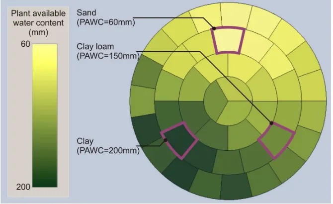
[image:5.595.131.466.503.708.2]In a simulation, cotton was sown on a 400 m diameter centre pivot-irrigated field on 4 October and was irrigated until 14 March of the following year. Nitrogen application was 250 kg/ha at the start of the season and a cell size of 2900 m² was specified (i.e. cells were approximately 50 m wide and 60 m long). The soil moisture deficit at the start of the season was the plant available water content and the irrigation machine capacity was 15 mm/day. The spatially varied soil properties (i.e. plant available water content) produced the underlying variability for the simulations presented in this case study (Figure 1).
For ILC, the irrigations were initiated after 40 mm of crop water use and the irrigation volumes were varied to target a soil moisture deficit of 80 mm after each irrigation. The feedback soil moisture data was obtained from the OZCOT model one day after each irrigation event. For MPC, the irrigations occurred daily and the final crop yield predicted by the model was maximised. The daily weather profile used was obtained from the Australian Bureau of Meteorology SILO data (QNRM 2009) for 2004/2005. Simulations of the two control strategies were conducted using different levels of input data (i.e. one, three, ten and all cells in the field). For ILC, soil moisture data was available for these cells, whilst for MPC, soil moisture data and plant information (i.e. leaf area index, square count, boll count) were available for these cells. Ten replicates of each spatial resolution have been simulated with the cells selected randomly across the field.
Results
Iterative learning control (ILC) strategy performance
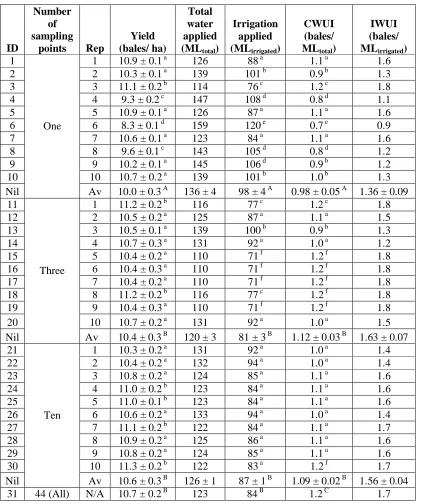
The simulated yield and water use efficiency (Table 1) was generally consistently high using ILC and with all three scales of spatial data input. The highest average yield was obtained using input from three, ten or all data points in the field. ILC was sensitive to the location of the point used with a single data point input (i.e. as the yields of simulations 4, 6 and 8 are significantly lower than the other simulations). However, with three or ten data input points ILC was less sensitive to the unmeasured spatial variability of the soil properties as a high crop yield was generally maintained. This is because the soil moisture in the cells without measured data was estimated using the spatial interpolation procedure. Any error between the estimated soil moisture status and actual soil moisture status in the unmeasured cells did not generally affect the crop yield. This error would have caused the ILC algorithm to maintain a different soil moisture deficit to that specified (80 mm). However, this error did not cause the crop to be water stressed. The standard error (i.e. spatial variability) of the yield was also low for all simulations. As the number of sampling points in the field increased the following general observations were made:
• the average yield increased;
• the irrigation volume applied decreased;
• the crop water use efficiency increased significantly between one and there points but not between three and ten or all points; this indicates that using three data inputs is as useful as all inputs for ILC; and
• the consistency of the average yield and irrigation applied across the field improved. This indicates that the crop yield and irrigation applied are less sensitive to the location of the input data points in the field as the number of data points increases.
points. The table shows the average and standard error of the simulated outputs for ten replications of simulations; and within columns the use of matching superscripts (a, b, … l) indicates no significant difference (at the 95% significance level) within the replications. The table also shows the average and standard error of each set of simulations with a different number of sampling points (in rows with ‘Av’) and the simulation using all data points; and within the columns the use of matching superscripts (A, B, ... F) indicates significant difference (at the 95% significance level) between the sets of replications and the simulation with input from all data points.
ID
Number of sampling
points Rep
Yield (bales/ ha)
Total water applied (MLtotal)
Irrigation applied (MLirrigated)
CWUI (bales/ MLtotal)
IWUI (bales/ MLirrigated)
1 1 10.9 ± 0.1 a 126 88 a 1.1 a 1.6
2 2 10.3 ± 0.1 a 139 101 b 0.9 b 1.3
3 3 11.1 ± 0.2 b 114 76 c 1.2 c 1.8
4 4 9.3 ± 0.2 c 147 108 d 0.8 d 1.1
5 5 10.9 ± 0.1 a 126 87 a 1.1 a 1.6
6 6 8.3 ± 0.1 d 159 120 e 0.7 e 0.9
7 7 10.6 ± 0.1 a 123 84 a 1.1 a 1.6
8 8 9.6 ± 0.1 c 143 105 d 0.8 d 1.2
9 9 10.2 ± 0.1 a 145 106 d 0.9 b 1.2
10 10 10.7 ± 0.2 a 139 101 b 1.0 b 1.3
Nil
One
Av 10.0 ± 0.3 A 136 ± 4 98 ± 4 A 0.98 ± 0.05 A 1.36 ± 0.09
11 1 11.2 ± 0.2 b 116 77 c 1.2 c 1.8
12 2 10.5 ± 0.2 a 125 87 a 1.1 a 1.5
13 3 10.5 ± 0.1 a 139 100 b 0.9 b 1.3
14 4 10.7 ± 0.3 a 131 92 a 1.0 a 1.2
15 5 10.4 ± 0.2 a 110 71 f 1.2 f 1.8
16 6 10.4 ± 0.3 a 110 71 f 1.2 f 1.8
17 7 10.4 ± 0.2 a 110 71 f 1.2 f 1.8
18 8 11.2 ± 0.2 b 116 77 c 1.2 f 1.8
19 9 10.4 ± 0.3 a 110 71 f 1.2 f 1.8
20 10 10.7 ± 0.2 a 131 92 a 1.0 a 1.5
Nil
Three
Av 10.4 ± 0.3 B 120 ± 3 81 ± 3 B 1.12 ± 0.03 B 1.63 ± 0.07
21 1 10.3 ± 0.2 a 131 92 a 1.0 a 1.4
22 2 10.4 ± 0.2 a 132 94 a 1.0 a 1.4
23 3 10.8 ± 0.2 a 124 85 a 1.1 a 1.6
24 4 11.0 ± 0.2 b 123 84 a 1.1 a 1.6
25 5 11.0 ± 0.1 b 123 84 a 1.1 a 1.6
26 6 10.6 ± 0.2 a 133 94 a 1.0 a 1.4
27 7 11.1 ± 0.2 b 122 84 a 1.1 a 1.7
28 8 10.9 ± 0.2 a 125 86 a 1.1 a 1.6
29 9 10.8 ± 0.2 a 124 85 a 1.1 a 1.6
30 10 11.3 ± 0.2 b 122 83 a 1.2 f 1.7
Nil
Ten
Model predictive control (MPC) strategy performance
The MPC controller was simulated with the input of data from the same random data points in the field as the ILC controller (Table 2). As the spatial scale of input data reduced (i.e. the number of input data points increased), the following general observations were made:
• the crop and irrigation water use efficiencies increased; • the irrigation volume application reduced; and
• as per ILC, the consistency of the average yield and irrigation applied across the field improved.
The location of the data points in the field affected the yield and water use efficiency. This effect was the greatest in the simulations of one data input in the field. For example, the use of one point of data input led to yields and water use efficiencies higher than several simulations using three or ten data points (e.g. simulation 38), while also leading to the lowest yield and water use efficiency of all the simulations (i.e. simulation 35). Hence, the location of the point in the field limits the performance of MPC.
There was no significant difference between the average yield or water use of the simulations using data from three and ten points in the field. However, the yield and water use efficiency of the simulations using data from ten points was greater than those of the simulations using data from one or three points. This indicates that the input of data from one or three points in the field does not provide sufficient spatial information to accurately calibrate the crop model. The greatest average yield and water use efficiency was provided with input from all data points in the field.
The standard error of the yield for the simulations with ten data input points was higher those those with one or three data iput points. This is because the number of cells with known properties – and hence accurately optimised yield – increased, leading to a more accurate spatial interpolation of the cell properties. The cells with estimated soil and crop properties have lower yields than the cells that have measured properties because of the errors in the estimated properties used to optimise the yield.
Comparison of iterative learning and model predictive control strategies
The ILC controller produced higher yields and water use efficiencies than the MPC controller for all scales of spatial data input; hence, in low data situations ILC outperformed MPC. When a complete data set was available for each cell in the field, the simulated yield and water use efficiency was higher for the MPC controller than the ILC controller.
points. The table shows the average and standard error of the simulated outputs for ten replications of simulations; and within columns the use of matching superscripts (a, b, … l) indicates no significant difference (at the 95% significance level) within the replications. The table also shows the average and standard error of each set of simulations with a different number of sampling points (in rows with ‘Av’) and the simulation using all data points; and within the columns the use of matching superscripts (A, B, ... F) indicates significant difference (at the 95% significance level) between the sets of replications and the simulation with input from all data points.
ID
Number of sampling
points Rep
Yield (bales/ ha)
Total water applied
(ML)
Irrigation applied
(ML)
CWUI (bales/ MLtotal)
IWUI (bales/ MLirrigated)
32 1 4.1 ± 0.1 e 119 81 g 0.4 g 0.6
33 2 3.1 ± 0.2 f 105 67 f 0.4 g 0.6
34 3 2.5 ± 0.2 g 97 60 h 0.3 h 0.5
35 4 2.0 ± 0.2 h 93 56 h 0.3 i 0.5
36 5 5.1 ± 0.1 i 141 103 b 0.5 g 0.6
37 6 5.2 ± 0.1 i 134 96 a 0.5 g 0.7
38 7 5.8 ± 0.2 j 125 87 a 0.6 j 0.8
39 8 4.4 ± 0.1 k 124 86 a 0.4 g 0.6
40 9 5.7 ± 0.3 j 128 89 a 0.6 j 0.8
41 10 2.3 ± 0.2 g 89 52 i 0.3 i 0.6
Nil
One
Av 3.9 ± 0.3 C 116 ± 6 78 ± 6 C 0.42 ± 0.03 D 0.63 ± 0.03
42 1 3.5 ± 0.1 l 101 62 f 0.4 g 0.7
43 2 3.4 ± 0.2 l 110 72 f 0.4 g 0.6
44 3 4.4 ± 0.1 k 117 78 c 0.5 g 0.7
45 4 3.8 ± 0.2 e 117 79 c 0.4 g 0.6
46 5 4.1 ± 0.1 e 117 78 c 0.4 g 0.7
47 6 4.3 ± 0.2 k 110 71 f 0.5 g 0.8
48 7 3.9 ± 0.2 e 109 70 f 0.5 g 0.7
49 8 3.9 ± 0.1 e 115 76 c 0.4 g 0.6
50 9 3.4 ± 0.2 l 110 72 f 0.4 g 0.6
51 10 3.4 ± 0.2 l 103 64 f 0.4 g 0.7
Nil
Three
Av 3.7 ± 0.2 C 111 ± 2 72 ± 2 C 0.43 ± 0.01 D 0.67 ± 0.02
52 1 6.2 ± 0.6 j 117 78 c 0.7 e 1.0
53 2 5.2 ± 0.6 i 110 71 f 0.6 j 0.9
54 3 5.7 ± 0.5 j 105 67 f 0.7 e 1.1
55 4 6.1 ± 0.5 j 116 77 c 0.7 e 1.0
56 5 5.8 ± 0.6 j 105 67f 0.7 e 1.1
57 6 5.2 ± 0.6 i 101 63 f 0.6 j 1.0
58 7 5.4 ± 0.6 i 111 73 f 0.6 j 0.9
59 8 5.0 ± 0.6 i 109 71 f 0.6 j 0.9
60 9 4.9 ± 0.6 i 96 58 h 0.6 j 1.1
61 10 5.9 ± 0.6 j 115 76 c 0.6 j 1.0
Nil
Ten
CONCLUSION
Iterative learning and model predictive control strategies were implemented and simulated for irrigation optimisation of a cotton crop. The strategies were compared for robustness to sparse data input. The iterative learning controller outperformed the model predictive controller in low data situations, whilst the model predictive controller produced higher yield and water use efficiency than the iterative learning controller with a full data set.
Acknowledgements
The authors are grateful to the Australian Research Council and the Cotton Research and Development Corporation for funding a postgraduate studentship for the senior author.
REFERENCES
Ahn, H.-S., K. L. Moore and Y. Chen. 2007. Iterative learning control: robustness and monotonic convergence for interval systems, Communications and Control
Engineering, Springer, London.
Evans, R. G. 2006. Irrigation technologies. Sidney, Montana. Available at:
http://www.sidney.ars.usda.gov/Site_Publisher_Site/pdfs/personnel/Irrigation%20Tech nologies%20Comparisons.pdf. Accessed 19 June 2007.
Kwon, W. and S. Han. 2005. Receding horizon control: model predictive control for state models, Advanced textbooks in control and signal processing, Springer-Verlag,
London.
McCarthy, A. C., N. H. Hancock and S. R. Raine. 2010. VARIwise: a general-purpose adaptive control simulation framework for spatially and temporally varied irrigation at sub-field scale. Computers and Electronics in Agriculture. 70(1): 117-128.
Moore, K. L. and Y. Chen. 2006. Iterative learning control approach to a diffusion control problem in an irrigation application. IEEE International Conference on Mechatronics and Automation. LuoYang, China, pp. 1329-1334.
Park, Y., J. Shamma, J. and T. Harmon. 2009. A receding horizontal control algorithm for adaptive management of soil moisture and chemical levels during irrigation,
Environmental Modelling & Software. 24(9): 1112-1121.
QNRM 2009. Queensland Natural Resources and Mines enhanced meteorological datasets. Australia. Available at: http://www.longpaddock.qld.gov.au/silo/. Accessed 10 October 2009.
Smith, R. J., S. R. Raine, A. C. McCarthy and N. H. Hancock. 2009. Managing spatial and temporal variability in irrigated agriculture through adaptive control. Australian
Journal of Multi-disciplinary Engineering. 7(1): 79-90.
Warwick, K. 1993. Adaptive control. In: S. G. Tzafestas, ed., Applied control, Electrical and Computer Engineering, Marcel Dukker Inc. New York. Ch. 9. pp. 253-271. Wells, A and A. Hearn. 1992. OZCOT: a cotton crop simulation model for management.