Near-Field
Thesis by Regina Sullivan
In Partial Fulfillment of the Requirements for the Degree of
Doctor of Philosophy
California Institute of Technology Pasadena, California
2010
c
2010
Acknowledgements
I would like to take the opportunity to thank the following individuals:
• Jan, Pat, and Owen Sullivan, thesine qua nonof my life and academic career. (Thanks for always being there to answer the phone at 3 am!)
• Lee Johnson, my mentor for the past 7 and 1/2 years and my PhD advisor at JPL, for teaching me how to be a good researcher, for always showing great patience with my non-so-well-thought-out questions, and also for helping me learn many valuable life skills (motorcycle riding, guitar playing, etc.).
• Joseph Shepherd, my PhD advisor, for his academic, research, and career advice, and for giving me a crash course in numerical methods for solving differential equations.
• David Conroy, my officemate, for providing good advice, good music, and good con-versation.
• Michelle Scharfe, for her invaluable assistance with modeling, for writing some code for me, and for being really nice to me the first summer I interned at JPL.
• Yiangos Mikellides, for helping me develop my sheath model, and for figuring out a way to implement those pesky boundary conditions.
• Rich Hofer, for providing me with the HPHall code and answering my many questions about it.
• Ray Swindlehurst and Al Owens, for helping me in the machine shop.
• Paul Bellan and Dale Pullin, for taking time out of their undoubtedly busy schedules to serve on both my candidacy and thesis defense committees.
I would also like to thank the following programs/institutions for funding my research:
• National Science Foundation Graduate Research Fellowship Program
• Air Force Research Laboratory
Abstract
A study of the physics underlying high velocity ion trajectories within the near-field region of a Hall thruster plume is presented. In this context, “high velocity” ions are ions that have been accelerated through the full potential drop of the thruster (sometimes referred to as “primary energy” or “primary beam energy” ions). Results from an experimental survey of an SPT-70 thruster plume are shown, along with simulated data from a Hall thruster code and from a plasma sheath model. Two main features are examined: the central jet along the Hall thruster centerline, and the population of high velocity ions at high angles.
In the experimental portion of the investigation, three diagnostic instruments were employed: (1) a Faraday probe for measuring ion current density, (2) an ExB velocity filter for mapping ions with the primary beam energy, and (3) a Retarding Potential Analyzer (RPA) for determining ion energy distributions. In the numerical portion, two codes were employed: (1) a hybrid-PIC Hall thruster code known as HPHall, and (2) a model of the plasma sheath near the exit plane of the thruster, which was developed by the author.
Contents
Acknowledgements v
Abstract vii
Nomenclature/Symbols xxii
1 Introduction 1
1.1 Hall Thruster Overview . . . 1
1.2 Previous Research . . . 4
1.3 Motivation . . . 4
1.4 Problem Statement and Approach . . . 5
2 Experimental Method 7 2.1 SPT-70 Thruster . . . 7
2.2 Vacuum Facility . . . 8
2.3 Diagnostic Instruments - Faraday Probe . . . 10
2.3.1 Instrument Overview . . . 10
2.3.2 Instrument Design and Data Acquistion System . . . 12
2.3.3 Uncertainty Analysis . . . 12
2.4 Diagnostic Instruments - ExB Velocity Filter . . . 13
2.4.1 Instrument Overview . . . 13
2.4.2 Instrument Design and Data Acquisition System . . . 15
2.4.3 Uncertainty Analysis . . . 21
2.5 Diagnostic Instruments - Retarding Potential Analyzer . . . 24
2.5.2 Instrument Design and Data Acquisition System . . . 25
2.5.3 Uncertainty Analysis . . . 28
2.6 Summary of Scans . . . 30
3 Simulation Approach - HPHall 34 3.1 Hybrid-PIC Model Overview . . . 34
3.1.1 Electron Sub-model . . . 35
3.1.2 Heavy Particle Sub-model . . . 38
3.1.3 Wall Interactions . . . 40
3.2 HPHall at the Jet Propulsion Laboratory . . . 41
3.3 Application to the Ion Trajectory Problem . . . 43
3.3.1 HPHall Solution Domain . . . 43
3.3.2 Magnetic Field and Electron Mobility Analysis . . . 43
3.3.3 Ion Tracking and Energy Distributions . . . 49
3.3.4 Oscillation Analysis . . . 50
4 Simulation Approach - Corner Sheath Model 52 4.1 Corner Sheath Model - Motivation . . . 52
4.2 Sheath Equations . . . 54
4.3 Boundary Conditions . . . 55
4.4 Numerical Method . . . 57
4.5 Model Verification . . . 60
4.6 “Quasi”-2D Application . . . 60
5 Experimental Results and Discussion 66 5.1 Results and Discussion - ExB Filter and Faraday Probe . . . 66
5.1.1 Transverse Scans . . . 68
5.1.1.1 200 W Results . . . 74
5.1.1.2 650 W Results . . . 80
5.1.2 Axial Scans . . . 80
5.2 Uncertainty in the ExB Data . . . 85
5.3 RPA Analysis . . . 87
5.5 Sputter Yield Analysis . . . 96
6 HPHall Results and Discussion 102 6.1 HPHall Run Conditions . . . 103
6.2 Time Averaged Results from HPHall . . . 103
6.2.1 650 W Results . . . 103
6.2.2 200 W Results . . . 116
6.2.3 Asymmetry of Ion Density Plots . . . 128
6.2.4 Comparison of averaged data to existing studies . . . 130
6.3 Faraday Probe and ExB Plots from HPHall . . . 132
6.3.1 Faraday Probe Results . . . 132
6.3.2 ExB Probe Results . . . 137
6.4 RPA Results from HPHall . . . 147
6.4.1 650 W results . . . 147
6.4.2 200 W results . . . 152
6.5 Repeatability of the Simulated Results . . . 156
6.6 Effect of Oscillations . . . 159
7 Corner Sheath Model Results and Discussion 165 7.1 Boundary Conditions . . . 165
7.2 Potential Profile . . . 166
7.3 Ion Trajectories Through the Sheath . . . 172
8 Comparison of Experimental and Simulated Results 182 8.1 Formation of the Central Jet . . . 183
8.2 Angles of Ion Trajectories within the Near Field Plume . . . 184
8.3 High Velocity High Angle Ions . . . 186
9 Conclusions and Recommendations 192 9.1 Conclusions . . . 192
9.2 Recommendations for Future Work . . . 193
B Additional Experimental RPA Data 211
B.1 Raw RPA Data . . . 211 B.2 Differentiated RPA Data (not normalized) . . . 218 B.3 Sputter Yield Data . . . 225
C Additional HPHall Oscillation Results 227
D Additional HPHall Simulated ExB Probe Results 235
List of Figures
1.1 Hall thruster cross section . . . 3
1.2 SPT-70 plume . . . 3
2.1 SPT-70 thruster . . . 9
2.2 SPT-70 erosion . . . 9
2.3 Big Green vacuum chamber . . . 10
2.4 Translation stage schematic . . . 11
2.5 Faraday probe schematic . . . 11
2.6 Faraday probe used in the experiment . . . 13
2.7 Faraday probe data acquisition system . . . 14
2.8 ExB schematic . . . 15
2.9 ExB sample trace . . . 16
2.10 Colutron Model 300 velocity filter . . . 16
2.11 ExB probe used in experiment . . . 17
2.12 ExB alignment . . . 18
2.13 ExB potential distribution . . . 19
2.14 ExB magnetic field . . . 19
2.15 ExB data acquisition system . . . 20
2.16 ExB resolution . . . 22
2.17 RPA schematic . . . 24
2.18 RPA sample trace . . . 25
2.19 RPA photo . . . 26
2.20 RPA data acquisition system . . . 27
2.21 Example result from Simion . . . 29
2.23 RPA scans . . . 32
3.1 HPHall program flow . . . 36
3.2 SPT-70 solution domain . . . 37
3.3 Transformation from r-z to ξ−η plane . . . 38
3.4 Shape of plasma sheath at wall . . . 40
3.5 Possible potential distributions . . . 44
3.6 Measured SPT-70 magnetic field, 200 W case . . . 45
3.7 Measured SPT-70 magnetic field, 650 W case . . . 46
3.8 Simulated Faraday probe trajectory projection . . . 50
3.9 Simulated RPA trajectory projection . . . 51
4.1 Bending of ion trajectories due to the sheath . . . 53
4.2 Corner sheath model program flow . . . 58
4.3 Comparison of 1D to 2D model, example 1 . . . 61
4.4 Comparison of 1D to 2D model, example 2 . . . 62
4.5 Comparison of 1D to 2D model, example 3 . . . 63
4.6 Corner sheath model solution domain . . . 64
4.7 Applying the 2D solver in a quasi-2D fashion . . . 65
5.1 Transverse scans taken with the ExB filter . . . 68
5.2 Compiled ExB results, 200 W . . . 69
5.3 Compiled ExB results, 650 W . . . 70
5.4 Compiled FP results, 200 W . . . 71
5.5 Compiled FP results, 650 W . . . 72
5.6 ExB results, 200 W case, at 50 mm . . . 76
5.7 ExB results, 200 W case, at 100 mm . . . 77
5.8 ExB results, 200 W case, at 150 mm . . . 78
5.9 Faraday probe results, 200 W case . . . 79
5.10 ExB results, 650 W case, at 50 mm . . . 81
5.11 ExB results, 650 W case, at 100 mm . . . 82
5.12 ExB results, 650 W case, at 150 mm . . . 83
5.14 ExB axial results, 200 W . . . 86
5.15 ExB axial results, 650 W . . . 86
5.16 Differentiated RPA data at 200 W, 0 to 40◦ . . . 90
5.17 Differentiated RPA data at 200 W, 45 to 65◦ . . . 91
5.18 Differentiated RPA data at 200 W, 70 to 90◦ . . . 92
5.19 Differentiated RPA data at 650 W, 0 to 40◦ . . . 93
5.20 Differentiated RPA data at 650 W, 45 to 65◦ . . . 94
5.21 Differentiated RPA data at 650 W, 70 to 90◦ . . . 95
5.22 Example of sputter yield calculation. . . 98
5.23 Sputter yield estimate for C, 200 W . . . 99
5.24 Sputter yield estimate for Si, 200 W . . . 99
5.25 Sputter yield estimate for Al, 200 W . . . 99
5.26 Sputter yield estimate for Ti, 200 W . . . 100
5.27 Sputter yield estimate for C, 650 W . . . 100
5.28 Sputter yield estimate for Si, 650 W . . . 100
5.29 Sputter yield estimate for Al, 650 W . . . 101
5.30 Sputter yield estimate for Ti, 650 W . . . 101
6.1 Averaged plasma potential from HPHall, 650 W upstream run . . . 106
6.2 Averaged axial electric field from HPHall, 650 W upstream run . . . 107
6.3 Averaged radial electric field from HPHall, 650 W upstream run . . . 108
6.4 Averaged electron temperature from HPHall, 650 W upstream run . . . 109
6.5 Averaged ion density from HPHall, 650 W upstream run . . . 110
6.6 Averaged plasma potential from HPHall, 650 W downstream run . . . 111
6.7 Averaged axial electric field from HPHall, 650 W downstream run . . . 112
6.8 Averaged radial electric field from HPHall, 650 W downstream run . . . 113
6.9 Averaged electron temperature from HPHall, 650 W downstream run . . . . 114
6.10 Averaged ion density from HPHall, 650 W downstream run . . . 115
6.11 Averaged plasma potential from HPHall, 200 W upstream run . . . 118
6.12 Averaged axial electric field from HPHall, 200 W upstream run . . . 119
6.13 Averaged radial electric field from HPHall, 200 W upstream run . . . 120
6.15 Averaged ion density from HPHall, 200 W upstream run . . . 122
6.16 Averaged plasma potential from HPHall, 200 W downstream run . . . 123
6.17 Averaged axial electric field from HPHall, 200 W downstream run . . . 124
6.18 Averaged radial electric field from HPHall, 200 W downstream run . . . 125
6.19 Averaged electron temperature from HPHall, 200 W downstream run . . . . 126
6.20 Averaged ion density from HPHall, 200 W downstream run . . . 127
6.21 Plasma potential from HPHall at different axial locations, 650 W upstream run 129 6.22 Plasma potential from HPHall at different axial locations, 650 W downstream run . . . 129
6.23 Plasma potential from HPHall at different axial locations, 200 W upstream run 129 6.24 Plasma potential from HPHall at different axial locations, 200 W downstream run . . . 130
6.25 Faraday probe traces created from HPHall data, 650 W runs . . . 134
6.26 Faraday probe traces created from HPHall data, 200 W runs . . . 135
6.27 Faraday probe traces created from HPHall data, 25mm, all runs . . . 136
6.28 ExB probe traces created from HPHall data at 50 mm, 650 W runs . . . 139
6.29 ExB probe traces created from HPHall data at 50 mm, 650 W runs, ion current140 6.30 ExB probe traces created from HPHall data at 100 mm, 650 W runs . . . . 141
6.31 ExB probe traces created from HPHall data at 150 mm, 650 W runs . . . . 142
6.32 ExB probe traces created from HPHall data at 50 mm, 200 W runs . . . 144
6.33 ExB probe traces created from HPHall data at 100 mm, 200 W runs . . . . 145
6.34 ExB probe traces created from HPHall data at 150 mm, 200 W runs . . . . 146
6.35 RPA traces created from HPHall data, 650 W runs, 0 to 40 deg . . . 149
6.36 RPA traces created from HPHall data, 650 W runs, 45 to 65 deg . . . 150
6.37 RPA traces created from HPHall data, 650 W runs, 70 to 80 deg . . . 151
6.38 RPA traces created from HPHall data, 200 W runs, 0 to 40 deg . . . 153
6.39 RPA traces created from HPHall data, 200 W runs, 45 to 65 deg . . . 154
6.40 RPA traces created from HPHall data, 200 W runs, 70 to 80 deg . . . 155
6.41 Bound on the simulated RPA data . . . 157
6.42 Oscillation tracking in HPHall, 650 W upstream run . . . 162
7.1 Boundary conditions for the corner sheath model, 650 W upstream run . . . 167
7.2 Boundary conditions for the corner sheath model, 650 W downstream run . . 168
7.3 Boundary conditions for the corner sheath model, 200 W upstream run . . . 169
7.4 Boundary conditions for the corner sheath model, 200 W downstream run . . 170
7.5 Plasma potential from the corner sheath model, 650 W upstream run . . . . 170
7.6 Plasma potential from the corner sheath model, 650 W downstream run . . . 171
7.7 Plasma potential from the corner sheath model, 200 W upstream run . . . . 171
7.8 Plasma potential from the corner sheath model, 200 W downstream run . . . 171
7.9 Trajectories from the corner sheath model, 650 W upstream run, U0 = 2.5 . 174 7.10 Trajectories from the corner sheath model, 650 W upstream run, U0 = 5.0 . 175 7.11 Trajectories from the corner sheath model, 650 W downstream run, U0 = 2.5 176 7.12 Trajectories from the corner sheath model, 650 W downstream run, U0 = 5.0 177 7.13 Trajectories from the corner sheath model, 200 W upstream run, U0 = 2.5 . 178 7.14 Trajectories from the corner sheath model, 200 W upstream run, U0 = 5.0 . 179 7.15 Trajectories from the corner sheath model, 200 W downstream run, U0 = 2.5 180 7.16 Trajectories from the corner sheath model, 200 W downstream run, U0 = 5.0 181 8.1 Potential profiles from HPHall versus theoretical potential profile . . . 189
A.1 ExB results, 200 W case, at 0◦ . . . 198
A.2 ExB results, 200 W case, at 10◦ . . . 199
A.3 ExB results, 200 W case, at 20◦ . . . 200
A.4 ExB results, 200 W case, at 30◦ . . . 201
A.5 ExB results, 200 W case, at 40◦ . . . 202
A.6 ExB results, 200 W case, at 50◦ . . . 203
A.7 ExB results, 200 W case, at 60◦ . . . 204
A.8 ExB results, 650 W case, at 0◦ . . . 205
A.9 ExB results, 650 W case, at 10◦ . . . 206
A.10 ExB results, 650 W case, at 20◦ . . . 207
A.11 ExB results, 650 W case, at 30◦ . . . 208
A.12 ExB results, 650 W case, at 40◦ . . . 209
B.2 RPA raw data, 200W, from 45 to 65◦ . . . 213
B.3 RPA raw data, 200W, from 70 to 90◦ . . . 214
B.4 RPA raw data, 650W, from 0 to 40◦ . . . 215
B.5 RPA raw data, 650W, from 45 to 65◦ . . . 216
B.6 RPA raw data, 650W, from 70 to 90◦ . . . 217
B.7 RPA differentiated data, 200W, from 0 to 40◦ . . . 219
B.8 RPA differentiated data, 200W, from 45 to 65◦ . . . 220
B.9 RPA differentiated data, 200W, from 70 to 90 degrees . . . 221
B.10 RPA differentiated data, 650W, from 0 to 40◦ . . . 222
B.11 RPA differentiated data, 650W, from 45 to 65◦ . . . 223
B.12 RPA differentiated data, 650W, from 70 to 90◦ . . . 224
B.13 Sputter yield, Carbon . . . 225
B.14 Sputter yield, Silicon . . . 225
B.15 Sputter yield, Aluminum . . . 226
B.16 Sputter yield, Titanium . . . 226
C.1 Oscillation tracking in HPHall, 650 W downstream run . . . 228
C.2 Frequency spectrum, 650 W downstream run . . . 229
C.3 Oscillation tracking in HPHall, 200 W upstream run . . . 230
C.4 Frequency spectrum, 200 W upstream run . . . 231
C.5 Oscillation tracking in HPHall, 200 W downstream run . . . 232
C.6 Frequency spectrum, 200 W downstream run . . . 233
D.1 ExB probe traces created from HPHall data at 50 mm, 650 W runs, ion current236 D.2 ExB probe traces created from HPHall data at 100 mm, 650 W runs, ion current237 D.3 ExB probe traces created from HPHall data at 150 mm, 650 W runs, ion current238 D.4 ExB probe traces created from HPHall data at 50 mm, 200 W runs, ion current239 D.5 ExB probe traces created from HPHall data at 100 mm, 200 W runs, ion current240 D.6 ExB probe traces created from HPHall data at 150 mm, 200 W runs, ion current241
List of Tables
2.1 Faraday probe dimensions . . . 12
2.2 RPA uncertainty due to ion optics . . . 30
2.3 Summary of Faraday probe scans . . . 32
2.4 ExB scan summary . . . 33
2.5 RPA scan summary . . . 33
3.1 Cathode and anode parameters for HPHall . . . 43
3.2 Description of the four cases modeled in HPHall . . . 48
3.3 Performance parameters of the cases modeled in HPHall . . . 48
6.1 Description of the four runs modeled in HPHall . . . 103
6.2 Averaged data from previous HPHall studies . . . 131
6.3 Averaged data from current HPHall study . . . 131
6.4 Maximum error in the simulated Faraday probe data . . . 156
6.5 Maximum error in the simulated ExB data . . . 158
6.6 Maximum error in the simulated RPA data . . . 158
6.7 Summary of oscillation data from HPHall . . . 161
7.1 Trajectories through sheath, U0 = 2.5, 650 W upstream run . . . 174
7.2 Trajectories through sheath, U0 = 5.0, 650 W upstream run . . . 175
7.3 Trajectories through sheath, U0 = 2.5, 650 W downstream run . . . 176
7.4 Trajectories through sheath, U0 = 5.0, 650 W downstream run . . . 177
7.5 Trajectories through sheath, U0 = 2.5, 200 W upstream run . . . 178
7.6 Trajectories through sheath, U0 = 5.0, 200 W upstream run . . . 179
7.7 Trajectories through sheath, U0 = 2.5, 200 W downstream run . . . 180
E.1 Trajectories through sheath, U0 = 7.5, 650 W upstream run . . . 243
E.2 Trajectories through sheath, U0 = 10.0, 650 W upstream run . . . 244
E.3 Trajectories through sheath, U0 = 7.5, 650 W downstream run . . . 245
E.4 Trajectories through sheath, U0 = 10.0, 650 W downstream run . . . 246
E.5 Trajectories through sheath, U0 = 7.5, 200 W upstream run . . . 247
E.6 Trajectories through sheath, U0 = 10.0, 200 W upstream run . . . 248
E.7 Trajectories through sheath, U0 = 7.5, 200 W downstream run . . . 249
Nomenclature/Symbols
µ0 = permeability of free space = 1.26x10⁻⁶ m kg s−2 A−2 0 = permittivity of free space = 8.85x10⁻¹²m−3 kg−1 s4 A2 k= Boltzmann constant = 1.38x10⁻²³ m2 kg s−2 K−1 e= elementary charge = 1.60x10⁻¹⁹ C
σ = magnetic potential function λ= magnetic stream function ni = ion density
ne = electron density nn = neutral density Te = electron temperature ui = ion velocity
φ= plasma potential
µe⊥ cross-field electron mobility
Ωe = electron Hall parameter ωce = electron cyclotron frequency
νe = total effective electron collision frequency νen = electron-neutral collision frequency νei = electron-ion collision frequency νw = electron-wall collision frequency νb = anomalous collision frequency λD = debye length
us = ion acoustic speed
˜
∇= non-dimensional partial derivative
˜
n= non-dimensional ion density ~
χ = non-dimensional plasma potential
˜
E = non-dimensional electric field
Chapter 1
Introduction
1.1
Hall Thruster Overview
As with other types of electric propulsion (EP) devices, Hall thrusters offer the benefits of high efficiencies and long lifetimes. Such advantages make these thrusters well-suited for a variety of in-space applications, especially those requiring adjustments to spacecraft velocity over long periods of time. For example, satellite station-keeping and planetary exploration are some of the more prominent applications of EP technology over its nearly 50-year development history. Hall thrusters, notably, were used on Russian satellites as early as 1974 [1]. Recently, Hall thrusters have been employed on a variety of missions. Space Systems/Loral, for example, has used the Russian manufactured SPT-100 thruster on a number of their commercial satellites [2]. Additionally, the TacSat-2 mission conducted by the U.S. Air Force was the first use of a U. S. developed Hall thruster on a satellite [3]. Hall thrusters also provided the propulsion for the ESA SMART-1 lunar orbiter [4].
Hall thrusters, and their close counterparts, ion thrusters, are able to achieve high specific impulses (and thus low propellant masses) due to the high exhaust velocities that they produce. In both of these types of thrusters, electrical energy is converted to kinetic energy through the acceleration of an ionized gas. However, in an ion thruster this accelera-tion occurs between two grids, while in a Hall thruster the acceleraaccelera-tion region is not defined by a physical barrier. For this reason, the behavior of the resulting ion exhaust is less easily predicted in the case of the Hall thruster.
propellant gas (usually Xenon) is introduced at the upstream end of the insulated cylindrical channel. At the same time, electrons are generated at the cathode. Due to their thermal motion, the electrons distribute themselves across the face of the thruster, while the presence of the positive anode draws them into the channel.
As these electrons migrate upstream, they encounter the radial magnetic field and begin to undergo orbits about these field lines, essentially becoming trapped in the region of high magnetic field. This decrease in electron mobility causes a primarily axial electric field to develop along the length of the channel. Propellant atoms, moving from upstream, undergo collisions with the trapped electrons. If the energy of a collision is sufficient, ionization will occur. The ions generated will then be accelerated out of the channel by the axial electric field, producing an annular ion beam [5].
In a conventional chemical rocket nozzle, the thrust force is transmitted to the thruster body through direct contact with the propellant. However, in a Hall thruster, the argument has been made that the thrust force is transmitted through the magnetic field [5]. This occurs because of the ”partially magnetized” nature of the plasma, in which the electrons are trapped on magnetic field lines while the ions are not. As the ions are accelerated downstream by the electric field, they tend to want to drag the electrons with them. However, the Lorentz force (Fmag=q(~v×B~)) keeps the electrons from being pulled along with the ions. The magnetic field thus exerts a force on the electrons that is in the upstream direction. The equal and opposite force between the electrons and the magnetic field, in the downstream direction, is the thrust force.
e
-Xe
+, Xe
++, etc.
Xe
+
-B
E
CL
magnetic coil
cath od
e
anode
magnetic coil insulator
e
-Xe
+, Xe
++, etc.
Xe
+
-B
E
CL
magnetic coil
cath od
e
anode
[image:27.595.156.504.69.361.2]magnetic coil insulator
Figure 1.1: Hall thruster cross section. Note that the full thruster is cylindrically symmetric about the centerline.
[image:27.595.148.482.429.685.2]1.2
Previous Research
In terms of experimental research, some studies have been conducted that focus on ion tra-jectories within the near-field region of the Hall thruster plume. For example, Laser-Induced-Fluorescence (LIF) techniques have been used by the researchers at the Air Force Research Laboratory (AFRL) to investigate ion velocities near the exit plane of a Hall thruster [6– 9]. However, most experimental studies of the Hall thruster near-field region have looked at plasma parameters such as potential, ion density, and electron temperature [10–12], because these parameters can be measured using fast moving probes that cause minimal disturbance to the thruster plasma. For the most part, experimental investigations of ion energy and trajectory angles have used diagnostics that were located far from the thruster exit plane [12, 13].
Simulations of Hall thrusters have focused primarily on two areas: (1) the internal physics inside the thruster channel, and (2) the ”far-field” region that is several thruster diameters downstream of the exit plane. The method that has been most widely used to model the thruster channel is the ”hybrid-PIC” approach which treats electrons as a fluid and ions as particles-in-cell. Most research groups involved in the modeling of Hall thrusters have developed codes which use this method [14–18]. In these codes, the simulation domain usually consists of the Hall thruster channel plus a small region downstream of the exit plane within the near-field. In regards to the far-field codes, these simulations typically use DSMC methods to model collisions within the thruster plume [19, 20]. While these codes do a suitable job of modeling plume expansion, they require an input boundary condition to work. If the input condition that is applied poorly reflects the actual situation, then the far-field codes will not produce accurate results.
1.3
Motivation
result, the simulation region of most hybrid-PIC codes only extends out a few centimeters downstream of the exit plane, and thus cannot fully capture near-field phenomena. As far as the far-field simulations are concerned, these codes were created with the goal of modeling the behavior of the thruster plume at a wide range of operating conditions, to help predict plume/spacecraft interactions [20]. Since the applied magnetic and electric fields are negligible across most of the thruster plume, assumptions were made that reduced the complexity of the electrodynamic equations in these models. This allowed for the entire plume to be simulated in 3D, but reduced the accuracy of these models near the exit plane. To be able to link the internal and far-field codes, one needs a strong understanding of the missing piece of the plasma physics puzzle, i.e., the mechanisms that govern plasma behavior within the near-field region. As will be discussed in this thesis, there are two important features of the plume which are thought to develop in the near-field of the Hall thruster and which are not fully captured by the current models. One is the formation of the central jet, and the other is the creation of high energy ions at high angles off the thruster centerline. The characteristics of the central jet are directly linked to thruster performance and beam divergence and, thus, the central jet is significant from a thruster operation standpoint. High angle, high energy ions, on the other hand, are important from a thruster integration standpoint. These ions can cause significant damage to spacecraft surfaces and therefore it is imperative to understand how they are created. Since both of these phenomena significantly influence how these thrusters can be used in actual missions, it is necessary to fully understand the underlying physics that cause them, and then to correctly implement them in Hall thruster simulations.
1.4
Problem Statement and Approach
In regards to the formation of the central jet, one of the major questions was whether the jet is due solely to symmetric expansion of the cylindrical ion beam, or due in part to asymmetries in the thruster design. Previous research suggested, for example, a link between jet formation and the magnetic field configuration [21], but the specific impact of the field on ion trajectories had not yet been assessed. To investigate this issue, ion trajectories were tracked in an experimental survey and then compared to the results of a Hall thruster code that included the internal plasma physics of the thruster. This allowed for a qualitative assessment of the impact of different parameters on the central jet.
In regards to the high energy, high angle ions, the main question that arose was how these ions could be accelerated out to high angles, since Hall thrusters are designed so that most of the primary energy ions are accelerated axially. The experimental data clearly revealed substantial populations of primary energy ions at angles from 60 to 80 degrees off centerline, but it was not immediately apparent how they were generated. One approach that was used to investigate these ions was to see if a hybrid-PIC code could reproduce the electric field necessary to generate them. Additionally, it was hypothesized that the area of non-neutrality near the corners of the thruster channel (the plasma sheath) could provide additional radial acceleration, so a model was developed to investigate this possibility.
Chapter 2
Experimental Method
In the experimental portion of this research, measurements of a SPT-70 Hall thruster were taken using three different types of diagnostic instruments. To investigate the formation of the central jet, maps of the high velocity ion current density were taken using an ExB velocity filter. High energy, high angle ions were examined using a type of parallel grid energy analyzer known as a Retarding Potential Analyzer (RPA). Additionally, measurements of the total ion current density were taken using a Faraday probe, for comparison with the ExB and RPA data. Two thruster power levels were tested: the nominal condition of 650 W and the low power level of 200 W.
This chapter describes the experimental apparatus, including the thruster, vacuum facility, and diagnostic probes. Each probe description includes a basic overview of how the device works, the electronic equipment needed to operate it, and an estimate of the uncertainty in its measurements. A summary of the individual scans taken with the different instruments is also included.
2.1
SPT-70 Thruster
Additionally, the SPT-70 has a simple channel geometry that makes it straightforward to model.
In terms of its channel geometry, which is shown in Figure 2.2, the SPT-70 has a cylindrical channel consisting of an inner and outer wall made of BN-SiO2. At the start of its lifetime, the outer diameter of the channel is 70 mm, while its inner diameter is 35 mm, and the length of the channel is 29 mm [14]. It should be noted, however, that the thruster used in this experiment had already been operated for several hundred hours, and thus sustained substantial erosion due to ions impacting its dielectric walls. The effect of this erosion is shown in Figure 2.2.
In addition to the thruster itself, an outer cathode is required to supply electrons for the plasma discharge and for beam neutralization. In this case, a hollow barium-oxide cathode was employed. This cathode was not designed specifically for use with the SPT-70, but nonetheless produced the necessary electron current for thruster operation. The cathode was mounted externally, out of the thruster exit plane, at an angle of about 45◦, as can be seen in Figure 2.1.
During the experiment, the SPT-70 was run at 2 different power levels: 200 W and 650 W. The 650 W level represents the nominal operating point for the thruster, while the 200 W case was selected based on the nominal power level of the commercially produced Busek BHT-200 [6]. Note that it was not necessarily expected that the SPT-70 would behave like the BHT-200 at 200 W, but rather the purpose of operating at lower power was to see what would happen to ion trajectories at an off-nominal condition. To achieve 200 W, the discharge voltage was set at 250 V, the discharge current was set at 0.8 A, and the magnet current was set at 1.25 A. For a 650 W discharge, these values were 300 V, 2.17 A, and 2.17 A, respectively.
2.2
Vacuum Facility
Figure 2.1: SPT-70 thruster from side (L) and from front (R). Note that the cathode is not pictured in the right-hand photograph.
Z
=
0.
00
0.020
0.
02
3
0.
02
9
R = 0.015
0.019
0.035
0.036
0.037
Z
=
0.
00
0.020
0.
02
3
0.
02
9
R = 0.015
0.019
0.035
0.036
0.037
diffusion pumps, can lead to even lower pressures, in the 10−7 torr range. As previously mentioned, the SPT-70 thruster can be operated in this chamber without the use of liquid nitrogen.
Inside the chamber, a computer-controlled two-dimensional x−y−θ stage allows the researcher to position various diagnostic probes within the plume of the Hall thruster. As shown in Figure 2.4, the range of the stage is roughly -100 to 1500 mm in the x-direction and -500 to 500 mm in the y-direction, relative to the thruster. Additionally, the stage can rotate from -90 to 90◦. The stage is fixed in the z-direction, so the height of the probes is set so that they are at the same height as the thruster center. In the experiment, the cathode was positioned so that it was out of the plane of motion of the probes.
Figure 2.3: ”Big Green” vacuum chamber.
2.3
Diagnostic Instruments - Faraday Probe
2.3.1 Instrument Overview
extent of translation stage SPT-70
x-location (axial)
y-location (transverse)
θCL
thruster centerline θprobe
extent of translation stage SPT-70
x-location (axial)
y-location (transverse)
θCL
thruster centerline θprobe
Figure 2.4: Translation stage schematic. The probes are set at a fixed height so that they move within a horizontal plane intersecting the thruster centerline. In the experiment, the thruster cathode was “above” this plane of motion. The extent of the translation stage is about -100 to 1500 mm in the x-direction, and -500 to 500 mm in the y-direction
that the potential on the face of the collector is uniform. To obtain a measurement of ion current density, both the collector and the ring are biased at a low negative potential relative to ground, to reject electrons. The current on the collector face is then measured and divided by the corresponding area [25].
ions
collector guard ring
insulating spacer ions
collector guard ring
insulating spacer
Table 2.1: Faraday probe dimensions. Total length 31.1 mm Collector diam. 1.3 mm Collector/ring gap 0.13 mm Ring outer diam. 15.9 mm Ring inner diam. 2.8 mm Length of taper 6.5 mm
2.3.2 Instrument Design and Data Acquistion System
The particular Faraday probe used in this experiment is shown in Figure 2.6. Although most faraday probes are of the simple ”button” construction shown in Figure 2.5, employing a cylindrical outer ring, this probe has a tapered outer ring. This allows for a smaller collector face and also reduces the total surface area that is exposed to the thruster plasma, thus minimizing the probe-plasma interaction. The relevant dimensions are shown in Table 2.1. Both the collector and ring were machined from graphite. During operation, both the collector and ring were connected to two separate Keithley 2400 SourceMeters, and each were biased at -20 V. The current measurement was also taken using these source-meters. The data acquisition system is shown in Figure 2.7.
Since a faraday probe is essentially just a current collector, any charged particle that reaches its face will be measured, regardless of angle of incidence of charge species. The angle of acceptance of the device can therefore be assumed to be roughly 180◦, and current measured represents the total ion current. Other instruments are required if one wants to pinpoint trajectory direction or velocity with any accuracy. The faraday probe data was taken so that it could be later combined with the data from the other probes to estimate flux-dependent parameters such as material erosion due to ions. See Section 2.6 for the specific scans taken with the faraday probe.
2.3.3 Uncertainty Analysis
Figure 2.6: Faraday probe photo and drawing. Note that there is a small gap of 0.13 mm between the tip of the collector and the guard ring. Drawing created by Ray Swindlehurst.
error have been mitigated by the design of the probe itself, namely the use of a low SEE yield material (graphite) and a outer guard ring. As mentioned, the gap between the guard ring and the collector has been sized so that it is less than a plasma Debye length, so that the potential remains flat on the collector surface.
2.4
Diagnostic Instruments - ExB Velocity Filter
2.4.1 Instrument Overview
An ExB velocity filter was used to determine the distribution of high velocity ions as a function of location in the SPT-70 plume. This type of device measures ion velocity by employing a system of orthogonal electric and magnetic fields to filter incoming ions. As shown in Figure 2.8, the two fields are perpendicular to each other and to the incident ion beam [12].
The physics of the ExB filter are straightforward; one simply applies the Lorentz equation:
~ F =q
~
E+~v×B~
Keithley 2400 SourceMeter Computer co lle ct or b ia s + si gn al vacuum chamber Keithley 2400 SourceMeter gu ar d rin g bi as + si gn al Keithley 2400 SourceMeter Keithley 2400 SourceMeter Computer Computer co lle ct or b ia s + si gn al vacuum chamber Keithley 2400 SourceMeter Keithley 2400 SourceMeter gu ar d rin g bi as + si gn al
ions
ion beam
collimation
deflected ion path
co
lle
ct
or
electrodes
magnetic coil
ions
ion beam
collimation
deflected ion path
co
lle
ct
or
electrodes
magnetic coil
Figure 2.8: ExB Schematic.
Since all three vectors on the right side of the equation are perpendicular to each other, the force on the ion is in the direction of the magnetic field, and can be expressed as:
F =q(E−vB). (2.2)
If the force on an ion is equal to zero, the ion will pass through the filter and be measured by the collector plate at the rear of the device. This occurs if vi = E/B. Therefore, to obtain a distribution of ion velocities, one must simply sweep the E/B ratio over a range of values. This is typically what is done when an ExB filter is used, and for a Hall thruster the results on the thruster centerline generally look like Figure 2.9. (Note that this diagram is simply for illustration purposes, and does not represent actual experimental data).
2.4.2 Instrument Design and Data Acquisition System
The particular filter used in this experiment was a Colutron Model 300 velocity filter, as shown in Figure 2.10. This commercial filter can produce an electric field of up to 12,500 V/m and a magnetic field of up to 0.11 T. It uses a set of metal shims to create an electric field across a 17.5 mm gap, while two solenoids provide a magnetic field perpendicular to this electric field. Thus, either the voltage on the shims or the current through the solenoids can be changed to produce the desired E/B ratio.
Velocity (E/B)
Curre
nt
Xe+peak
i A i
m e v 2
i A i
m e v 4
i A i
m e v 6 Xe2+peak
Xe3+peak
Velocity (E/B) Curre nt Velocity (E/B) Curre nt
Xe+peak
i A i
m e v 2
i A i
m e v 4
i A i
m e v 6 Xe2+peak
Xe3+peak
Figure 2.9: ExB sample trace. This trace is representative of the ion velocity distribution on the centerline of the thruster.
vacuum flange). On the bottom of the box there was a 25 mm diameter hole, covered by a stainless steel mesh, which reduced the number of neutral particles and low energy ions that could build up inside the box and cause anomalous measurements due to charge exchange interactions. The entire housing was coated in graphite to prevent sputtering of the metallic surface.
collector
aperture 1
ion beam
aperture
2 electrodes aperture 3
magnetic coil collector
aperture 1
ion beam
aperture
2 electrodes aperture 3
[image:41.595.116.513.203.455.2]magnetic coil
Figure 2.11: ExB photo and schematic.
as shown in Figure 2.12.
θCL
θprobe
x
y θCL
θprobe
x
[image:42.595.84.488.135.367.2]y
Figure 2.12: Alignment of ExB probe. A laser pointer was mounted in place of the collector plate, and its beam aligned with all 3 apertures. The probe was then mounted on the translation stage, and the probe’s position and rotation angle was calibrated relative to the thruster. This was important due to the very small angle of acceptance of the device.
Before using the filter, the electric and magnetic fields were calibrated. To achieve an approximately linear electric field distribution in the filter channel, the voltages on the metal shims within the channel were adjusted using a voltage divider (manufactured by Colutron and provided with the filter). Figure 2.13 shows the resulting potential distribution within the channel. To ensure that the desired magnetic field was achieved, the field strength as a function of solenoid current was measured using a gaussmeter. This information is contained in Figure 2.14.
-1.5 -1 -0.5 0 0.5 1 1.5
0 5 10 15
Position [mm] Po te nt ia l ( no rm al iz ed b y m ax im um )
17.5 mm
-1.5 -1 -0.5 0 0.5 1 1.50 5 10 15
[image:43.595.175.472.116.391.2]Position [mm] Po te nt ia l ( no rm al iz ed b y m ax im um )
17.5 mm
Figure 2.13: ExB potential distribution across filter channel.
0 100 200 300 400 500 600 700
0 0.5 1 1.5 2 2.5 3
Coil Current [A]
M ag ne tic F ie ld S tr en gt h [G au ss
] Increasing currentDecreasing current
[image:43.595.135.507.485.691.2]”high velocity ion probe” rather than refer to it as an ExB filter in the traditional sense. By employing the probe in this fashion, it was possible to create a map of the high velocity ion current produced by the SPT-70. The specific scans taken by the instrument are detailed in Section 2.6.
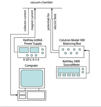
The data acquisition system for the ExB is shown in Figure 2.15. In this system, the potential for the electric field plates was supplied by a Keithley 2400 SourceMeter, and was balanced using the voltage balancing box supplied with the Colutron filter. A Keithley 6284A power supply was used to supply the DC current for the magnet coils. The collector current signal was sent to the computer and recorded, along with position information from the translation stage.
Keithley 2400 SourceMeter Colutron Model 300
Balancing Box Keithley 6284A Power Supply Computer co lle ct or c ur re nt m ag ne t c ur re nt po te nt ia ls fo r el ec tr ic fi el d vacuum chamber
0-20 V, 0-3 A Keithley 2400
SourceMeter Keithley 2400
SourceMeter Colutron Model 300
Balancing Box Colutron Model 300
Balancing Box Keithley 6284A Power Supply Keithley 6284A Power Supply Computer Computer co lle ct or c ur re nt m ag ne t c ur re nt po te nt ia ls fo r el ec tr ic fi el d vacuum chamber
[image:44.595.103.456.322.696.2]0-20 V, 0-3 A
2.4.3 Uncertainty Analysis
There were several sources of error and uncertainty in the ExB results, including internal CEX collisions, interactions between the probe and the thruster plume, and spread in the ion velocities due to collector and aperture sizing. As mentioned previously, there was a mesh-covered hole in the bottom of the ExB housing, so that neutrals could not build up inside the device. This was done to reduce neutral density inside the device, so that the high velocity Xe+ signal could not be attenuated due to CEX collisions between Xe+ and neutral Xe atoms. However, although this decreased the neutral density, it was impossible to completely eliminate the density of neutrals within the device. Because of the size of the hole, it was assumed that the density inside the device equilibrated to the background neutral density.
In the 650W case, the background density of neutrals was significantly higher than in the 200W case, as evidenced by a higher vacuum pressure within the chamber. Additionally, the background neutral density was likely higher near the exit plane of the thruster than far from it. This change in neutral density is hard to quantify without a direct measurement, but from a qualitative standpoint it is fair to say that there is likely greater signal attenuation at smaller axial distances, and also that the signal attenuation is more significant for the 650 W case.
It also should be mentioned that there was some unavoidable interaction between the probe housing and the thruster plume. Although attempts were made to minimize the surface area that was exposed to the thruster plume, for example by adding a conical taper to the front of the device, there was still visible interaction between the ion beam and the device. The other countermeasure that was taken was to reduce the amount of time that the probe spent in front of the thruster plume during the scan. A shorter time scale for the scan also helped to decrease the neutral buildup inside the device due to neutrals entering through the front aperture.
to the E/B value.
θ1 D2
L1 L2 L3 L4
θ2 Dc
D3 D4 L5 D5 D6 vz vy1 z y Ap er tu re 1 Ap er tu re 2 Ap er tu re 3 Co lle ct or Electrodes Ion Path
θ1 D2
L1 L2 L3 L4
θ2 Dc
D3 D4 L5 D5 D6 vz vy1 z y Ap er tu re 1 Ap er tu re 2 Ap er tu re 3 Co lle ct or Electrodes Ion Path
Figure 2.16: ExB resolution calculation
The spread in the data can be calculated as follows. First, start by calculating the maximum input angle, θ1, for ions:
θ1 =tan−1
D2 L1
. (2.3)
This allows the y-position of the ion at the entrance of the filter to be calculated (D3):
D3 = (L1+L2)tan(θ1). (2.4)
Then, by applying the Lorentz force equation (Eqn. 2.1) and assuming that acceleration in the z-direction is negligible, this allows the acceleration in the y-direction to be calculated:
ay =− q
m(E−vzB). (2.5)
Note that the ratio of E/B is set to measure a certain ion velocity:
vset = E
B. (2.6)
So Eqn 2.5 can be rewritten as:
ay =− q
The time it takes for the ion to transit the filter can be estimated by dividing the filter length by the axial velocity:
t3= L3
vz. (2.8)
If transit time and acceleration are known, then the position and velocity of the ion at the end of the filter can be calculated, as well as the value of θ2:
D4 =D3+ (vy1)t3+
1 2ayt
2
3 (2.9)
vy4 =vy1+ayt3 (2.10)
θ2 =tan−1
vy4 vz
. (2.11)
Finally, the y-position at the z-position of the third aperture (D5) and at the collector (D6) are:
D5 =D4+L4tan(θ2) (2.12)
D6 =D5+L5tan(θ2). (2.13)
In order for the ion to pass through the third aperture, the condition onD5 must be:
|D5| ≤ DA3+D2
2 , (2.14)
whereDA3is the width of the third aperture. Additionally, for the ion to hit the collector, the condition onD6 is:
|D6| ≤
Dc+D2
2 . (2.15)
2.5
Diagnostic Instruments - Retarding Potential Analyzer
2.5.1 Instrument Overview
A retarding potential analyzer (RPA) was used to take energy distribution measurements in the SPT-70 plume. A RPA is a parallel grid electrostatic analyzer that uses an applied potential (the ”retarding” potential) to accept or reject ions based on their energies. Fig-ure 2.17 shows a schematic of a typical RPA. The front grid is usually allowed to float at the plasma potential, while the ”screen” grid is biased at a low negative potential to keep out electrons. The ”retarding” grid potential is ramped from zero to several hundred or thousand volts, depending on the acceleration voltage of the thruster being examined. Sometimes, a ”suppressor” grid is used to prevent secondary electrons (i.e., electrons produced due to ions colliding with the collector) from causing a false current reading. A collector at the back of the device measures the ion current.
ions
co
lle
ct
or
front grid
retarding grid
screen grid
½mv2< qφ
ions
co
lle
ct
or
front grid
retarding grid
screen grid
½mv2< qφ
Figure 2.17: RPA Schematic.
The device operates on the principle of energy conservation:
1 2mv
2 =qφ. (2.16)
derivative of the raw data, also shown in Figure 2.18. Io n C urre nt (R aw D at a) Pr op or tion of Io n C ur re nt (D iff er en tia te d D at a)
Energy per Charge
Io n C urre nt (R aw D at a) Pr op or tion of Io n C ur re nt (D iff er en tia te d D at a)
Energy per Charge
Figure 2.18: RPA sample trace. Taking the derivative of the raw data gives the energy distribution.
One other point to note is that the RPA does not distinguish between charge species. According to Equation 2.16, a double ion must have twice the kinetic energy as a single ion to overcome the same potential barrier. However, using RPA data it is not possible to make the distinction between a single ion that is moving with a certain kinetic energy and a double ion that is moving with twice that energy.
2.5.2 Instrument Design and Data Acquisition System
The particular RPA used in the experiment employed 3 grids, as shown in Figure 2.19. The front grid was mounted so that it was flush with the face of the RPA housing. Both the front face and grid were electrically isolated from the body of the RPA, which was grounded. The screen grid was mounted 1 mm behind the front grid, and during operation was set at -20 V. Behind the screen grid was the ”retarding” grid, to which the voltage ramp was applied to decelerate ions entering the device. The spacing between the screen and retarding grids was 2.5 mm. The collector anode was located 1.0 mm behind the retarding grid.
retarding grid (0 to 102 or 103V) front grid (floating) screen grid (-20 V) IONS col le ct or insulating spacer RPA Dimensions:
Front grid to collector 4.5 mm Screen grid to collector 3.5 mm Retarding grid to collector 1.0 mm
fron t sc re en re tar d in g co lle ct
or Spacer inner diam. 14.3 mmSpacer outer diam. 23.1 mm front screen retarding collector
spacer 1 spacer 2 spacer 3 retarding grid (0 to 102 or 103V)
front grid (floating) screen grid (-20 V) IONS col le ct or insulating spacer RPA Dimensions:
Front grid to collector 4.5 mm Screen grid to collector 3.5 mm Retarding grid to collector 1.0 mm
fron t sc re en re tar d in g co lle ct
or Spacer inner diam. 14.3 mmSpacer outer diam. 23.1 mm front screen retarding collector
spacer 1 spacer 2 spacer 3 retarding grid (0 to 102 or 103V)
front grid (floating) screen grid (-20 V) IONS col le ct or insulating spacer
retarding grid (0 to 102 or 103V) front grid (floating) screen grid (-20 V) IONS col le ct or insulating spacer RPA Dimensions:
Front grid to collector 4.5 mm Screen grid to collector 3.5 mm Retarding grid to collector 1.0 mm
fron t sc re en re tar d in g co lle ct
or Spacer inner diam. 14.3 mmSpacer outer diam. 23.1 mm front screen retarding collector
spacer 1 spacer 2 spacer 3
Figure 2.19: RPA photo and schematic.
retarding grids were both made out of a stainless steel mesh, 0.2 mm thick, with an open area fraction of 0.36. These two grids were positioned such that the holes in the mesh were not aligned, to prevent secondary or tertiary alignment patterns (Moire patterns) depending on the angle of the device relative to the ion source. All of the grids had an outer diameter of 22 mm. The collector anode consisted of a 22 mm diameter, 0.1 mm thick, tungsten disk. The angle of acceptance of the device was 15 deg (full angle) and was determined experimentally [27].
The components of the RPA data acquisition system are shown in Figure 2.20. A standard DC power supply was used to apply a potential of -20 V to the screen grid, while a function generator plus a high-voltage amplifier were used to create the ramp voltage for the retarding grid. The current to the collector was amplified using a gain of 105 to 108, depending on the magnitude of the signal. The voltage from the signal generator was sent to the control computer through a data acquisition box, and this signal was synched to the acquisition of the current measurement. The resolution of the data acquisition system could be varied using a Labview control program.
SRS DS 345 Synthesized Function Generator Agilent E3647
Power Supply
DC, 0-35 V, 0.8 A KEPCO Bipolar OperationalPower Supply/Amp.
+/- 1000 V, +/- 40 mA Keithley 427
Current Amplifier
NI DAQPad-6052E
Computer vacuum chamber
retarding voltage screen voltage
collector signal
SRS DS 345 Synthesized Function Generator
SRS DS 345 Synthesized Function Generator Agilent E3647
Power Supply
DC, 0-35 V, 0.8 A Agilent E3647 Power Supply
DC, 0-35 V, 0.8 A KEPCO Bipolar OperationalPower Supply/Amp.
+/- 1000 V, +/- 40 mA KEPCO Bipolar Operational
Power Supply/Amp.
+/- 1000 V, +/- 40 mA Keithley 427
Current AmplifierKeithley 427
Current Amplifier
NI DAQPad-6052E NI DAQPad-6052E
Computer Computer vacuum chamber
retarding voltage screen voltage
collector signal
be determined at specific locations in the plume. See Section 2.6 for a description of the scans taken with the RPA.
2.5.3 Uncertainty Analysis
Uncertainty and errors in the RPA results comes from a number of sources, namely: charge exchange (CEX) collisions inside the device, ion optics of the grids, and the differentiation method that was used. In some of the RPA scans that are close to the thruster centerline (0 deg and 10 deg cases, for example, in Figures 5.16 and 5.19), one can see ions with energies per charge that are greater than the acceleration potential of the device. Theoretically, one should not see ions that have kinetic energies greater than that which can be obtained by acceleration though a certain potential drop (250 eV in the 200W case, 300 eV in the 650 W case).
One explanation for ions with energies per charge that are higher than the accel-eration potential is that these ions that have gone from Xe2+ to Xe+ in a CEX collision. Such ions can have an energy/charge greater than 300eV/q. If you look at the energy conservation equation (qφ = 1/2mv2), a doubly charged ion will have double the kinetic energy as a singly charged ion if accelerated through the same potential. In a CEX collision between a Xe2+ ion and a Xe atom in which two Xe+ are produced, one of the Xe+ ions will attain the kinetic energy of the Xe2+ ion after the collision, and thus will have twice the energy per charge as the Xe2+ ion.
Another source of uncertainty relates to the ion optics of the grids. As the potential on the retarding grid increases, a larger range of ion energies can be accepted through the grid holes due to the fact that the potential drops slightly within each hole. To simulate ion trajectories near a grid hole inside the RPA, a program called Simion was used [28]. Simion calculates the electrostatic potential distribution for a given configuration in 2D, and also simulates ion trajectories through the configuration. An example of a Simion calculation for the problem at hand is shown in Figure 2.21. This figure shows that the potential barrier is slightly lower within the hole, meaning that an ion with an energy per charge lower than the retarding potential can pass through it. The results of the Simion simulations are shown in Table 2.2. These results suggest that the uncertainty is roughly 2-3 percent of the applied retarding voltage.
Collect or (0 V
) Retard
ing Gri d Screen
Grid(-2 0V)
x y
φ
Ion Path
Collect or (0 V
) Retard
ing Gri d Screen
Grid(-2 0V)
x y
φ
Ion Path
Figure 2.21: Example result from Simion. The height of the graph represents the potential,φ. In this particular case the retarding potential was set to 200V, with the screen grid voltage at -20V and the collector at 0 V. The ion had an initial kinetic energy of 119.5 eV, which is lower than the 120 eV that would be needed to get over the potential barrier if the grid hole was not present.
Table 2.2: RPA uncertainty due to ion optics
Retarding Voltage [V]
Lowest Accepted Energy/Charge
[eV/q]
∆V [V]
Proportion of Retarding
Voltage
50 48.8 -1.2 0.024
100 97.8 -2.2 0.022
150 146.7 -3.3 0.022
200 195.7 -4.3 0.022
250 244.7 -5.3 0.021
300 293.5 -6.5 0.022
350 342.6 -7.4 0.021
400 391.5 -8.5 0.021
calculation. In this study, there was a sufficient amount of noise that some averaging of the raw data had to be done. It was found that an average over 20 points was sufficient. This, therefore, reduced the number of data points in the file from 10,000 to 500. Additionally the slope of the data at a given point was calculated using the following algorithm:
dI dV =
nP
VavgIavg−PVavgPIavg n
P
V2 avg−(
P Vavg)2
, (2.17)
where n is the number of data points over which the slope was calculated, and the sums are taken over each set of n data points, using the averaged current and voltage values (such that the center point of each sum is a data point in the differentiated data set). In the 200 W case it was determined that n=3 led to a differentiated curve with a satisfactory amount of smoothness, so after the differentiation the number of points in the data set was 166. In the 650 W case, it was necessary to set n = 5, so the number of points was reduced to 100. Since both scans were taken from -50 to 450 V, for a total change of 500 V, the uncertainties were 500/166 = 3.01 eV/q for the 200 W case and 500/100 = 5.00 eV/q for the 650W case.
2.6
Summary of Scans
set at zero and not changed due to its large angle of acceptance. Table 2.3 summarizes the data collected using the faraday probe.
In the case of the ExB filter, two types of scans were taken: transverse and axial. During a transverse scan, the axial location and angle was fixed and the probe was moved perpendicular to the thruster centerline. Because the angle of acceptance of the ExB filter was less than a degree, the probe angle was varied to determine the dependence of ion current on angle. During an axial scan, the transverse location was fixed and the probe was moved in the direction of the thruster, parallel to the thruster centerline. Table 2.4 summarizes the data collected using the ExB filter.
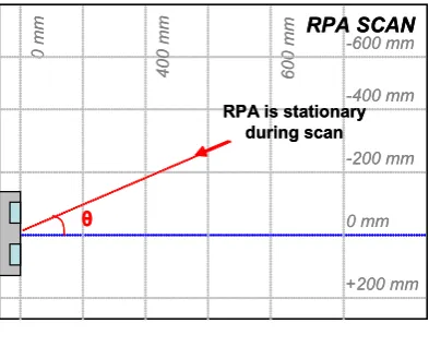
Unlike the other probes, the RPA could not be moved while it was taking data. Instead, it was positioned at a specific angle off of the thruster centerline, at a specific distance away from the thruster, as shown in Figure 2.23. For most of the scans, the distance was 400 mm, but in some cases the RPA had to be moved further away, to ensure that the device used to amplify its signal was not saturated, and also to prevent electrical shorts inside the probe. Table 2.5 summarizes the data collected using the RPA.
0 m m -200 mm +200 mm 0 mm 10 0 m m -400 mm θ tr an sv er se d ire ct io n TRANSVERSE SCAN (ExB and FP)
negative side positive side 0 m m -25 mm +25 mm 0 mm 20 0 m m -50 mm axial direction AXIAL SCAN (ExB only) 0 m m -200 mm +200 mm 0 mm 10 0 m m -400 mm θ tr an sv er se d ire ct io n TRANSVERSE SCAN (ExB and FP)
negative side positive side 0 m m -25 mm +25 mm 0 mm 20 0 m m -50 mm axial direction AXIAL SCAN (ExB only)
0 m m 60 0 m m -200 mm +200 mm 0 mm 40 0 m m -400 mm -600 mm θ RPA SCAN
RPA is stationary during scan 0 m m 60 0 m m -200 mm +200 mm 0 mm 40 0 m m -400 mm -600 mm θ RPA SCAN
RPA is stationary during scan
[image:56.595.182.379.175.334.2]Figure 2.23: RPA scans. During each scan, the RPA position was fixed.
Table 2.3: Summary of Faraday probe scans Thruster Operat-ing Point Axial Position [mm] Transverse Position [mm] Angle of Faraday Probe [◦]
Chamber Pressure [torr] Cathode Float Voltage [V] 200 W 15 to
1500
-477 to
223 0 3.0x10
−6 -14.0
650 W 15 to 1500
-477 to
223 0 6.5x10
Table 2.4: ExB scan summary Thruster Operat-ing Point Type of Scan Axial Position [mm] Transverse Position [mm] Angle of ExB Probe [◦]
ExB Setting Chamber Pressure [torr] Cathode Float Voltage [V]
200 W Trans.
50, 75, 100, 125, 150, 175, 200 -477 to 223 0, 10, 20, 30, 40, 50, 60, 70 ON (set at Xe+ location)
2.5x10⁻⁶ -15.4
200 W Trans.
50, 75, 100, 125, 150, 175, 200 -477 to 223 0, 10, 20, 30, 40, 50, 60, 70 OFF (no deflec-tion)
2.5x10⁻⁶ -15.4
650 W Trans.
50, 75, 100, 125, 150, 175, 200 -477 to 223
0, 10, 20, 30, 40
ON (set at Xe+ location)
6.0x10⁻⁶ -35.5
200 W Axial 400 to 50 -27, -4,
0, 23 0
ON (set at Xe+ location)
2.5x10⁻⁶ -15.4
200 W Axial 400 to 50 -27, -4,
0, 23 0
OFF (no
deflec-tion)
2.5x10⁻⁶ -15.4
650 W Axial 400 to 50 -27, -4,
0, 23 0
ON (set at Xe+ location)
6.0x10⁻⁶ -35.5
Table 2.5: RPA scan summary Thruster Operat-ing Point Distance from Thruster Center [mm]
Angle Off of Thruster Centerline [◦]
Chamber Pressure [torr] Cathode Float Voltage [V]
200 W 400
0, 10, 20, 30, 40, 45, 50, 55, 60, 65, 70, 75,
80, 85, 90
2.5x10⁻⁶ -15.0
650 W 400
45, 50, 55, 60, 65, 70, 75, 80,
85, 90
8.0x10⁻⁶ -14.0
650 W 600 10, 20, 30, 40,
45 8.0x10
−6 -14.0
Chapter 3
Simulation Approach - HPHall
In the simulation portion of this research, two approaches were used. The first was an existing hybrid-PIC Hall thruster code known as HPHall, which was used to investigate both the central jet and high angle, high energy ions. As was mentioned previously, internal hybrid-PIC codes only simulate a small portion of the near-field. Nonetheless, this type of model can still give insight into the acceleration of ions inside the channel and immediately outside the exit plane, even if it does not capture the full extent of the near-field region. Furthermore, a better alternative (such as a well-validated fully-kinetic or fluid-based model) was not readily available.
This chapter describes the simulation method used by the hybrid-PIC model. In the case of HPHall, since it was an existing code with a substantial development history, most of the information is summarized from other sources, with references provided as needed.
3.1
Hybrid-PIC Model Overview
As stated in the introduction, HPHall is a hybrid-PIC Hall thruster code that treats electrons as a fluid and ions as particles-in-cell. HPHall was first developed by J. M. Fife and M. Martinez-Sanchez at MIT during the mid-1990s [14]. In the ensuing years, it has gained wide acceptance by the Hall thruster research community. Currently, HPHall, as well as similar codes based on hybrid-PIC methods, are used by most institutions that engage in the modeling of these thrusters [15–18]. Although other approaches exist, such as pure fluid codes that model electrons and ions as fluids [29], and fully kinetic codes that handle both species using a particle-based method [30, 31], none are as widely used as hybrid-PIC.
M. Fife [14] (unless otherwise noted, the content of this section represents a summary of the information presented in this document). In spite of the modifications that have been made to HPHall since its initial creation, the basic solution method and assumptions have not changed. As illustrated in Figure 3.1, the basic method is as follows. First, the solution grid and magnetic field are generated by separate solvers outside of HPHall. These files are required by HPHall to initiate the solution process, as well as a third file that specifies the input parameters of the code. Initially, the solution domain is not populated by particles, unless files from a previous HPHall run are used. The grid, magnetic field, and input parameter information is then fed into the fluid solver and the solution process initiated.
During the solution process, HPHall integrates the electron fluid equations on a two-dimensional domain, then moves the ions based on the results from the electron sub-model. The major assumptions of the code are as follows: (1) the plasma is quasi-neutral (i.e., ne = nXe1+ + nXe2+), (2) the induced magnetic field is small compared to the applied field and can be neglected, (3) the problem is axisymmetric about the thruster centerline. Using these assumptions, the code simulates the plasma between two boundaries, the “anode line” and the “cathode line”. Both the anode and cathode “lines” correspond to λ-lines, the magnetic streamlines that will be described in the following sub-section. On these boundaries, plasma parameter values, such as potential and electron temperature, are specified. An example solution domain for the SPT-70 is shown in Figure 3.2.
3.1.1 Electron Sub-model
In the electron sub-model, the electrons are assumed to be strongly-magnetized, so electron motion can be split into two clear parts: motion along and motion across magnetic field lines. The magnetic field can be described using Maxwell’s equations:
∇ ·B~ = 0 (3.1)
∇ ×B~ =µ0
~j+0
∂E ∂t
≈0. (3.2)
Grid input file Magnetic field input file Parameter input file
Simulation initialization
Integrate electron equations (fluid equations)
Ohm’s Law Current Conservation Electron Temperature
Move heavy particles (particle-in-cell methods)
Ionize neutrals, inject neutrals at anode
Simulation Outputs
Δt = 2x10⁻¹⁰s
Δt = 5x10⁻⁸s
Te, φ
ni, ui nn, un Grid input file Magnetic field input file Parameter input file
Simulation initialization
Integrate electron equations (fluid equations)
Ohm’s Law Current Conservation Electron Temperature
Move heavy particles (particle-in-cell methods)
Ionize neutrals, inject neutrals at anode
Simulation Outputs
Δt = 2x10⁻¹⁰s
Δt = 5x10⁻⁸s
Te, φ
[image:60.595.86.474.215.587.2]ni, ui nn, un
Axial Location [m] R ad ia lL oc at io n [m ]
0 0.01 0.02 0.03 0.04 0.05
0 0.01 0.02 0.03 0.04 0.05 anode line cathode line insulating wall insulating wall
Axial Location [m]
R ad ia lL oc at io n [m ]
0 0.01 0.02 0.03 0.04 0.05
[image:61.595.132.513.77.377.2]0 0.01 0.02 0.03 0.04 0.05 anode line cathode line insulating wall insulating wall
Figure 3.2: SPT-70 solution domain. Cathode and anode lines correspond to magnetic streamlines known asλlines.
to the gradients in the magnetic field. Based on these equations, one can define a mag-netic potential function, σ, and a magnetic stream function, λ, that satisfy the following relationships.
~
B =∇σ (3.3)
∇2σ= 0 (3.4)
across λ-lines.
The derivation of the electron equations, as well as the integration method, is fairly complicated. Rather than describe the specifics here, the reader is instead referred to Fife’s PhD thesis [14].
3.1.2 Heavy Particle Sub-model
In the heavy particle sub-model, a separate simulation mesh is used to calculate particle motion. Rather than advance the particles in physical space directly, the problem is first transferred to a simpler domain. The relatively complicatedr−zmesh shown in Figure 3.3 is transformed to a rectangularξ−η mesh, whereξandηare represented by integer values, as shown in Figure 3.3. The particle positions, velocities, and forces are also transformed to the ξ−η plane. Particle motion is then calculated on this plane, and transf


![Figure 3.1: HPHall program flow. This graphic has been modified from one appearing in [14]](https://thumb-us.123doks.com/thumbv2/123dok_us/16871.1243/60.595.86.474.215.587/figure-hphall-program-ow-graphic-modied-appearing.webp)


