UNIVERSITY OF SOUTHERN QUEENSLAND FACULTY OF ENGINEERING AND SURVEYING
Supercritical
Carbon Dioxide
Geothermal Energy
System Analysis
A dissertation submitted by
Mr Patrick Taylor
In fulfillment of requirements of
Bachelor of Engineering (Mechanical)
i
ABSTRACT
There has been considerable interest in the possibility of using supercritical carbon dioxide (SCCO2) as a geothermal heat mining fluid instead of water. Some
favourable fluid transport properties may prove to give an advantage in some circumstances. The low viscosity to density ratio suggests higher mass flow rates and better suitability to low permeability reservoirs may be possible. Higher frictional losses in the wellbores may degrade that advantage.
It has been shown that SCCO2 has the potential to utilise buoyancy effects such that
a thermosiphon circulates the geothermal fluid without the need for a pump. In addition, it has been proposed that SCCO2 could be used to drive a turbine directly
rather than a conventional binary heat exchange system. This could dramatically reduce surface plant complexity and cost.
This study details the creation of a Matlab model of the subsurface circuit of geothermal fluid. After establishing a reference case to study general fluid and system behaviour, the model is used to test and compare the effects of wellbore diameter variation, reservoir depth, permeability and temperature on the net exergy and thermal efficiency using each of water and SCCO2.
For the specific test cases, SCCO2 was shown to perform significantly better than
water with increased well bore diameter, low permeability and low temperature reservoirs. The performance was found to degrade with shallower reservoirs; although this leads to observations that the SCCO2 system operates on a narrow
ii
DISCLAIMER
University of Southern Queensland
Faculty of Health, Engineering and Sciences
ENG4111/ENG4112 Research Project
Limitations of Use
The Council of the University of Southern Queensland, its Faculty of Health, Engineering & Sciences, and the staff of the University of Southern Queensland, do not accept any responsibility for the truth, accuracy or completeness of material contained within or associated with this dissertation.
Persons using all or any part of this material do so at their own risk, and not at the risk of the Council of the University of Southern Queensland, its Faculty of Health, Engineering & Sciences or the staff of the University of Southern Queensland.
iii
CANDIDATES CERTIFICATION
I certify that the ideas, designs and experimental work, results, analyses and conclusions set out in this dissertation are entirely my own effort, except where otherwise indicated and acknowledged.
I further certify that the work is original and has not been previously submitted for assessment in any other course or institution, except where specifically stated.
Patrick Taylor
Student Number: 0019522109
__________________________
iv
ACKNOWLEDGEMENTS
I would like to thank…
• Dr Ruth Mossad for her valuable input and guidance on this project.
• Dr David Fletcher for his patient and valuable advice on the CFD modelling.
• Most of all I am grateful to my eternally patient wife Arna, my two protégé’s Joel and Nyah who have endured the ups and downs of 8 years study with grace and understanding.
v
TABLE OF CONTENTS
Abstract ... i
Disclaimer ... ii
Candidates Certification ... iii
Acknowledgements ... iv
Table of Contents ... v
List of Figures ... viii
List of Tables ... x
Glossary and Acronyms ... xi
1 Introduction ... 1
1.1 Background ... 1
1.2 Geothermal Energy Overview ... 2
1.2.1 Types of Geothermal Energy Utilisation ... 3
1.2.2 Geothermal Electricity Production Cycles... 5
1.2.3 Well Drilling ... 7
1.2.4 Geothermal Resources ... 8
1.3 Research Objectives ... 10
2 Literature Review ... 11
2.1 Supercritical CO2 System Operation Overview ... 11
2.1.1 System Overview ... 11
2.1.2 Supercritical Carbon Dioxide ... 13
2.2 Previous Studies on SCCO2 EGS ... 14
3 Research Design and Methodology ... 17
3.1 Introduction ... 17
3.2 Methodology ... 17
3.3 Assumptions ... 18
3.4 Parametric Study Design ... 19
3.4.1 Reference Case ... 20
3.4.2 Parametric Investigation ... 24
3.5 System Mathematical Model ... 26
3.5.1 Model Overview ... 26
vi
3.5.3 CO2 Property Model ... 29
3.5.4 Water Property Model ... 35
3.5.5 Preliminary System Estimates – CO2 ... 35
3.5.6 Preliminary System Estimates - Water... 37
3.5.7 Wellbore Pressure Gradient ... 39
3.5.8 Wellbore Heat Transfer ... 40
3.5.9 Reservoir Fluid State ... 42
3.5.10 Turbine Power Output (CO2) ... 43
3.5.11 Cooling Tower Heat Extraction (CO2) ... 43
3.5.12 Heat Exchanger Energy Extraction (Water) ... 43
3.5.13 Pumping Power Input (Water) ... 43
3.5.14 Energy Balance ... 43
3.6 Performance Comparison ... 44
3.6.1 Exergy ... 44
3.6.2 Thermal Efficiency ... 45
3.7 CFD Analysis ... 46
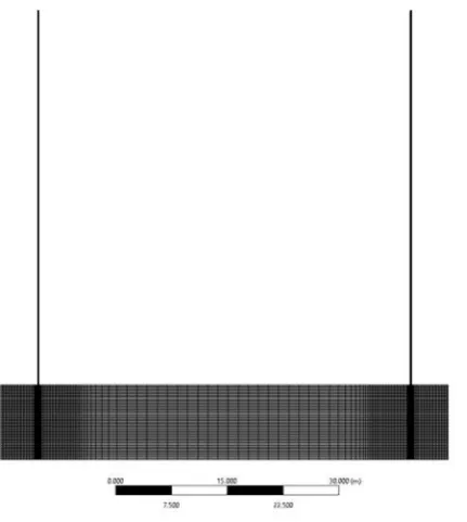
3.7.1 CFD Model Geometry ... 47
3.7.2 CFD Model Mesh ... 47
3.7.3 CFD Model Analysis Settings ... 49
4 Results and Discussion ... 52
4.1 Fluid Property Behaviour ... 52
4.2 Reference Case ... 57
4.2.1 Carbon Dioxide Single Loop – Thermosiphon Limited ... 57
4.2.2 Carbon Dioxide Single Loop – Friction Limited ... 60
4.2.3 Water Based Binary – Friction Limited ... 62
4.2.4 Carbon Dioxide Reference Case Final ... 64
4.2.5 Water Based Binary – Reference Case Final ... 65
4.3 Effect of Wellbore Diameter Variation ... 66
4.4 Effect of Reservoir Depth Variation ... 69
4.5 Effect of Reservoir Permeability Variation ... 72
4.6 Effect of Reservoir Temperature Variation ... 74
vii
5.1 Overall Findings ... 76
5.1.1 Model Uncertainty ... 76
5.1.2 Parametric Test Outcomes ... 76
5.1.3 CFD Analysis Outcomes ... 77
5.2 Further Work ... 78
Appendix A – Project Specification ... 79
Appendix B – Reference Case Parameter Sources ... 81
Appendix C – Matlab Script ... 83
Geothermal_Main ... 83
Geothermal_CO2.m ... 86
CO2_Prop.m ... 93
Geothermal_Water.m ... 97
XSteam.m ... 103
viii
LIST OF FIGURES
Figure 1-1 - Global Carbon Cycle Components (U.S. Department of Energy
Genomic Science 2008) ... 1
Figure 1-2 - Diagram of the earth's structure ... 2
Figure 1-3 - Home Heating With a Geothermal Heat Pump System (GeoExchange 2011) ... 4
Figure 1-4 - Indicative thermal gradient at shallow depths (Solarpraxis 2014) ... 4
Figure 1-5 - Geothermal Power plant Basic Schematic (EPA 2013) ... 5
Figure 1-6 - Representative geothermal well design (Gurgenci 2011) ... 7
Figure 1-7 - EGS System Diagram (Dorminey 2012)... 9
Figure 2-1 - Concept for geothermal plant designs. (Atrens, Gurgenci & Rudolph 2008) ... 11
Figure 2-2 - Carbon dioxide pressure-temperature phase diagram ... 14
Figure 3-1 - Matlab Script Hierarchy ... 27
Figure 3-2 - CFD Model Geometry ... 47
Figure 3-3 - CFD Model Mesh - Overview ... 48
Figure 3-4 - CFD Model Mesh - Reservoir Inlet Region ... 48
Figure 3-5 - CFD Model Mesh - Injection well inflation and domain interface. ... 49
Figure 3-6 - Trial CFD model fluid flow - CO2 into the reservoir ... 50
Figure 3-7 - Trial CFD model fluid flow - CO2 into the reservoir ... 50
Figure 3-8 - Trial CFD model fluid flow - CO2 into the reservoir ... 51
Figure 4-1 - CO2 system injection well – typical fluid property variation ... 53
Figure 4-2 - CO2 system reservoir – typical fluid property variation ... 53
Figure 4-3 - CO2 system production well – typical fluid property variation ... 54
Figure 4-4 - Specific heat capacity vs temperature non-linearity ... 55
Figure 4-5 – Water system injection well fluid – typical property variation ... 56
Figure 4-6 – Water system reservoir fluid – typical property variation ... 56
Figure 4-7 – Water system production well – typical fluid property variation ... 57
Figure 4-8 – Mass flow rate vs injection pressure - limited by energy balanced thermosiphon (no pump). ... 58
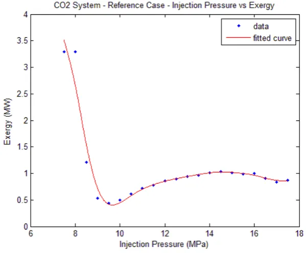
Figure 4-9 - Exergy vs injection pressure - limited by energy balanced thermosiphon (no pump). ... 58
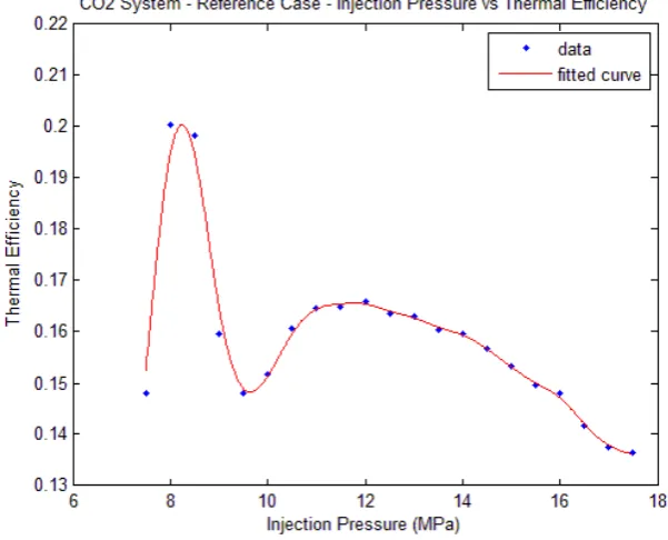
Figure 4-10 - Thermal efficiency vs injection pressure - limited by energy balanced thermosiphon (no pump). ... 59
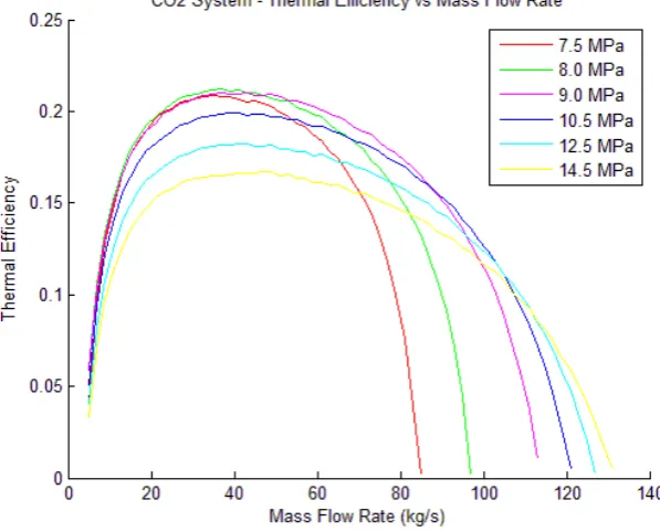
ix Figure 4-12 - Thermal efficiency vs mass flow rate limited by system
impedance (pumped flow - production well minimum pressure
constraint). ... 61 Figure 4-13 - Exergy vs mass flow rate limited by system impedance
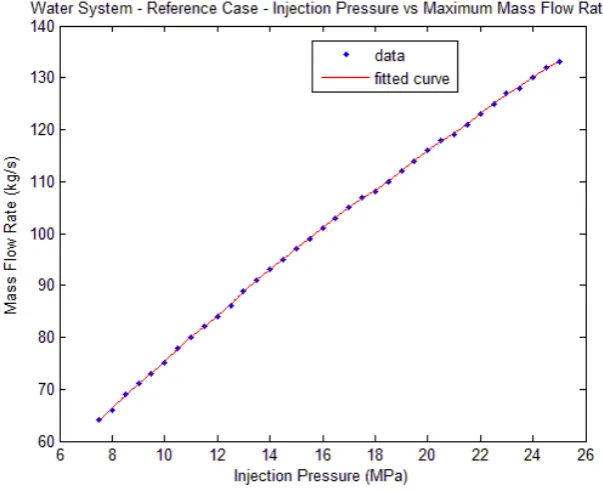
(pumped flow - production well minimum pressure constraint). ... 61 Figure 4-14 – Maximum mass flow rate vs injection pressure - limited by
system impedance (pumped flow - production well minimum
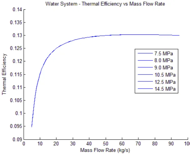
pressure constraint). ... 62 Figure 4-15 - Thermal efficiency vs mass flow rate limited by system
impedance (pumped flow - production well minimum pressure
constraint). ... 63 Figure 4-16 - Exergy vs mass flow rate limited by system impedance
(pumped flow - production well minimum pressure constraint). ... 63 Figure 4-17 - Exergy vs mass flow rate for the reference case injection
pressure of 10 MPa ... 66 Figure 4-18 – Mass flow rate vs pipe diameter for water and SCCO2 systems ... 66
Figure 4-19 – Net exergy vs pipe diameter for water and SCCO2 systems ... 67
Figure 4-20 – Thermal efficiency vs pipe diameter for water and SCCO2
systems ... 67 Figure 4-21 – Power loss from friction vs pipe diameter for water and
SCCO2 systems ... 68
Figure 4-22 – Mass flow rate vs reservoir depth for water and SCCO2
systems ... 69 Figure 4-23 – Net exergy vs reservoir depth for water and SCCO2 systems ... 69
Figure 4-24 – Thermal efficiency vs reservoir depth for water and SCCO2
systems ... 70 Figure 4-25 – Pressure at production well head vs reservoir depth for water
and SCCO2 systems ... 70
Figure 4-26 – Mass flow rate vs reservoir permeability for water and SCCO2
systems ... 72 Figure 4-27 – Net exergy vs reservoir permeability for water and SCCO2
systems ... 73 Figure 4-28 – Thermal efficiency vs reservoir permeability for water and
SCCO2 systems ... 73
Figure 4-29 – Mass flow rate vs reservoir temperature for water and SCCO2
systems ... 74 Figure 4-30 – Net exergy vs reservoir temperature for water and SCCO2
systems ... 75 Figure 4-31 – Thermal efficiency vs reservoir temperature for water and
x
LIST OF TABLES
Table 3-1 - Matlab Script File Functional Descriptions ... 28
Table 4-1 - Reference Case Data – SCCO2 ... 64
Table 4-2 - Reference Case Data – Binary Water System ... 65
xi
GLOSSARY AND ACRONYMS
CFD Computational Fluid Dynamics
EGS Enhanced (or Engineered) Geothermal System – refers to a
system with an artificially stimulated reservoir.
EOS Equation of State
Exergy (net exergy) Defined as usable energy or available energy.
Interchangeably used in terms of power. In this study, net exergy refers to the exergy measured in terms of fluid state potential minus the parasitic pumping power.
Flashing The changing of phase from liquid to steam in a well bore.
Geothermal Fluid The fluid which is pumped underground to transport heat energy to the surface for conversion to useful power.
GHP Geothermal Heat Pump
HDR Hot Dry Rock – refers to deep impervious granite
geothermal reserves (typically >4km under the surface)
Injection well The drilled and lined well through which the geothermal fluid flows from the surface to the reservoir.
Production well The drilled and lined well through which the heated geothermal fluid flows from the reservoir to the surface.
Reservoir The geological formation underground which contains the heat energy to be mined.
SCCO2 Supercritical Carbon Dioxide
Stimulation The act of injecting high pressure fluid into impervious or low porosity rock to create or increase fractures so that flow of the geothermal fluid is optimised.
Surface plant The collective name for all energy conversion equipment required at the surface to extract heat from the geothermal fluid and convert it to useful power.
1
1
INTRODUCTION
1.1
Background
It is almost universally acknowledged that humankind’s current dependence on the combustion of carbon based fuel for energy is not sustainable. This is most obviously due to the finite fossil fuel resources available; the rate of natural production of fossil fuels is many orders of magnitude slower than the rate of human consumption. Therefore, alternate, renewable energy sources need to be developed to replace fossil fuels which will eventually expire.
In addition, the effects of burning fossil fuels on the environment are becoming apparent and measurable. Carbon dioxide (CO2) is a primary product of
combustion. It is a known greenhouse gas; i.e. helps trap heat in the earth’s atmosphere which is essential to life as we know it. The current scientific position (again, almost universally) is that the amount of carbon dioxide directly or indirectly released by human activity is affecting the natural carbon system balance. Figure 1-1 shows this schematically. In simple terms, the result of this imbalance is an increase in atmospheric CO2 concentration and therefore an increase in the natural
[image:13.595.133.504.435.725.2]“greenhouse effect” and average surface temperature over time. This global temperature increase is enough to have adverse effects on the balance of many natural systems.
2 There is a wide body of readily available scientific literature, for example IPCC (2014), on global warming and the role of fossil fuel combustion. For the purpose of this project, it is taken as accepted knowledge that global warming is occurring and to some extent caused by human activity. This is important in so far that it is the fundamental principle driving the research and development of alternative, sustainable energy sources such as wind, solar and hydropower. Geothermal energy is also a sustainable resource with large but yet to be realised potential.
1.2
Geothermal Energy Overview
Geothermal energy is heat from the earth itself. This heat energy can be used either directly heating water or buildings or indirectly to generate electricity. It is considered to be in under the umbrella of renewable resources although, strictly speaking, due to the scale of this energy (the heat of the earth itself) is so large that it can be considered infinite (rather than having a capability to be renewed). Yusaf, Goh and Borserio (2011) agree with this perspective. A partial exception to this is in the case of utilising “hot dry rock” technology where the heat in deep granite is regenerated by radioactive decomposition of elements such as uranium, thorium and potassium isotopes. The rate of heat regeneration is still slow compared to the rate of heat extraction.
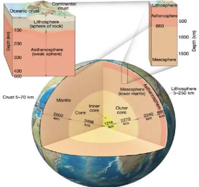
[image:14.595.218.418.532.720.2]DiPippo (2012) makes the comparison between the thickness of the earth’s crust and the shell of an egg. Proportionally, the thickness of an eggshell is three times that of the lithosphere (the earth’s crust). Considering the next region, the asthenosphere, is a semi molten layer averaging about 80km below the earth’s surface, one can expect there is a natural thermal gradient through the lithosphere and that the deeper we go, the hotter the rocks. Figure 1-2 shows the structure of the earth’s crust.
3
1.2.1 Types of Geothermal Energy Utilisation
Renewable Energy World (2014) and the Geothermal Energy Association (2014) provides a layman’s overview of the types of geothermal energy utilisation which are briefly presented here for contextual reference.
1.2.1.a Geothermal Direct Use
Regions which are near the earth’s plate boundaries or other volcanic activity often have shallow access to hot regions due to a naturally thin region of crust and fractures at plate boundaries. The historic utilisation of geothermal energy has been by direct use of hot water and/or rocks in these geologically active regions. For thousands of years, water from hot springs and surrounding heated rock has been used for cooking, heating and bathing. In more recent times, the heat has been used directly for industrial processes, heating buildings and many similar applications where low grade heat can be utilised directly. Accessing this energy resource can be very cheap and with a low impact on the environment however it is inherently restricted to geologically active regions. In addition, near surface regions are usually a low enthalpy resource – i.e. the temperature difference between the accessible resource and the surface is generally low. Considering that in any thermodynamic system the rate of heat (energy) transfer is proportional to the difference in absolute temperature, this is an important detail which directly impacts the viability of generating electricity.
1.2.1.b Geothermal Heat Pumps
4
Figure 1-3 - Home Heating With a Geothermal Heat Pump System (GeoExchange 2011)
[image:16.595.182.456.455.733.2]5 A GHP system can be more financially efficient in heating or cooling a building space than an equivalent electric or gas system because the heat energy comes from the ground. The only energy input is the pumping of the geothermal fluid and the compression of the vapour cycle gas. GHP systems are classified as low enthalpy due to the relatively low operating temperature of the resource being utilised.
1.2.1.c Geothermal Electricity Production
The geothermal systems that are designed to be of a scale to generate base load power (i.e. the heat energy is used explicitly to generate electricity) are the systems of interest in this project. There are several different types of plant system; all of which share the same desired output of a high pressure gas (or fluid) to drive a turbine. The turbine drives a generator to produce useable electricity to either feed into a power grid, or for direct use by industry (especially in remote locations). Figure 1-5 shows an extremely basic overview of a geothermal power plant. This will be expanded on significantly in following sections.
Figure 1-5 - Geothermal Power plant Basic Schematic (EPA 2013)
1.2.2 Geothermal Electricity Production Cycles
Some commonly used nomenclature for all these systems are introduced here;
• Production well - is the passageway (usually drilled) out of which the heated geothermal fluid flows.
• Injection well – is the passageway (usually drilled) through which the geothermal fluid is reinjected into the geothermal reservoir after the heat has been extracted.
6 or by natural reduction of pressure head as the fluid nears the surface. The flash steam is the “useful” component for electricity generation.
• Brine – refers to the fluid component of the geothermal fluid after the flash steam is removed.
The type of plant selected to achieve this depends on the type of geothermal resource being utilised. Briefly, there are four main types of commercial power plant. Renewable Energy World (2014) lists three:
a) Flash power plants, b) Dry steam power plants, c) Binary cycle power plants
and Geothermal Energy Association (2014) includes a fourth combination:
d) Flash/binary combined.
1.2.2.a Flash Power Plants
Flash power plants are the most common systems used in geothermally active regions. Hot water flows up though the production well and “flashes” at some point to become a mixture of hot water (brine) and flash steam. The flash steam is separated from the brine and used to drive a turbine. The brine (and condensate from the used flash steam) is reinjected to the geothermal reservoir. Fluid temperatures of above 180°C are generally required for flash systems (Renewable Energy World 2014).
1.2.2.b Dry Steam Power Plants
Dry steam power plants can be used if the geothermal resource produces steam directly from the production well. The system is schematically very simple as the steam directly drives a turbine to generate electricity. This type of system is rare in practice due to the limited available resource quality. For example Renewable Energy World (2014) say that there are only two known underground resources capable of producing dry steam in the United States, one of which is Yellowstone National Park and is protected from development.
1.2.2.c Binary Cycle Power Plants
7 have a lower boiling point than water – often an organic fluid such as isobutane or pentafluoropropane (Geothermal Energy Association 2014). As such, the “flashing” of the secondary fluid can be used to drive a turbine and generate power in the same way as steam, but at a lower temperature.
1.2.3 Well Drilling
The art and science of well drilling is not directly relevant to the scope of this project. However, since an arbitrary well geometry will form part of the system analysis model, it is important to note the shape of a deep well (up to 5km depth for an HDR EGS) may not be perfectly cylindrical. It is made up of a series of reducing pipe diameters as shown schematically in Figure 1-6.
Figure 1-6 - Representative geothermal well design (Gurgenci 2011)
Some additional well nomenclature;
• Casing – the surface lining of the drilled hole – usually concrete. Casing diameter is the effective flow cross-sectional area at a given point.
• String – refers to a length of section of the same diameter. Referring to Figure 1-6, there are 5 “strings”, the largest diameter at the top and the smallest diameter at the bottom.
8 production casing diameters may be 200mm to 340mm (Finger & Blankenship 2010).
1.2.4 Geothermal Resources
1.2.4.a Traditional Hydrothermal Geothermal Resources
Traditional geothermal systems rely heavily on a naturally occurring set of phenomena which are required in combination to create a useful source of geothermal energy. DiPippo (2012) describes the conditions required for a given region to be considered useful in a hydrothermal geothermal energy generation capacity as:
a) A large heat source, b) a permeable reservoir, c) a supply of water,
d) an overlying layer of impervious rock , e) a reliable recharge mechanism.
This is reasonably intuitive when considering the basic schematic shown in Figure 1-5. It can be seen that a geothermal energy system fundamentally operates by forcing a working fluid through a permeable layer of hot underground rock and extracting that heat at the surface for power generation. The quality of the heat source (temperature and overall heat capacity) directly affects the system performance.
The permeability of the geothermal reservoir must be such that the working fluid can pass through with a minimal pressure drop, but with enough time and mixing so that heat energy is fully absorbed by the fluid. To an extent, the permeability of an underground region can be improved by hydraulic fracturing. This is achieved by the injection of high pressure fluid into a region to increase the size of natural fractures.
An overlying layer of impervious rock is a requirement to provide some directional control for the geothermal fluid. Without this, the water/steam would dissipate slowly over an area rather than being channelled through a passage with a pressure and flow-rate that is useful.
A supply of naturally available water is usually requirement to provide a heat transfer medium to the surface and must be able to be replenished to account for losses in what will always be a non-sealed system (DiPippo 2012). A focus of this project is to consider supercritical carbon dioxide (SCCO2) as an alternative working
9 Traditionally, this set of conditions has significantly reduced the regions which could be considered to have geothermal energy production potential to those readily identified by observing natural hot springs, geysers and other surface activity.
1.2.4.b Enhanced Geothermal Systems (EGS) – Hot Dry Rock (HDR)
In areas which do not have a permeable pathway or readily available underground aquifers, a Hot Dry Rock (HDR) Enhanced Geothermal System (EGS) is a relatively new way of exploiting heat energy from the earth. This system concept is central to the focus of this project. Referring to the five conditions of a traditionally viable geothermal resource (in 1.2.4.a preceding), it can be seen that conditions (a) and (d) are a fundamental requirement. Condition (b), a permeable layer, can be man-made and this is the basis of an EGS system.
Figure 1-7 (Dorminey 2012) shows the basic layout of an EGS system. It is virtually identical to the traditional system shown in Figure 1-5; the critical difference is the hot granite being used as the heat source. This is important as granite is not permeable other than for some small fractures and discontinuities. For an EGS system to operate, the natural fractures must be “enhanced” with hydraulic fracturing techniques. This usually entails forcing water into the reservoir at high pressure in an incremental manner until the desired permeability and fracture field is achieved.
Figure 1-7 - EGS System Diagram (Dorminey 2012)
10 mostly due to development in deep drilling capability, EGS is been considered to have increasing commercial viability (Bahadori, Zendehboudi & Zahedi 2013).
Engineered Geothermal Systems (EGS) are the sole focus of this study; most specifically, analysis of the supercritical carbon dioxide (SCCO2) geothermal fluid
concept. At the time of writing there have been no working instances of an SCCO2
EGS trialled; even at pilot scale.
1.3
Research Objectives
Following from the background information, the objectives of this project are to:
1. Investigate the feasibility of using SCCO2 as a geothermal heat mining fluid
in a deep granite EGS.
2. Create a mathematical model of the wellbore and geothermal reservoir and compare SCCO2 with water as a geothermal heat mining fluid.
3. Develop a Matlab program using the mathematical model to investigate the parameters that affect its performance.
4. Validate the model with a CFD analysis of system components.
11
2
LITERATURE REVIEW
2.1
Supercritical CO
2System Operation Overview
2.1.1 System Overview
The concept of using SCCO2 as a geothermal working fluid was first proposed by
Brown (2000) in the paper “A Hot Dry Rock Geothermal Energy Concept Utilising Supercritical CO2 Instead of Water” presented to the Twenty-Fifth Workshop on Geothermal Reservoir Engineering at Stanford University, California. His paper is the foundation stone for this project and much previous work by others to investigate the feasibility of using SCCO2 as a geothermal heat mining fluid. Figure
2-1 (Atrens, Gurgenci & Rudolph 2008) shows a side by side comparison of a conventional water based binary EGS and a proposed SCCO2 thermosiphon design.
a) Traditional water-based binary plant design with associated organic Rankine cycle. Fluid flow from reference point 1 → 2 indicate injection well, 2 → 3 the reservoir, 3 → 4 the production well, 4 → 5 the heat extraction, and 5 → 1 the water pump for compression to injection pressure.
b) CO2 thermosiphon design. Fluid flow from reference point 1 → 2 indicate injection well, 2 → 3 the reservoir, 3 → 4 the production well, 4 → 5 the turbine, and 5 → 1 the cooling system.
12 With reference to Section 1.2.4.a and the list of conditions required for geothermal energy generation, the idea using of SCCO2 as a geothermal fluid in an EGS was
conceived to address the requirement for large volumes of water for both initial filling of the reservoir and ongoing replenishment of the inevitable losses during operation (Pruess 2006). Investigation of the concept has revealed several additional attractive features of SCCO2 that justify further investigation and
analysis.
Brown (2000), Pruess (2006) and Atrens, Gurgenci and Rudolph (2008) all agree on the following attractive features of the concept which include:
1. The reduced requirement for large volumes of water – especially attractive where HDR regions are far from water supplies (e.g. the Cooper Basin in Australia); making almost any location a potential site for geothermal plant. The requirement for large volumes of water in both initial filling of a reservoir and ongoing replenishment of the inevitable losses during operation can be a significant problem (Pruess 2006). Atrens, Gurgenci and Rudolph (2008) refer to potential steady losses in the order of 10%. Brown (2000) notes that SCCO2 can be used as the hydraulic fracturing fluid during
reservoir.
2. The properties of a supercritical fluid (discussed in detail in later sections) lead to a large pressure difference between the injection well and the production well. The difference is of a magnitude such that the system can operate on buoyant forces alone (a thermosiphon) – the potential is that no pumping is required (Atrens, Gurgenci & Rudolph 2010; Brown 2000; Pruess 2006) as shown schematically in Figure 2-1.
3. The rapidly expanding SCCO2 can be used to drive a turbine directly, much
like dry steam in a conventional system. This could lead to significantly reduced plant complexity and cost. In addition, a source of energy transmission loss, at the heat exchanger of a binary system, is removed. 4. The viscosity to density ratio of SCCO2 is lower than water allowing for a
larger mass flow rate for a given reservoir. This is offset somewhat by a lower specific heat capacity; however it is estimated to result in roughly equivalent energy generation capacity between water and SCCO2.
5. SCCO2 does not readily dissolve minerals. This is a major issue in geothermal
systems with water resulting in scaling and deposits, reducing the efficiency of pipes, heat exchangers and other related plant.
13 commodity in the future, the value of the carbon sequestration may help reduce the cost per MW and increase the attractiveness of the investment (Pruess & Azaroual 2006)
There have been some drawbacks identified with the SCCO2 concept. Most of the
earlier studies (identified by the author as prior to 2009) have significant simplifying assumptions. None appear to be unreasonable in the context of the respective papers; however, neglecting friction losses was a common feature. Atrens, Gurgenci and Rudolph (2009) found in their paper that the frictional losses in the pipe were a dominant factor in an exergy analysis. They found large gains linked to increasing the well bore diameter in an SCCO2 EGS model (the effect of which is reducing the
ratio of frictional losses at the boundary region). This is an easy adjustment from an academic perspective, however considering the drilling costs associated with an increased well bore diameter and the fact that the wellbores form the majority of construction cost (DiPippo 2008), this may not be a practical approach when cost analysis is inevitably applied.
The major and less tangible drawback is uncertainty. No such system has yet been constructed even at a pilot scale.
2.1.2 Supercritical Carbon Dioxide
A supercritical fluid is any substance held above a critical temperature and pressure at which it exists in a “4th state” (solid, liquid and gas being the traditionally recognised three). The supercritical state can be thought of as partway between liquid and gas, behaving in a homogenous way, but more like one or the other depending on the temperature and pressure. Some defining properties include:
• Supercritical fluid is compressible – changes in pressure or temperature result in large changes in density. It expands to fill its container like a gas.
• In general, the density of the supercritical fluid is close to that of a liquid.
• Supercritical fluid can dissolve materials like a liquid.
• It can diffuse through solids like a gas.
• There is no surface tension since there is no liquid/gas boundary.
14
Figure 2-2 - Carbon dioxide pressure-temperature phase diagram
The physical and thermodynamic properties of SCCO2 can be calculated by various
equations of state (EOS) with differing accuracies and levels of computational complexity. Heidaryan and Jarrahian (2013) explains that the van der Waals equation of state was developed in 1873 to improve the accuracy of the ideal gas law. Redlich and Kwong developed an improved equation of state by introducing temperature dependence. Peng and Robinson (1976) proposed additional modifications for more accuracy. Various improvements to these EOS have been developed to improve accuracy in certain areas of interest – for example behaviour close to the critical point. The Peng Robinson EOS and its derivatives are widely used in industry and are less computationally complex than its successors.
Span and Wagner (1996) proposed a new EOS for carbon dioxide; it is a modified version of the Helmholtz energy functions. Critical transport and thermodynamic properties specifically for CO2 have been calculated from the equations of state and
published on isobaric tables in their paper “A New Equation of State for Carbon Dioxide” (1996). The tables are very easy to use for simple calculations however the equations from which they are derived contain in the region of 50 terms. This makes coding of the Span and Wagner EOS cumbersome at best. The Peng Robinson EOS is significantly more straightforward with similar levels of accuracy in the context of this project.
2.2
Previous Studies on SCCO
2EGS
There have been a succession of analyses conducted on the SCCO2 EGS concept
15
• Confirmed the possibility of the SCCO2 system generating sufficient buoyant
forces to circulate without a pump.
• Temperature increase due to compression of SCCO2 is likely to increase the
temperature of the fluid by about 25°C; reducing thermal efficiency and buoyant forces. An increase in temperature at the injection well reduces the capacity to mine heat from the reservoir.
• For a given total pressure drop between injection and production wells, SCCO2 will generate approximately four times the mass flow and 50% larger
net heat extraction than water.
• The advantages of SCCO2 over water for energy extraction become more
pronounced with reduced temperature.
It is noted that frictional and inertial pressure gradients are neglected in these analyses.
Gurgenci et al. (2008) in the paper “Challenges for Geothermal Energy Utilisation”
propose that an SCCO2 EGS could operate on either a Rankine cycle or a Brayton
cycle. In the case of the former, the CO2 in cooled through a condenser to below
sub-critical state before reinjection. The Brayton cycle maintains the CO2 in
supercritical state throughout the circuit. Gurgenci et al. calculate the thermal efficiency of the Rankine cycle to be 29.5% and the Brayton to be 23.5%. However, it is noted that the Rankine cycle is not feasible for CO2 where ambient
temperatures rise above the supercritical point of 31°.
Atrens, Gurgenci and Rudolph (2008) conducted a similar analysis to Pruess (et al.) using Matlab to compare a SCCO2 thermosiphon and equivalent water based
system (refer to Figure 2-1). It is noted that frictional and inertial pressure gradients are neglected in these analyses. And the results are summarised as:
• SCCO2 and water systems produced approximately the same net power
output; 17MW vs 18MW respectively, based on the arbitrary parameters selected for the study.
• The slightly lower production of the SCCO2 system is somewhat offset by a
significant reduction in complexity of surface plant requirements. SCCO2
systems do not require pumping equipment or any secondary heat exchange system.
• In addition, the turbine is likely to be approximately half the size (and cost) of an isopentane turbine and approximately equal to a steam turbine.
An exergy analysis of a CO2 thermosiphon was carried out by Atrens, Gurgenci and
16 found to be a more of a critical factor than previously assumed. The study does explain that the comparison is assuming equal well bore geometry. An increase in the production wellbore diameter can overcome the frictional losses to the point of being equivalent with water based system. This is a point worth considering in that the studies to date have assumed direct replacement of the working fluid (and required plant) only rather than a specifically designed SCCO2 replacement system.
Also noted in this study, SCCO2 systems perform equally as well as water in
conditions of lower temperature, permeability or shallower reservoirs. The findings detailed here are given in Atrens, Gurgenci and Rudolph (2010).
Haghshenas Fard, Hooman and Chua (2010) presented a paper on a numerical simulation of a CO2 thermosiphon. This paper is closely aligned in method to the
intended work for this project. The paper does not include much detail on the CFD model used. Interestingly, this study also concludes that due to the increased pressure drop found in the injection well using SCCO2, it is better suited to shallow
reservoirs.
Bıyıkoğlu and Yalçınkaya (2013) presented a parametric study “Effects of different reservoir conditions on carbon-dioxide power cycle”. This is effectively a feasibility study for a proposed SCCO2 EGS in the geothermal district of Ömerbeyli near the
city of Aydın in Turkey. The study considers 22 sets of operating parameters to produce a range of expected possible outputs. The reader is referred directly to this paper to review the extensive results however it can be concluded that, for the conditions of the study, the first law efficiency of the system (useful energy out divided by total energy in) was found to be in the range of 0.19 and 0.25.
Zhang, Jiang and Xu (2013) have expanded on the previously detailed system analysis and extended to focus on the entire cycle (including the subsurface heat transfer and flow and the above-ground energy conversion systems) performance comparison between water EGS and SCCO2 EGS in terms of the net power output,
thermal efficiency and exergy efficiency. The method of analysis is algebraic using the NIST REFPROP code resulting in the following (relevant) findings:
• CO2 is more appropriate for smaller reservoirs while water performs better
for larger reservoirs for a given well diameter. This is due to the increased friction with high mass flow rates with CO2 becoming a dominant factor. • Ambient temperature has a significant effect on the efficiency of CO2 EGS.
This is due to two factors:
o the critical temperature for CO2 (31°C) is very close to a typical
ambient temperature
o the compressible nature of the fluid results in large pressure and
17
3
RESEARCH DESIGN AND METHODOLOGY
3.1
Introduction
Atrens, Gurgenci and Rudolph (2010) and Zhang, Jiang and Xu (2013) refer to wellbore friction and reservoir flow being dominant factor when comparing SCCO2
and water in an EGS. These studies use Darcy friction factor equations to model the frictional losses. It was therefore considered valuable by the author to develop a mathematical model (in the form of a Matlab script) which models the system and allows for parametric analysis of some system variables. In addition, the intent was to validate the mathematical model with comparison to similar studies and also with a CFD analysis to study the frictional losses in the circuit of a SCCO2 EGS.
The primary deliverable of this project is a mathematical model of the EGS. In a parametric study, some conditions for selecting either SCCO2 over water (or vice
versa) as a geothermal heat mining fluid are identified. The parameters investigated extend to reservoir conditions (temperature, depth, and permeability), well diameters and other factors affecting the efficiency of the system.
The comparative measure of system performance is net exergy. For the SCCO2
system, this is measured between the entry and exit of the turbine. For the water system, exergy is measured between the entry and exit of the heat exchanger with the pumping power requirements subtracted. Section 3.6.1 contains further detail on exergy as a performance measure.
In addition to exergy, the first law thermal efficiency is also measured for both systems. This is detailed further in Section 3.6.2.
3.2
Methodology
At the time of writing, no physical SCCO2 EGS had been constructed or tested. As a
theoretical system, some parameters have to be assumed as a baseline for comparison. Some parameters have been determined using reference values from previous studies done by others (these are referenced as such throughout). For this project, the beginning point was selected as the desired system output. An arbitrary output of 5MW was chosen and used in the preliminary estimations of system scaling and fluid properties. Further refinement resulting from the analysis models highlights the areas of comparison between water and SCCO2.
The methodology used for the investigation followed the steps outlined below:
18 2. Design a parametric study to compare the systems to guide subsequent
development of computer code.
3. Estimation of fluid state properties at each of the significant points 1, 4 and 5 shown in Figure 2-1
4. Estimation of the system mass flow rate to generate 5MW. This was done using base parameters from the analysis done by Atrens, Gurgenci and Rudolph (2008) and Atrens, Gurgenci and Rudolph (2010)
5. Estimation of the Reynolds number for flow in wellbores. This was to confirm the assumed wellbore diameter was appropriate and allow
selection of appropriate fluid transport and heat transfer equations for the model.
6. Development of a Matlab code (written as a function file) that calculates thermodynamic and transport properties of supercritical carbon dioxide as a function of pressure and temperature.
7. Development of Matlab code to model the flow through the system making allowance for variable equations of state to be called as functions.
8. Development of a Matlab code to run a series of iterative test cases in the parametric study.
9. Construction of a scaled CFD model of the system to validate pressure drop in the system.
10.Repetition of points 1 to 9 using water based binary system. 11.Comparison of results resulting from critical parameter changes.
3.3
Assumptions
The most fundamental assumption for comparison of the two geothermal fluid systems is that the wellbore size and construction, geothermal reservoir and atmospheric conditions are the same for each. This is unlikely to be the case in a real system which would be designed to be optimised for the chosen fluid. The study varies one critical parameter through a range of values but holds the remaining parameters constant. This introduces a possibility that a system may not be optimised to benefit from the parameter change. It was decided that it was more valuable to investigate change by varying a single component per test case. The only exception is mass flow rate, which is calculated as a function of the system rather than being specified. This is explained in more detail in the next section.
19 The geothermal reservoir is assumed to be sealed and modelled as a porous region of an assumed length and depth providing a linear temperature gain to the fluid along its length. It is assumed that the fluid reaches the full temperature of the reservoir. It is acknowledged that the validity of this assumption is dependent on the reservoir design. Parameters that affect this over time include heat capacity and conductivity of the rock as well as fracture geometry. Considering this study is focussed only on fluid performance, it is reasonable to assume that a real reservoir system would be designed to allow full utilisation of the fluid heat capacity.
The system efficiency factors are assumed values derived from referenced sources but are very much open to variation from case to case. Measured values for system efficiencies do not exist for the SCCO2 system. Efficiencies for the water based
binary system can vary significantly dependant on more parameters than can be reasonably be modelled for this project. Section 3.4.1.b provides detail on the efficiency factors selected. Considering the purpose of this study is more oriented to the “shape of the curve” and general system behaviour rather than a specific case design, the use of assumed values is considered reasonable.
The costs of implementing the parameter changes are not considered. There is no attempt to justify system parameters variation and their respective performance effect based on cost.
The mass flow rate for the SCCO2 thermosiphon is estimated using energy balance
methods. This is considered reasonable for the sub-surface circuit but makes no allowance for surface plant restrictions to flow.
For both circuits, it is assumed there is no phase change. This is reasonable for the SCCO2 system as part of the cycle design. For the water based binary system, it is an
opportunity for refinement of this work. It is quite possible that a surface system could be designed as a flash plant, and may affect the overall system efficiency. Since flashing typically occurs in the upper section of the production well (the end of the circuit studied here), it was considered reasonable to exclude phase change from the analysis of the fluid flow and heat transport capacity.
Expansion through the turbine in the SCCO2 system is calculated as isentropic, with
a general efficiency correction applied to the power output. This assumption does allow for any correction to the fluid state at reference point 5.
3.4
Parametric Study Design
20 factors to allow for surface plant conversion efficiency would provide a reasonable comparison.
A reference case is determined to provide a baseline and also a comparison between previous studies. The parameters selected that have an effect on the system efficiency are detailed below:
1. Reference case
2. Well bore diameter variation 3. Reservoir depth variation 4. Reservoir permeability variation 5. Reservoir temperature variation
Other parameters were considered; turbine exit pressure and injection pressure both have significant effect on the thermal efficiency of each system but can be regarded as system design parameter rather than a differentiating condition that may favour SCCO2 or water as a heat mining fluid. As such, both systems were
initially investigated to develop a reference case that optimised their performance.
3.4.1 Reference Case
In the first instance, the design of the reference case to compare the two systems was based on previous similar studies in order to allow a natural comparison and/or expansion of their findings. Literature review of typical parameters found either by experience, experiment or reasonable assumption by experts in the field. Appendix B – Reference Case Parameter Sources contains a full list of basic system parameter values and their respective sources for the reader’s reference.
Some of the base parameters were refined after iteration of the initial case. This is especially true for mass flow rate. Interestingly, none of the literature containing similar studies was explicit on the method used to specify a mass flow rate for the SCCO2 thermosiphon system. For this study, the mass flow rate was derived as a
product of the initial model testing and interpretation of results. The reasoning is detailed further in the following section and the results shown in Chapter 4.
3.4.1.a Carbon Dioxide Single Loop Mass Flow Rate
The mathematical (and CFD) model for the system requires a mass flow rate to be specified as an input. However, the mass flow rate is a function of the system parameters and as such; iteration from an initial guess was required. It was identified that there were two primary governing conditions that would determine the mass flow rate of the SCCO2 system. Firstly, the natural limitation of the
21 The SCCO2 system chosen for comparison is that with no pump. It relies on a natural
thermosiphon to drive the flow. In a thermosiphon system, the mass flow rate is not directly controlled. It is a product of the geometry, heat flux, and fluid properties among other things. Ultimately, the motive force is generated by connected fluid columns containing fluid of different density (the production and injection well bores).
There must also be an energy balance in the system. The equations for this energy balance are detailed in Section 3.5. The method for finding the mass flow rate of the thermosiphon system in a balanced state is through identifying the point at which all the energy in and out of the system is in equilibrium. The mathematical model solves for the mass flow rate at which there is an energy balance with no pump power input.
The second limitation is friction which increases by the square of fluid velocity, resulting in a functional limit on the system flow rate. In a pumped system, a pump can be selected to overcome the overall impedance of the system; mass flow rate can generally be specified up to the limits of practicality. At some stage, energy losses due to the parasitic pumping power will outweigh the useful energy gained. The resistance to flow generated by friction in the well bores and impedance in the fractured rock reservoir causes a pressure drop through the system. In this study, a Brayton cycle is assumed, with the SCCO2 directly expanding through the turbine.
For isentropic expansion through a turbine, the useful energy is a function of the pressure drop between the inlet and outlet of the turbine (refer to Section 0). As such, the pressure at reference point 4 cannot be lower than the pressure at reference point 1. This consideration forms the secondary limit on mass flow rate in the SCCO2 circuit.
It can be seen that there are two separate considerations for determining the mass flow rate for the SCCO2 system, thermosiphon driving potential and practical limits
from friction effects. Both are investigated in each parametric study to determine which proved to be the overriding factor in each instance.
3.4.1.b Surface Plant Efficiency
22 For the SCCO2 system, since most of the system is include directly in the model, it is
only the efficiency of the turbine that is assumed. This has been set at:
𝜂𝑡𝑡𝑡𝑡𝑡𝑛𝑒 = 0.8
Previous studies have referenced values of between 0.8 and 0.85. As such, the lower value was selected to partially allow for surface piping losses, pressure drop through the cooling tower (which was calculated as isobaric) and other ancillary losses in the surface plant. All reasonable sub-surface losses are built into the mathematical model. Note that the waste heat energy dispersed by the cooling tower is modelled in the system and accounted for directly.
For the water based system, there is a conversion efficiency associated with the heat exchanger as well as the pump. Further to this, the secondary isopentane circuit driving the turbine has energy loss associated with pumping power, turbine efficiency and waste heat dumped by the cooling tower. The secondary isopentane circuit is not explicitly modelled in the Matlab script, rather it is factored with an overall rate of useful heat energy conversion which has been calculated as follows:
𝜂𝑤𝑤𝑡𝑒𝑡𝑤𝑤𝑤 =𝜂𝑒𝑒𝑒ℎ𝑤𝑛𝑎𝑒×𝜂𝑒𝑐𝑐𝑐𝑡𝑛𝑎𝑡𝑐𝑤𝑒𝑡 3-1
Where DiPippo (2008) estimates
𝜂𝑒𝑒𝑒ℎ𝑤𝑛𝑎𝑒 = 0.9 (Heat exchange loss factor)
𝜂𝑒𝑐𝑐𝑐𝑡𝑛𝑎𝑡𝑐𝑤𝑒𝑡 = 0.151 (The proportion of turbine work to total energy in – accounting for waste heat out of the cooling tower).
Leading to:
𝜂𝑤𝑤𝑡𝑒𝑡𝑤𝑤𝑤 = 0.136
The value 𝜂𝑤𝑤𝑡𝑒𝑡𝑤𝑤𝑤 is applied as an overall factor to the entire water based binary system and treated as a proportion of mined heat energy that can be converted to useful turbine work.
The efficiency of the geothermal water pump is applied directly to the calculated power requirements and included separately in the model.
23 In summary, these adjustment factors are indicative only for the purpose of normalising the mathematical model outputs for this study. They could vary significantly depending on a large range of case specific factors.
3.4.1.c Water Based Binary Mass Flow Rate
With reference to the preceding section, the same constraints apply to the water based binary system. The mass flow rate specification is considerably less complicated as it can be specified with a pumping power input. Once again, it is governed mainly by practicality of pumping energy requirements.
In contrast to the direct drive SCCO2 circuit, the surface plant of a binary circuit
extracts the useful energy through a heat exchanger. This is an important point as it means the output is largely a function of temperature difference rather than pressure. In theory, the circuit can suffer pressure drop before the primary useful energy conversion rate is greatly affected. It was theorised that a higher mass flow rate, combined with lower heat loss through the production well bore (from the higher fluid velocity) should result in an optimised state for the water system.
A phenomenon that was also taken into account is flashing. Inspection of the system diagram from Atrens, Gurgenci and Rudolph (2008) shown in Figure 2-1 shows the fluid at reference point 4 has undergone flashing; it is below saturation pressure and has changed phase to steam. Analysis of a multi-phase circuit is more complex than the scope of work for this study. As a result, a constraint for this study was to identify the mass flow rate at which the pressure drop in the production well bore is such that flashing occurs. Section 1.2.2 outlines some different surface plant arrangements that design flashing into the system. However, as a simplifying assumption, flashing does not occur in the production well bore. This condition is used as the flag the upper boundary for mass flow in the water based system. Assuming the fluid temperature is close to the reservoir temperature, the saturation pressure at which flashing begins to occurs is about 3 MPa. During iteration of the mass flow rate, the mathematical model treats 5 MPa as the lowest allowable pressure.
The selection of mass flow rate for the water based study was a function of the output from the SCCO2 test case. The purpose was to match projected power
24
3.4.2 Parametric Investigation
The parametric case studies each followed these steps:
1. All base parameters set to be the same as the reference case except mass flow rate and the parameter under investigation.
2. Setting the variable parameter (eg well bore diameter) to its minimum value to be investigated.
3. Setting a low initial value for mass flow rate – 5 kg/s for each.
4. Running and looping of the SCCO2 model, increasing the mass flow rate
iteratively until the criteria of energy balance is met. 5. Writing results for the SCCO2 model for that case.
6. Running and looping of the water model, increasing the mass flow rate iteratively until the criteria of the production well exit pressure dropping below 5 MPa.
7. Writing results for the water model for that case.
8. Looping back to step 3 with the variable parameter increased iteratively until the full range of the variable parameter has been tested and recorded. 9. Production of comparative plots showing trends and magnitude for mass
flow rate, net exergy and thermal efficiency in each case.
Note that the preceding steps are the underpinning method written into the Matlab model (discussed in Section 3.5).
3.4.2.a Well bore diameter
It has been theorised that the frictional effects of SCCO2 in the well bores is a
dominant factor in that systems efficiency. Increasing the diameter reduces the ratio of wall surface area to bulk fluid volume. This has the dual benefit of increasing the volume of fluid that can flow and also reducing the proportion of fluid subject to boundary layer friction.
The reference case well bore diameter was 0.2 metres. The study investigates the effect of doubling the diameter to 0.4 metres and at 0.05 metre increments between.
3.4.2.b Reservoir depth
It is theorised that SCCO2 systems may perform better where a reservoir is at a
reduced depth. This concept follows from the preceding; if frictional effects dominate the behaviour of a SCCO2 circuit more than water, a reduced well bore
length may reduce the gap in performance (if one exists).
25 3.4.2.c Reservoir permeability
SCCO2 has a much lower viscosity to density ratio than water which suggests it
could be superior for reservoirs with lower permeability. It has also been noted that the heat carrying capacity of water is much greater. As such, both the mass flow rate and net exergy are of interest in this case.
The reference case permeability (kA) is set at 2.1x10⁻⁹ m4. This study investigates
the range of 0.5x10⁻⁹ m4 through to 8.5x10⁻⁹ m4 at intervals of 1x10⁻⁹ m4. This
represents a range of four times lower permeability to four times higher than the reference case.
3.4.2.d Reservoir temperature
It is reasonably predictable that the effect of reservoir temperature reduction will be a similar reduction in the heat energy that can be mined with either fluid. This case seeks to investigate the system behaviour under reduced reservoir temperature and identify if either SCCO2 or water prove to favour such conditions.
26
3.5
System Mathematical Model
3.5.1 Model Overview
The system model takes the form of a Matlab script file that calculates the change of fluid state iteratively along the fluid flow path. With reference to Figure 2-1 (Atrens, Gurgenci & Rudolph 2008), in each case it is the fluid flow from point 1 through to point 4 that is modelled. The fluid state at reference point 5 is calculated as a function of the respective energy extraction method - isentropic expansion through a turbine for SCCO2 and isobaric heat exchange for the water system. The
difference between fluid state properties at points 4 and 5 is used to estimate the exergy available from the respective systems with overall system efficiency corrections applied to give a net exergy result.
With reference to the key system reference points shown in Figure 2-1, the mathematical model progresses in distinct stages and feeds back results in a loop to converge on a final answer;
1. The fixed parameters are set and an initial guess value given for the mass flow rate (5 kg/s).
2. Iterative calculation of fluid state down the injection well (reference point 1 through to 2) making allowance for pressure gain due to gravity, pressure loss due to friction and heat flux through the well bore wall.
3. Iterative calculation of the fluid state through the fractured granite geothermal reservoir (reference point 2 through to 3) making allowance for pressure drop through the porous media, and temperature gain.
4. Iterative calculation of fluid state up the production well (reference point 3 through to 4) making allowance for heat flux through the well bore wall in addition to pressure loss due to gravity and friction.
5. For the SCCO2 system only, calculation of the temperature at point 5 after
isentropic expansion of the fluid through the turbine (reference point 4 through to 5). For the water system, power extraction is thorough isobaric heat extraction; the pressure and temperature at reference point 5 are the same as the preceding and succeeding reference points respectively.
6. For the SCCO2 system, an energy balance calculation is performed. As long
27 The preceding model forms the basis for the mathematical approach to the problem.
3.5.2 Matlab Program Structure
As an overview before outlining mathematical methods, Figure 3-1 shows the hierarchy of Matlab script and function files to carry out the calculations. Table 3-1 lists the files with a functional description for each. Note that the mathematical methods for each will be described in detail in succeeding sections.
Figure 3-1 - Matlab Script Hierarchy
Geothermal_Main.m
(1) Geothermal_CO2.m
CO2_Prop.m (function file)
PengMain (function script inside
CO2Prop.m)
HCapCalc (function script inside
CO2Prop.m)
HSCalc (function script inside
CO2Prop.m)
VisCalc (function script inside
CO2Prop.m)
ThermCalc (function script inside
CO2Prop.m)
(2)
Geothermal_Water.m
XSteam.m (function file)
28
Table 3-1 - Matlab Script File Functional Descriptions
Script Name Description
Geothermal_Main.m • Sets shared parameters
• Initiates the respective geothermal scripts.
• Loops through the analysis scripts until all test results are converged and complete for each of the systems and varied parameters.
• Calls the results and plotting scripts.
Geothermal_CO2.m • Contains all fluid transport and thermodynamic equations
for the CO2 system.
• Iterates along the fluid path from reference point 1 through to reference point 4.
• Calls ‘CO2_Prop.m’ at each iteration to calculate fluid state properties
• Constructs a matrix of fluid state properties at each differential point through the circuit for each of the injection well, reservoir and production well (3 in total).
Geothermal_Water.m • Contains all fluid transport and thermodynamic equations
for the water system.
• Iterates along the fluid path from reference point 1 through to reference point 4.
• Calls ‘XSteam.m’ at each iteration to calculate fluid state properties
• Constructs a matrix of fluid state properties at each differential point through the circuit for each of the injection well, reservoir and production well (3 in total).
CO2Prop.m (function file)
Written by the author specifically for this project
• [density,h,s,cp,cv,mu,kf] = CO2_Prop(T,P)
• Outputs thermodynamic and transport properties based on the Peng Robinson equations of state and related departure functions. Input required is pressure and temperature
• Specific to supercritical carbon dioxide.
• Sub-functions called up in same file will be detailed in following sections (PengMain, HCapCalc, HSCalc, VisCalc, ThermCalc).
XSteam.m (function file)
• Written by Magnus Holmgren, www.x-eng.com • Water and steam properties according to IAPWS IF-97
calculated with pressure and temperature input. • (Holmgren 2007)
29
3.5.3 CO2 Property Model
In order to model the fluid flow and heat transport of the CO2 system, a Matlab
script was required to allow the properties of supercritical carbon dioxide to be calculated at differential points around the circuit. Carbon dioxide in the supercritical state is compressible like a gas but it exhibits significant variation from simple ideal gas property relations. In addition, all the critical transport and thermodynamic properties are interdependent and are not necessarily linear. The Peng Robinson equations of state (1976) and associated departure functions were used.
The following subsections detail the underlying equations used in the Matlab system model written as the primary analysis tool for the project.
3.5.3.a Peng Robinson Equations of State
The model of the system calculates the fluid properties along the respective section. SCCO2 is compressible therefore the density change due to gravity is not
linear. All critical fluid properties are functions of temperature and pressure. The Peng Robinson equations of state were selected for two reasons:
• Ansys CFX (the software used for the CFD work) has these equations built into the fluid library. Using the same equations of state for both the CFD and manual calculation was desirable.
• The Peng Robinson equations are very commonly used in industry calculation. The fit of data is reported to be very close to measured data and covers the range of temperature and pressure covered in this study.
The equations (3-2, 3-3 and subsequent coefficients) are repeated here directly as sourced from Peng and Robinson (1976) with the input 𝑝 = pressure [Pa] and 𝑇 = temperature [K]:
𝑝 =𝑣 − 𝑏 −𝑅𝑇 𝑣(𝑣+𝑏) +𝑎(𝑇)𝑏(𝑣 − 𝑏) 3-2
Which can be rearranged and written as:
𝑍3−(1− 𝐵)𝑍2+ (𝐴 −3𝐵2−2𝐵)𝑍 −(𝐴𝐵 − 𝐵2− 𝐵3) = 0 3-3
Where:
30
𝐵 =𝑅𝑇𝑏𝑝
𝑍 =𝑅𝑇𝑝𝑣
𝑎 =�0.45724𝑅2𝑝𝑒𝑇𝑒2� 𝛼
𝛼 =�1 +𝑘 �1− 𝑇𝑡1�2�� 2
𝑘 = 0.37464 + 1.54226𝜔 −0.26995𝜔2
𝑏= 0.07780𝑅𝑇𝑝𝑒 𝑒
𝑅 = 8.314 [J/mol.K] = gas constant
𝑇𝑒 = critical temperature
𝑝𝑒 = critical pressure
𝑇𝑡 =𝑇𝑇 𝑒
𝜔 = acentric factor
Note that “Z” is commonly known as the compressibility factor.
The Peng Robinson EOS is written into a function file (PengMain – contained in CO2Prop.m) which is called up during iteration. Practical use of the equation requires solving the cubic equation and finding the real roots. For a gas, Z is the lowest real root. For a liquid, it is the highest real root. Density is found by the equation:
𝜌 =(𝑝) (𝑀𝑀)𝑍𝑅𝑇 3-4
𝑀𝑀 = Molecular weight
31 3.5.3.b Specific Heat Capacity
Poling (2001) details an empirical correlation equation to estimate the specific heat capacity 𝑐𝑝 or 𝑐𝑣 [J/kg.K] of a liquid or gas;
𝐶𝑝0 = 𝑅(𝑎0 +𝑎1𝑇+𝑎2𝑇2+𝑎3𝑇3+𝑎4𝑇4) 3-5
Where for carbon dioxide, the coefficients are;
𝑎0 = 3.259
𝑎1 = 1.356 × 10⁻³ 𝑎2 = 1.502 × 10⁻⁵ 𝑎3 = −2.374 × 10⁻⁸ 𝑎4 = 1.056 × 10⁻¹¹
The Peng Robinson departure functions are as follows (Shmakov 2012);
𝐶𝑝 =𝑎"(𝑇) 𝑇 2√2𝑏ln�
𝑍+ (√2 + 1)
𝑍 −(√2−1)�+�
𝑅(𝑀 − 𝑁)2)
𝑀2−2𝐴(𝑍+𝐵)− 𝑅� +𝐶𝑝0
3-6
𝐶𝑣 = 𝑅(𝑀 − 𝑁) 2
2𝐴(𝑍+𝐵)− 𝑀2+𝐶𝑝 3-7
Where;
𝑀 = 𝑍2+ 2𝐵𝑍 − 𝐵𝑍 − 𝐵 2
𝑁 =𝑎′(𝑇)𝑏𝑅𝐵
𝑎′(𝑇) =𝜅𝑎 𝑒�𝑇𝜅
𝑒−
1 +𝜅
�𝑇𝑇𝑒�
𝑎′′(𝑇) =𝜅𝑎𝑒(1 +𝜅) 2�𝑇3𝑇𝑒
32 3.5.3.c Entropy and Enthalpy
The specific entropy 𝑠 [J/kg.K] and enthalpy ℎ [J/kg] are of particular interest since it is from these values that the energy flow and capacity in the fluid is determined. These properties are commonly stated as a property change from a reference state. The value for specific entropy and enthalpy are set to zero at the reference state. The reference state used in this study is:
𝑝𝑡𝑒𝑟= 101325 Pa
𝑇𝑡𝑒𝑟= 298 K
The method for calculation of specific enthalpy and entropy is as follows:
ℎ(𝑇,𝑝) =−ℎ𝑑𝑒𝑝�𝑇𝑡𝑒𝑟,𝑝𝑡𝑒𝑟�+ℎ𝑡𝑑𝑒𝑤𝑐�𝑇𝑤𝑤𝑤,𝑝𝑤𝑤𝑤�+ℎ𝑑𝑒𝑝�𝑇𝑤𝑤𝑤,𝑝𝑤𝑤𝑤� 3-8
𝑠(𝑇,𝑝) =−𝑠𝑑𝑒𝑝�𝑇𝑡𝑒𝑟,𝑝𝑡𝑒𝑟�+𝑠𝑡𝑑𝑒𝑤𝑐�𝑇𝑤𝑤𝑤,𝑝𝑤𝑤𝑤�+𝑠𝑑𝑒𝑝�𝑇𝑤𝑤𝑤,𝑝𝑤𝑤𝑤� 3-9
Where the Peng Robinson departure functions for entropy and enthalpy are as follows (Shmakov 2012):
ℎ𝑑𝑒𝑝(𝑇,𝑝) =𝑅𝑇𝑒�𝑇𝑡(𝑍 −1)
−2.078(1 +𝜅)√𝛼ln�𝑍+�√2 + 1�𝐵
𝑍 − �√2−1�𝐵��
3-10
𝑠𝑑𝑒𝑝(𝑇,𝑝) =𝑅 �ln(𝑍 − 𝐵)
−2.078𝜅 �1 +𝜅
�𝑇𝑡 − 𝜅�ln�
𝑍+ (√2 + 1)𝐵
𝑍 −(√2−1)𝐵��
3-11
The coefficients 𝑍, 𝐵, 𝑇𝑒, 𝑇𝑡, 𝜅 and 𝛼 are the same as previously defined in the Peng
33 The ideal gas components of equation 3-10 and 3-11 are calculated using a modified relationship from Poling (2001) for specific heat capacity. The coefficients (𝑎0,…,𝑎4) are the same as referenced in the previous
Specific Heat Capacity section:
ℎ𝑡𝑑𝑒𝑤𝑐(𝑇,𝑝) =�𝑎0�𝑇 − 𝑇𝑡𝑒𝑟�+𝑎12 �𝑇2− 𝑇𝑡𝑒𝑟2 �+𝑎23 �𝑇3− 𝑇𝑡𝑒𝑟3 �
+𝑎34 �𝑇4− 𝑇
𝑡𝑒𝑟4 �+𝑎45 �𝑇5− 𝑇𝑡𝑒𝑟5 ��𝑀𝑀𝑅
3-12
𝑠𝑡𝑑𝑒𝑤𝑐(𝑇,𝑝) =�𝑎0 ln�𝑇𝑇
𝑡𝑒𝑟�+𝑎1�𝑇 − 𝑇𝑡𝑒𝑟�+ 𝑎2
2 �𝑇2− 𝑇𝑡𝑒𝑟2 � +𝑎33 �𝑇3− 𝑇
𝑡𝑒𝑟3 �+𝑎44 �𝑇4− 𝑇𝑡𝑒𝑟4 �
−ln�𝑝𝑝 𝑡𝑒𝑟��
𝑅 𝑀𝑀
3-13
These are the equation sets that are used in the model. Specifically, the calculations for 𝑠𝑡𝑑𝑒𝑤𝑐 and ℎ𝑡𝑑𝑒𝑤𝑐 are contained in the function HCapCalc (contained in
CO2Prop.m). The departure function