Body-Wave and Earthquake Source Studies

Thesis by Ta-Liang Teng

In Partial Fulfillment of the Requirements For the Degree of

Doctor of Philosophy

California Institute of Technology Pasadena, California

1966

ACKNOWLEDGEMENT

The author is greatly indebted to Drs. Don L. Anderson and Frank Press for their advice and encouragement during the course of the present study.

·The author's wife, Evelyn, is gratefully thanked for her confidence and her help in many matters.

Valuable discussions held with Drs. Ari Ben-Menahem, James Brune, David Harkrider, and Stewart Smith.have in various stages benefited the present study. Thanks are also due to

Mr. Laszlo Lenches, so helpful and competent, for his preparation of the figures.

This research was supported by the Advanced Research

ABSTRACT

The present work concerns a studyon· the radiation and propa-gation c;>f seismic body waves. Based on a reformulated seismic ray theory and supplemented by the results of several associated

boundary value problems 1 a method of body wave equalization is described which enables the extrapolation of body-wave fields from one point to another.

Applications of the above method .to studies of earthquake source mechanism and earth 1_{s structure, specifically its anelasticity}

1 ·are presented. The findings for two deep-focus earthquakes can be

summarized by: (1) a displacement dislocation source, or an equivalent double couple, can generally explain the observed radi-ation fields, (2) the source time functions can be explained by a

.build-up step (1 - e -t/r)H(t), and T appears to be longer for larger earthquakes, (3) the total energy calculated from equalize,d spectrums is: for the Banda Sea earthquake (M

.

.

ergs; and for the Brazil earthquake (M

=

=

From the spectral ratios of pP /P and P /P, it is found (1) that the upper 430 km of the mantle has an average Qa

=

a

Chapter 1

2

TABLE OF CONTENTS

Introduction

(1. l} Historical Background {1. 2} Objectives

(1. 3) A Sketch of the Contents

PART I. THEORY

Elastodynam.ic Source Theory and Body- Wave Radiation

(2. 1) Governing Differential Equations

(2. 2) G.reen's Dyadic for the Vector Helmholtz Equation

(2. 3) ·A 'fhree Dimensional Representation Theorem

(2. 4) Radiation of Elastic Waves in an Infinite Medium

(2.4.1) Green's. Dyadics in an Infinite Medium

(2. 4. 2) Radiation of Body Waves

Page 1 1 2 4

9 9

11

15

19

20

23

(2.4. 2. a) Shear Fault 24

(2. 4. 2. b) Tensile Fault 26 (2.4. 2. c) Explicit Expressions for

the Radiation Patterns '28 (2. 4. 3) Body Force Equivalents

(2.4.4) Energy Calculation

Chapter 3

4

5

Propagation of Body Waves

(3. 1) The Ray Theory as an Asymptotic Wave Theory

(3.1. 1) Historical Remarks (3. 1. 2) 'Asymptotic Ray Theory

Page 38

40 41 43 (3. 2) Rays in a Spherically Symmetrical Medium 52 (3. 2. 1) The Path and Transit Time of a Ray 53 (3. 2~ 2) The Geometrical Spreading

(3. 3) Attenuation Along the Ray

(3.4) Reflection and Transmission Across Layered Boundaries

(3. 5) Diffraction by the Core of the Earth Method of Body-Wave:Equalization

(4. 1) The Earth as a Linear System

(4. 2) Computation of the Transfer Functions

PART II. APPLICATIONS

-Mechanism of Deep Earthquakes from Spectrums of Isolated Body-Wave Signals·-- The Banda Sea · Earthquake of March 21 ~ 1964 ' (5. 1) Introduction

(5. 2) Data

(5. 3) Data Analysis

(5. 3. 1) Choice of the Time Window and its

57

59

63

66 72 72

75

. 78

79

79

80 82

Effect on the Resulting Spectrum 82 (5. 3. 2) Equalization of the Spectrums 84

I

Chapter

6

7

(5.4) Auxiliary Studies

(5. 4. 1) Radiation Pattern of S Waves

{5.4.2) Results from First Motion

{5. 5) Time Function and Energy of the Source Mechanism of Deep Earthquakes from Spectrum of

Isolated Body-Wave Signals -- The Brazil Earthquake of November 91 1963

{6. 1) Introduction {6. 2) Data

(6. 3) Transfer Functions

(6. 4) Spectral Radiation ·Patterns and Source Parameters

{6. 5) Results from First Motion { 6. 6) Source Mechanism

Attenuation of Body Waves and an Attempt to Estimate the Q-Depth Structure in the Mantle (7. 1) Introduction

{7. 2) Method 'of Spectral Ratios

{7. 3) Data Analysis - Spectral Ratios of p /P I

s

{7. 4) oApP /P ~nd the Average Qa in the

88'

88

89

90

93 93

94

95

97

101 102

106 106 107

111

Upper ~antle 115

( 7. 5) oAP /P and the Q- Structure in ·the Lower

Chapter

References

Table Captions

Tables

Figure Captions Figures

APPENDIX

Chapter 1

INTRODUCTION

1. 1. Historical Background

Seiernologtsts began to nottc:e rno:re tha.n forty ye·a:rs a.go tha.t

for a given earthquake, there existed a systematic dist.ribution of

P-wave polarities over the earth 1 _{s surface. This led to the} develop-ment of a technique now known as the method of fault-plane solution.

Based on Nakano's (1923) theoretical work, the method was gradually

evolved in a series of papers (Byerly, 1926, 1928, 1934, 1938), in

which the first motion data were ·interpreted in terms of the

orienta-tion of an equivalent force system acting at the source. Further

refinements of the method were made chiefly by Hodgson and his

co-workers (for references, see Honda, 1962), making it applicable

to practically all the observable body-wave phases. Subsequently,

a large number of earthquakes have been analyzed by various

investi-.gators, and statistical studies on the resulting fault-plane solutions

of earthquakes from a given tectonic region have furnished valuable

insight into the broad pattern of the regional stress field. The

simplicity and elegance of the fault-plane· solution method, which

has produced much important knowledge, is evident. Nevertheless,

it must be emphasized that only the sense of the very first motion

of a wave signal is utilized in the above method. From the theory of

wave· propagation, there is little doubt that all propagating wave

signals carry information about the emitting source. A good example

is ·the case of the radio-wave communication. The marvels of today's

radio technology s.trongly suggest the potentials in the seismic body

waves which could deliver much more information about the exciting source in addition to the orientation of its equivalent force system. This i.dea i.s not new. In fact from time to ti.me in the past, many

seismologists ~ave attempted to make. body-wave amplitude

measurements, only to find themselves hampered from obtaining

meaningful measurements, let alone the source information. The failures have chiefly been attributed to the obscure responses from the various instruments. Later, in an experiment using identical instruments, Gutenberg (1957) further confirmed that the geology

at different recording sites also causes an amplitude variation as

large as an order of magnitude. In order to account for this

ground-effect, the station constant was determined, so as to permit correla-tion of wave amplitudes among stacorrela-tions. This, again, was not very

successful, mainly because the station constant, not known as the crustal transfer function, is a rapidly oscillatory function of

frequency particularly for short-period waves.

1. 2. Objectives

The main theme of the present thesis is to develop and

elucidate a new approach to the problem of body-wave amplitude and earthquake source studies.

In addition to the response obscurity due to the instruments

and the ground effect, there were still other factors that have

important one, particularly in the early years when long-period

instruments were not available. The lack of theory to calculate

the reflected and transmitted wave fields in a layered crust was

another. Moreover, the interpretation of body waves b'eyond first

motions and travel times involves lengthy computations which were

rather formidable before the.common use of computers.

Recent progress in several fronts has opened up new

possi-bilites for our problem. The establishment of the World-Wide

Standardized Seismograph Network marks a new era in seismological

research. With the well-calibrated long-period instruments having

peak response at around 25 seconds, we can now record highly

reliable long-period waves around the world, a task that was not

possible before. In the papers by Thomson (1950) and Haskell {1953,

1960, 1962), the mathematical problem of plane waves in plane

parallel layers has largely been solved in terms of the products of

the so-called Thomson-Haskell matrices. The numerical evaluation

of these matrices is quite straightforward on the high-speed

com-puter. The generalization of the Thomson-Haskell steady-state

solution to one for an arbitrary waveform is a direct application

of the Fourier integral theorem. Increasing knowledge of the

crustal structures has recently resulted from long-range seismic

refraction experiments, regional gravity surveys, and surface-wave

dispersion data. With known crustal structures and the

Thomson-Haskell method, a complex function can be found at least numerically

ground-effect. Anderson and Archambeau (1964) have obtained a " measure of the anelasticity Q of the earth from data of free

oscil-lations and propagating surface waves. A further study (Anderson

et ~· , 1964) has made the resulting Q applicable to body waves. All these recent developments are made use of in the present approach to the problem of body-wave amplitude and earthquake source studies, as will be detailed in the following.

1. 3 A Sketch of the Contents

The theoretical part of the present approach to body-wave and earthquake source studies will be presented in Part I (Chapters 2, 3, and 4), and three examples of its application will be presented in Part II (Chapters 5, 6, and 7).

two explicit terms which makes their results most appropriate to

mixed boundary value problems such as the problem of diffraction. On the other hand, the present res.ults are distinct from the results

by Archambeau ( 1964), Banaugh ( 1964), and Love ( 1944) in that these authors introduce into the vector problem a set of potential functions which reduce the vector wave equation under consideration to a scalar one. Therefore only a scalar Green's function is involved

and their resulting representation theorems are written for the dis -placement potentials. The present formulation follows the approach

outlined in Morse and Fes.hbac}< {1953} but gives a more thorough ,

derivation which ends up with'two··formulas particularly convenient

for the calculation of seismic P- and S-wave radiations. Section 2. 4 then gives a detailed calculation of various radiation fields for a

dislocation source in an infinite medium. By the notion of body

-force equivalents, a simple formula is derived at the end of this section which easily leads to the calculation of the total seismic energy.

Chapter 3 deals with the propagation of body waves in which ray theory is employed instead of the normal mode theory. The

current seismic ray theory (·e. g. , Bullen, 1963; Savarensky and Kirnos, 1955; Macelwane and Sohon, 1936} relies largely on the

results of the classical geometrical optics , which, in turn, is based

mainly on the original paper by Sommerfeld and Runge (1911}. In addi-tion to the objections to ~ommerfeld and Runge's formulatio~

in general inapplicable to seismological problems involving vector

waves in an inhomogeneous elastic medium. Their derivations of

the travel-time and distance integrals start from an intuitively proven Snell's law, and offers little insight as to the relationship among the rays, the eikonals, and the associated boundary value problem. Moreover, the standard derivation of the geometrical spreading factor (e. g. , Jeffreys, 1962, p. 49; Bullen, 1963, p. 126) is not

sound in several resp.ects, and the result is generally incorrect except for some special cases. It appears therefore desirable to

re-formulate the seismic ray theory on a more rigorous basis. In

section 3.1 and 3. 2, a self-consistent ray theory is presented based . on the vector wave equation in an inhomogeneous medium. The

results ar~ essentially an extension of the works by Luneberg (1944) and Karal and Keller {1959).

Within the ray approximation, attenuation of body waves is discus sed in section 3. 3. Wherever the ray theory is in1?ufficient to describe the wave process, it is supplemented with a more

rigorous wave theory. Accordingly, the reflection and transmission of body waves across layered boundaries are discussed in section 3.4 and the diffraction in section 3. 5.

All the efforts in Chapter 2 and Chapter 3 are aimed at the preparation for the formulation of a method by which the body-wave

fields can be extrapolated from one point to another. This method of body-wave equalizati~n is presented in Chapter 4.

of the above method. Each example is by itself an independent study.

In Chapter 5 and Chapter

6,

thoroughly with regard to their source mechanism. The last

c~apter i.s devoted to the extra.c;;ti.on of information about the Q-depth

.PART I

Chapter 2

ELASTODYNAMIC SOURCE THEORY AND BODY-WAVE RADIATION

2. 1 Governing Differential Equations

The equation of motion of an isotropic, homogeneous, elastic

medium has the general form

2 - 2 -

a

7 _

-a.

\7

\7

\7

at

where

1/2 a.=[{X.+2tJ.)/pJ . '

are the longitudinal and transverse wave velocities respectively.

-

=

--

-

--a vector field f

=

Let us assume that the source function can be analyzed by

the Fourier integral

S

- -_{q { r , t)}

=

-oo

{2. 2)

which has the Fourier inversion

-_{Q (} -_{r , w)}

=

s

21T q ( r , t)e dt -oo

(2. 3)

--Similarly, we may analyze the general vector field f ( r , t) into

Fourier components,

S

- -_{f ( r , t)}

=

with a corresponding inverse relation

- - 1

s

. F ( r , w)

=

21T f ( r , t) e dt

-oo

(2. 5)

By substitution o£ (Z. Z) and (Z. 4) into (Z. 1), we aee th&t the

Fourier component obeys the differential relation

2 - 2 - 2 -

-a \l ('V • F ) - l3 \l X \l X F

+

= -

which is recognized to be the vector Helmholtz equation in

elasto-dynamics.

Any vector field may be decomposed into a longitudinal and

a transverse part

with

and consequently

-

=

-

v .

F

=

o

-(2. 7)

(2. 8)

(2. 9)

where

cp

order that the right-hand side of (2. 7) be a solution of (2. 6) it is

-

-sufficient that F.f and Ft satisfy the equations

v2F

+

=

-

.f a .f (2. 10)

v2F

+

=

-

-

=

0

+

=

w/o.

a.

and kf3·

=

z.

In general, Green's function is the kernel of an integral

operator which serves to transform the boundary conditions and the

source densities into the solution. When the solution is to be a

scalar, this kernel is a scalar operator. But in the case of a

vector boundary value problem as the one we shall be dealing with,

the Green's function must be a dyadic, or a vector operator, in

order to transform the vector boundary values and source densities

into the vector solution. Analogous to the scalar case, the Green's

dyadic obeys its own reciprocal theorem. In other words, Green's

dyadic is symmetric with respect to the source and field

coordi-nates, and satisfies the inhomogeneous dyadic equations (Morse.

and Feshbach, 1953).

(2. 12)

(2. 13)

Here

q

the Green 1 _{s dyadic, respectively associated with the differential}

equations (2.10) and (2. 11). Unlike ·the case in electromagnetic

waves, q ₁ and qt must be obtained separately 'and then put

(2.14)

which is associated with the diffe·r~ntial equation (2.

6).

-In (2. 12.) we introduced the dyadic operator ~

1

is defined (Morse and Feshbach, 1953) as the operator which, when

--

-applied to any vector field F ( r'), implies an integration over r'

· and yields only the longitudinal part of

F (-;).

(2.

the operator

~

F (-;'),

--.. _,.. -.. -..

part of F (

r ).

re-lation

.9 o(r-: r')

=

~

+

~t(r-:

-where o(r - r') is the Dirac delta function, and .9 is the unity

dyadic known as the idemfactor with the property that, for any

-vector A,

Notice that in the case of electromagnetic waves equations (2..12)

and (2.13) reduce to a single equation

2 - - 2 - -

-\1 Q.(r,r',k)+k c:t(r,r',k)

=-

and in this case, the Green's. dyadic for electrotnagnetic wave can

be obtained directly from (2.16) without being first decomposed into

longitudinal and transverse parts.

Qt. in a ~iven coordinate system. There are only six coordinate

systems, the rectangular, the three cylindrical, the spherical and

the conical coordinates, in which separation of the vector Helmh.oltz

.

&quation is possib~e. And only in these coordinates can one con-struct the Green 1

s dyadics. The most convenient way to obtain

Green's dyadics, at least formally, is by way of eigenfunction

expansion.

So long as the coordinates are separable, the solution of

the vector Helmholtz equation can always be expanded in terms of

-

-the three sets of mutually perpendicular eigenvectors L , M and

n n

N

eigenvectors are constructed on the basis of three scalar potential

functions, all being solutions of the scalar Helmholtz. equation.

" Therefore each are naturally labeled by a trio of quantum numbers,

symbolized here by the subscript n, and have the property of

orthogonal functions

sss

L>!c • L

=

n m 0 mn, (2.1 7)

for all valu~s of m and n, where the integration is over the volume

enclosed by the boundary with respect to which the eigenfunctions

are expanded and the superscript asterisk denotes the complex

con-jugate. Same relations of the type expressed in (2.17) also hold for

:M

n

N'.

n

=I

-··-

'lt

=

L

(c~ M~

+

c~ i'f~<Nn]

n

and ~ i. and ~ t

~

=

\

L

£

.

~

= \ [

M>!cM + d11 N>',c N ] t

L

n

where the juxtaposition of two vectors denotes a dyadic, and c 's

and d's are arbitrary constants, then through equations (2. 13)

and (2.14), it is not difficult to show that

. 2

Here k is the set of eigenvalues.

n

(2.18)

(2.19)

In a finite domain, k2 n forms a discrete set. If Q is regarded as a function of k, it has

poles at k = kn, which physically cor'responds to an infinite

response to a driving force at a resonant frequency. Howeve_r, in

an infinite domain, the eigenvalues form a continuous set, and one

close-form Green's dyadics are sometimes obtainable. This will be discussed in a later section.

2. 3. Three Dimensional Representation Theorem

In this section we shall obtain a three dimensional repre-sentation theorem for the vector Helmholtz equation (2. 6). Before doing so, we first need a generalized Green's theorem which can'

ea.sily be obtained from a generalized Gauss 1 _theorem

s s s

.

e

)

dv

=

s s -; .

~

v

s

-where n is the outward unit vector normal to the boundary surface S enclosing. a volume V.

e

ol

Now, putting into ( 2. 20)

-e

cp

where ~ is a dyadic and, as will be seen later, will become our Green's function, we then have

{2. 2 1)

Next. putting into {2. 20)

we have

S S S

'V • [ F

'V

Q]

S S -;; •

(F

\7

q )

==

S S

F • ('V

x

qx-;)

~y virtue of the identities (Appendix 1)

v.

[F('V.

F".

['V('V. q)]

+

<'V. F)('V.

-

-

-'V • (

'V

('V

('V

('V

'V

(2. 21) and (2. 22) become

S S S

{F.

'V('V •

q) -

v<v .

F")]}

(2.23)

S

S

S

[

('V

'V

F) - F • ('V

'V

(2. 24)

Adding (2. 24) to (2. 23) and noting that (Appendix 1)

'V

F

=

'V ('V • F)

:.

'V

'V

F

2 2- .

'iJ

q •

'iJ

=

(2. 25)

With (2. 25), we now proceed to obtain the dyadic represen-tation theorem for the vector boundary value problem. In view of (2. 7) and (2. 8), we can write. (2. 6) in the form

(2.26)

Adding (2.12) to (2.13), we obtain, by the definition of (2.14) and (2. 15)

2 ' 2 2

-'iJ

+'V

+w

t ' (2. 27)

- -

-Dotting (2. 27) from the left by F

=

1

+

2 2 '

the left by Cj = Cj ₁ /a

+

volume, which gives

s s s[

(F.t.

v2q

.t-

Q

.t.

vz'F.t >

+

<'Ft. vzqt-

Cit.

vz'Ft>J

Sss

-

£

2-:

.·

[ <:r:-

'iJ

.t-

Cit •

'iJ

'iJ

Cit+

Ci.t

~

'iJ

On the left-hand side of {2. 28) the second volume integral has to be transformed so that Gauss 1

theorem can be applied. Through the dyadic identities .

- + - + - . _ . ~ - +

\7 • (E F )

=

+

v

.

(E

x

e

=

x

E)

.

e

-

x

e

it is easy to show that

- 2 .

-F • \l

Q

Q

{2. 29)

- 2

-F i. • \l q t4

=

Q .R. •

v

"Ft

=

Ft)

Substituting {2. 29) into {2. 28), we then apply Green1_{s theorem}

to the first volume integral, and Gauss1

theorem to the second

volume integral. With some straightforward algebra and by

inter-- + ~ . ... .,...

changing r and r 1

we finally can represent the vector field F ( r)

inside and on the boundary surface in terms of the body force and the boundary values

lS'

-

-

·

j

2

- _{; 2}

(~t

F)]

and, of course

where integrations are to b'e taken with respect to the

7'

coordi-nates. Notice that the last term of the surface integ·ral in both '

(2. 30) and (2. 31) is not present in the case of electromagnetic waves.

2. 4. Radiation of Elastic Waves in an Infinite Medium

In this section we shall use the representation theorems

obtained in the previous section to calculate the radiation field. It is sufficient for our purpose to assume that the excitation source is embedded in an infinite, homogeneous, elastic medium and has a source dimension which is small as compared with its distance

to the nearest observation point. We also assume for the moment

that the source displacement vector is 'either tangential or normal to a plane surface. The former corresponds to a shear fault,, the latter, a tensile fault. A radiation field corresponding to a more

theory we shall further obtain a virtue moment of a volume source

whic;h leads in a simple way to an expression enabling the

estima-tion of total seismic energy.·

2. 4.1. Greens Dyadics in an Infinite Medium

As indicated before, Green's dyadics,

q

q

f3

an infinite domain, be obtained from (2.18) and (2.19) by

transform-ing the sums into integrals, aJ?.d~by choosing appropriate integration

path so as to obtain correct forms for outgoing waves. A more

elegant way would

probabl

~

function g for scalar Helmholtz equation.

To find the Green's function g, we start from the

differ-ential equation

2 - - 2 - -

-V g( r , r' ,w)

+

and note that, in view of"the absence of any preferred direction in

sp~ce,

a

cp.

(2. 32) therefore reduces to .

d 2 ' 2

-2 (gR)

+

=

(2. 33)

-

-in a spherical coord-inate system centered at r = r' • The general

solution of (2. 33), taken into account Sommerfeld's radiation

condition, is

ik

f3 R

F>utting this back into {2. 32), the unknown coefficient is found to 'be 1, and we therefore obtain

ik A

4

.-:

I

e a,l-'

{2. 34)

Since would

Q

a

q

f3

q

-

-

q

13

-

-functions of r and r'. Th,e symmetry of Green's dyadics

Qa,f3

-;r

furt~:r

-curl in the r coordinates, it must also be the gradient or curl in the -;• coordinates. Indeed, an operation of the double gradient

W'

con-struct a dyadic through an operation of curl is to take the curl of a dyadic. With these remarks, and after dimensionality a_:nd

singu-larity at the source are taken care of, one finds the longitudinal and

the transverse Gr~en's dyadics to be of the forms which indeed satisfy {2.12) and {2.13)

--..~ 1 _. _. -.

Q {r ,r',k)

=-:---2 [\7g {r ,r',k )\7'- 41Td.9n{r- r')]

a a k a a x. {2.35)

a

In view of {2. 34), close forms of <f.a and

q.

{2. 3 7)

ql3

=

[c;a -;a

+

7

<~>

7

<~>>

+

13

1

~-:.-r'

I -

k~ I~-=

r'

1

\

{2. 38)

For the far field where the distance to the observation point

is large as compared to the wavelength in concern, the Green's dyadic takes up a particularly simple form

1

=-z

-ik

lr~r'l

e a. - - 1

---{e e ) +--

2

j r 7 r ' l r r

!3

k

~

l

I

>>

2. 4. 2. Radiation of Body Waves

With the foregoing preparations, we shall in this section

calculate the radiation field of body waves for various source

models. It is sufficient for our purpose to obtain for a point source

model the far field contributions, as we shall be concerned with

the body wave spectral data which have periods of between a few

0 seconds to 100 seconds, and are recorded farther than 20 of

distance away from the source region.

We start by cons ide ring an infinite, homogeneous elastic

medium V in which there is no body force acting. Across a surface

\.

-S inside V there occurs a displacement dislocation U

0 which

excites a wave field in this otherwise quiet medium. We can

simu

-late both a shear fault by requiring U

0 to· be tangential to S and

-a norm-al f-ault by requiring U

0 to be perpendicular to S. At the

source region, we set up two coordinate systems: a spherical

. -...

...

system (r,9,cj>) with a right-hand base vector (e r' e

9, e~), and a

Cartes ian system (x

1 ,x2 ,x3) with a right-hand base vector

--

-( e

1, e2, e 3) as are shown in Figure 2. 1. Note that the surface S

in Figure 2. 1, being the plane of motion, encloses a region exterior

to V. In our case this enclosed region is sandwiched between the

two sides of the plane of motion and is of little importance except

-in the def-inition of the outward normal vector n • In the follow-ing

discussion we shall choose to define that the positive direction of

-

2. 4. 2. a. Shear Fault. A shear fault is characterized by the displacement dislocation which is tangential to the fault plane.

-Assume that U is the displacement dislocation vector on S and 0

is a build-up step time function of strength L and a spatial delta 0

-function directing along a unit vector a (cf. Figure 2. 1}

_. . __., ~ e ~t } U =· U - U = L

o

+

-

+

where T is a parameter governing the rapidity of the build-up step. Putting (2. 40} into (2·. 30} and (2. 31), and noting that

-

=

_

,

-U ₀ • n

=

1

\l X (i

=

2

!3

we have

(2. 41)

-

-( n XU )

0

2

a -

-- -- ({i • n)('V' U )] ds'

-where up· stands for P-wave motion, propagating at the velocity a,

-and ~S stands for S-wave motion, propagating at the velocity {3.

Following the law of vector .and dyadic analysis, we calculate

the inte~rands of (2. 41) and (2. 42) and retain only the far field

contributions.

~

---

Q.•n=g(e •n)e

a a r r (2.43)

(2. 44)

(2. 45)

_ { iwt } _ _ _

\!'•

~

~+·

)

0 0 lW lWT r (2. 46)

{

iwt }

-_{n X}

\1'

+

.

)

0 0 lW lWT (2.47)'

In obtaining (2. 46), the differential property of the delta function,

o(m)(x)

=

?~)

X

is used. By substitution of (2.43) to (2.47) into (2.41) and (2.42)

ctnd by virtue of the integral property of the delta function

(2. 49)

we finally obtain the displacement field for a shear fault with a

L ds 0 4TT .

(

-

1

-; I

·

iw t -

-a)

1

(

P.

~

-a

,:

z

z

l.

I

I

+

'f

1-;

I

eiw(t-

-~

2 2

__!_ 2(a • e<j>)(n • er)

I

I

+

I

(2. 50)

(2. 51)

(2. 52)

Here the transverse displacement has been written into a vertically

-

-polarized motion USV and a horizontally -polarized motion

u

-

-as e

8 and e<P' resp~ctively, and negative signs when otherwise. ("

-(2. 40) by n , thus

_ { e iwt · } _

I _

Uo=Lo iw(l+iwT) o(lr' )n (2.53)

noting no:w that

-

=

we then have from {2. 30), {2. 31) 1 and {2. 53)

{2. 54)

U"s<";) ;

-

S S [

q~

• (-;;-

U

;~

~

-;;-)(\!' •

U

0)] ds'

{2. 55)

Next we evaluate the following quantities

I

{

iwt } ·

--. e __.. _.. _..

'V

• U

=

+

.

)

o

1

{

I

I )

{

n • e )

0 0 lW lWT . r (2. 56)

_ _ { e1wt } _ _

n X\71

XU = L . (l

+.

)

(1

r 1

1)[ e - (-;.-; )-;] (2.57)

. 0 0 lW lWT r r

(2. 58)

r

Putting (2. 56) 1 (2. 57) 1 and (2. 58) into (2. 54) and (2. 55) 1 and again

using the relation (2.49)., we obtain the far displacement fields for

L ds

0

(2. 59)

(2. 60)

1 (f

iw \ t _

I;

I

)

(

)

e 1

+

:~

c;"'. -;)(-;.

- 22 1. t-' 't' 't'

I

I

(2. 61)

-

-where the upper signs are for- U having the same direction of n

0

-which corresponds to a volume collapse; the lower signs are for U

0

-having the opposite direction of n which therefore corresponds to a

volume expansion.

2. 4. 2. c. Explicit Expressions for the Radiation Patterns. For practical purposes 1 it is necessary to establish the spatial

(

relationship between the source and the receiving stations. Within

the limit of a point .source model, the two previously defined

coordi-nate systems occupy a common origin. We have oriented the

Cartesian system such that the x

1-axis coincides with the strike

direction, and the x

3 -axis points vertically upward. The

-

=

e

-

-

--

=

-

-

-2 (2. 62)

-

e<l>

-

-

define the connection to the spherical system in which a receiving

station is represented by a pair of its coordinates (6,cj>). As is

easily seen from Figure 2.1, e will be the take-off angle of a

specific ray and c!> the azimuthal angle counting from the strike

-direction. We then express the two constant unit vectors n and a

in terms of the Cartesian base

-

=

-

-

-1 + sin A. cos o e2 + sin A. sin 0 e3 I

I

-

=

-

-

(2. 63)

As defined in Figure 2.1, · o is the dip angle and A., the slip angle •

.

-Note that n conforms with the definition of an outward normal. The

explicit expressions for the radiation patterns from a fault of arbitrary

dip and slip are obtained in a straightforward fashion by the

com-.bined use of equations (2. 50) to (2. 52), (2. 59) to (2. 61), (2. 62) and

(2. 63). The radiation pattern itself will be a normalized surface in

a three-dimensional space and' can be regarded as a function of

e

and cj>, i.e., A (6,cj>).

s When 6 is constant, A (6 ,cj>) defines s 0 a

. horizontal radiation pattern which predicts amplitudes of the body

waves from observation points of equal epicentral distances, or Of

equal take:-off angles 6

A (9, 4> ) defines a. vertical radiation pattern which predicts the

s . 0

amplitudes along a fixed azimuthal direction. Both patterns are

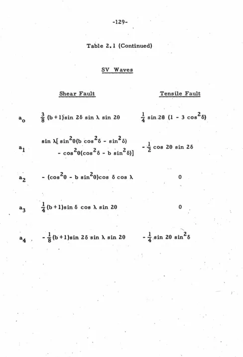
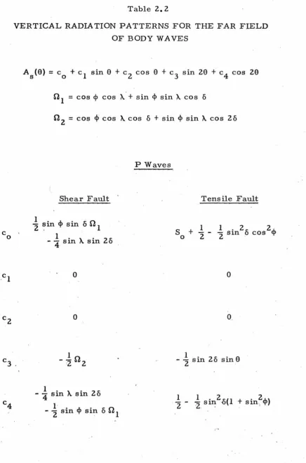
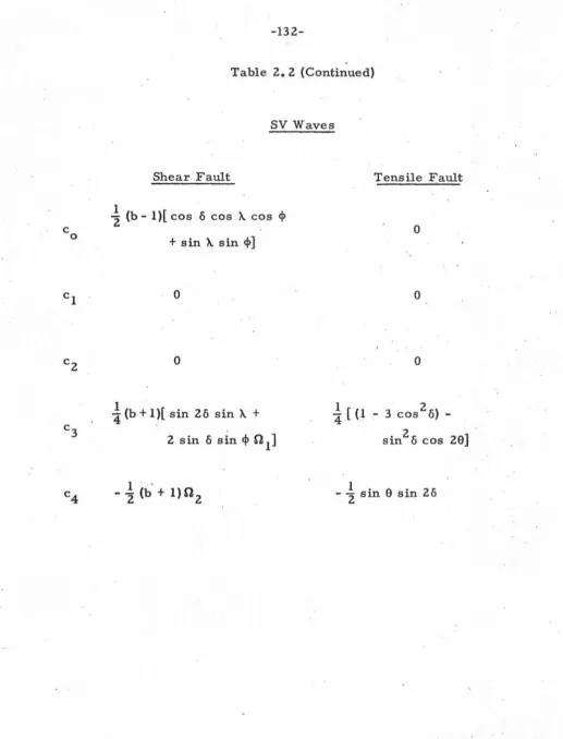
found to be useful and they are summarized in Tables 2.1 and 2.2,

in which we have defined the following parameters

b=

~(;~

-1)

=

s

=

(

1-

~~)

/(

1

+

;!z

1

1

=

0 3 - 4cr

cr being the Poisson's ratio. Notice that for a Poisson's solid,

where b

=

0

=

~

,

obtained in an earlier paper (Ben-Menahem, Smith, and Teng, 1965),

which also conform with the results obtained by Knopoff and Gilbert

(1960) for a slip dislocation with a continuous normal stress field.

2. 4. 3. Body Force Equivalents

It has been pointed out by Vvedenskaya (1956) that the

dis-~ placement field due to a displacement dislocation can be identically

reproduced in the absence of dislocation surface by a certain properly

chosen combination of body forces. Mathematically it means that

in (2. 30} and (2. 31) the vector fields

~

-

-

-generated by a distribution of F over S in the absence of Q can

-be reproduced by a proper choice of distribution of Q in V in the

absence of S. Studies along this line have been advanced by Knopoff

of the delta function, Burridge and Knope££ (1964) were able to obtain an explicit expression to calculate the equivalent body forces with a given dislocation. On ~he assumption .of continuity of normal stress

across the dislocation sheet, Burridge and Knope££ have shown that

-a displ-acement disloc-ation t-angenti-al to the disloc-ation sheet is

equivalent to a double couple body force with zero net moment, and

the one normal to the dislocation sheet is equivalent to a double force

with zero moment plus a pure dilatation. Similar results had been

obtained in an earlier paper (Knope££ and Gilbert, 1960}.

In this section we shall approach the problem in a different

way. We begin with assuming that in an infinite domain V free

-from dislocation surface, there exists a force density Q of an

uncle-termined strength £

0 in the following form

_ { iwt } _ _

Q

=

I

I)

We then compute the far displacement field due to a couple force

constructed from

Q

assign to £ so· that an identical radiation field as described by (2. 50)

0

to (2. 52) can be reproduced? It will be shown that the answer to this

question enables us to define the moment of a seismic source which

will iead easily to the calculation of the total seismic energy.

Using (2. 30) and (2. 31), we can write the displacement fields

-due to Q in (2. 64) in an infinite domain free from dislocation

-ik

I

r-; r'

I

.

u; (;)

=

~

H

H:z

e

1:

-:-:·

'

I

7Jr].

hL.l::.,.)}

1-;

I>;;]

F { · iwt }

=

~

+

po. .

-ik

17 I

e a

-

--(a• e ) e

r r {2. 65)

Similarly, we have

{2. 66)

- s _ F 0 { e iwt }

US H ( r )

=

f3

w-r..-)

where the superscript s denotes single force, and F = f dv is the

• 0 0

total force inside V. The displacement field due to a couple force

rrc is obtained by the application of a differential operator to rrs

such that

- c - - s

U

= -

where d is the spacing of the two opposite single force's. In the

' ' curvilinear coordinate system ( .;

1,

g

g

type can be express.ed by writing out the

g

--where d.

=

s are the metrical coeffic i'ents.

1 1 1

Clearly, the other components of the type of (2. 69) can be obtained by cyclic permt:':ations of the subscripts. By performing the

indicated operations, we. find the far field displacements due to a couple force

F d

- c - o

Up(r) =~ pa.

~ __.. -.. -. •e)(e •n)e ·

r r r (2. 70)

(2. 71)

(2. 72)

These fields cannot be made equal to those given in (2. 50) to (2. 5.2)\ whatever choice of f

0 is to be made. Study of (2. 70) to (2. 72) reveals that the only pos"sibility is to add the contributions from another couple force obtained from the field due to the single force

-*

{

.

Q

=

+ . )

.

1-; I )

~

0 1W .1WT (2. 73)

·

-by applying again the operator - d{ a •

\7),

c

'

-

-to be determined. B,.ecause of the symmetry existing in ·a and • n between the two· couple forces, the rad.iation patterns of the second

contributions which give

(2. 74)

{2. 75)

(2. 76)

In order to equalize the. fields in (2. 74) to (2. 76) to those in

J2. 50) to (2. 52), it is sufficient to require that

2 2C

=

132

(2. 77)

and

L ds

F d ₀

=

Comparing {2. 64) and {2. 73) in view of {2. 77) and (2. 78),

we conclude that, to reproduce the field generate

a

defined in {2. 40), it will be sufficient to superpose the fields p.

ro-duced by two perpendicular force couples with opposite but not

necessarily equal moments. ·One couple has the moment (L ds/21T)jJ.,

. 0

the other -{L ds /41T){X.

+

0 .

L ds

--=-0-

(~

-

~)

=

4'n'

L ds

0 40" - 1

~ Z(l - Z<T) (Z. 79)

the quantity inside the brackets approaches zero in the earth's crust where <T is around 0. 25, and becomes 1/4 in a depth of about 600 km where <T is about 0. 3. Therefore our model predicts a net moment which can be as large as a quarter of the dipole. moment. Many authors, e.g., Steketee (1958) and Keilis-Borok (1957), have pointed out that the direct P- and S-waves give information which

concerns with a non-equilibrium state, for the occurrence of an earthquake is essentially a break-down of static equilibrium. So far as the radiation of P- and S-waves is concerned. there is no a priori reason that it has to satisfy the condition of equilibrium at every instant ~uring the rupture process. · However, as soon as

the rupture process has ceased, and the P- and the S-wavefronts have left the· source region, equilib.rium in the source neighborhood must

l

be restored. F~rther, from the cons ide ration of conservation

.

.

. .

process if there is no external force acting on the source region. Therefore it is only plausible that a source model appropriate to the

. ~

initial motions does not have to be in equilibrium, but a complet~

source model explaining the entire seismic signals ought to be a statically balanced one. Recalling 'that we started in section (2 •. 4. Z) · with the sourc~ displacement (2.40) and ended up with the S-wave

radiation patterns (Z. 51) and (Z. 52) which, as checked by the results

(2. 75) and (2. 76) calculated from a double-couple source model, are

found to represent an unbalanced source. Therefore, it is concluded

that in order to construct a balanced source model, the displacement

(2.. 40) has· to be m.odified to a dislocation of Volterra type or one of Somigliana type (Steketee, 1958) so as to insure vanishing moment.

These results have' been obtained by various authors (e. g., Knopoff

and Gil~ert, 1960), which we shall not repeat here. However, we

have obtained the equivalent results from the body-force approach

(if setting C

=

=

and 2. 2) which, of course • is appropriate for a double-couple force of ·

vanishing moment. These results will be used in chapters 5 and

6.

2. 4. 4 Energy Calculation

-In the previous section .we have a:~rive·d at an. expression of. the moment for an equivalent force couple in terms· of sou~rce displace-ment L

0 ~nd area ds of a dislocation shE;:et • . By th~· theory ·of

body-wave amplitude equalization which we shall formulate in the

following section, the quantity L

o

.

.

terms of deformation work done upon the occ'urrence of the

dis-;

location.

Considering a fictitious force of magnitude F acting at the

0

source and causing a net displacement L

0 we define the energy I

emitted by a seismic source to be equal to the work done by

' .

F:

L

Energy

=

S

°

(2. 80)

Assuming that F

0 remains constant over the process of dis-. placement, we then have for a double-couple force

(2.81)

Notice that this is not the partial energy carried by the P- or 5-wave alone. It is the total energy of the seismic source, provided that the_presense of a free surface does not significantly change the .pcirtition of energy among P,· S, and other wave types. The quantity

inside the brackets of (2. 81) is directly ·measurable from the

body-. .

wave amplitude observed on the surface of the earth. The quantity

' .

Chapter 3

PROPAGATION OF BODY WAVES

The formal solution to the wave equation in an isotropic,

elastic, and spherical earth comes from the formulation of the

natural boundary value problem. Th~ result is generally expressed

by a triply infinite sum of zonal harmonics that reduce to a doubly

infinite sum when azimuthal independence of the source term is

assumed (Sate,~ al., 1963; Gilbert and MacDonald, 1960). Each

term of the series has an unambiguous physical interpretation in

terms of normal modes of the earth's free oscillation; while the

triple .sum is over surface wavelength, radial mode number, and

azimuthal mode degree. Since the earth is a finite body, its

eigen-values constitute a discrete set which becomes quite compact toward

the higher terms. Each discrete mode corresponds to a standing

wave pattern, and the interference of the standing waves gives rise

to the travelling waves which show on a conventional seismogram.

Further, it can be shown that th~ higher modes contribute mainly

to the body waves, while the lower modes are primarily responsible

to the surface waves (Sate~ al., 1963). It has been pointed out by

Brune (1964) that the energy in the lower modes, especially the

fundamental mode, is usually sufficiently separated from the

)

neighboring modes that each individual mode can be analyzed

separately. However, the energy. in the higher modes is always so

closely associated in ;requency and time that no part of the time

Mathematically, this is equivalent to the statement that the surface

I

waveform can usually be realized by one or a.few terms of the series

solution. Whereas the realization of a body-wave signal requires the

summation of a large numb.er of higher-order terms of the harmonic

series which makes the normal mode approach to the body wave

prob-lem very impractical, if not impossible. This difficulty does not

necessarily suggest that the physical mechanism of body-wave

propa-gation per se is more complex. Rather, it indicates that normal

mode expansion in terms of zonal harmonics is efficient only for a

\

long sinusoidal wave train such as the surface waves, but becomes

-quite inefficient for pulse-like bo,dy waves. There are ways to

over-come this difficulty (Bremmer, 1949; Ben- Menahem, 1964}. By

applying the Watson's transformation to the series solution followed

by taking the saddle-point approximation of the resulting complex

integral, it is possible to reach an approximate solution for the body

waves. The phase term of this approximate solution gives

expres-sions of the ray path and the travel time, while the amplitude term

gives the factor of geometric spreaqing. A study of the ray theory.

reveals that the above saddle-point solution, despite its laborious

mathematical derivations, provides hardly any more information than

that furnished by the simple ray method.

In the two following sections t~e ray theory will be expanded

and its limitations discussed. In the third section, we shall discuss

within the framework of the ray theory the attenuation of seismic

fails to satisfy the conditions of the ray theory, it will be

supple-mented with the more rigorous wave theory. Thus in regions like

the earth's crust or the core-mantle boundary where the variation

' I •

of seismic velocities is larie within one wavelength,

Thomson-Haskell's formulation will be used to account for the effec.ts 'Of

reflection and transmission across the layered boundaries, and

these will be presented in the fourth section. Inside the shadow

zone the observed body waves have gone through a diffracted path

along the core-mantle boundary. Wave phenomenon along this path

cannot be accounted for by the simple ray theory, we therefore have

to make use of the solution to the appropriate boundary value

prob-lem. We shall discuss this in the fifth section. In Appendix 3, we

shall derive some practical formulas suitable for the electronic

com-puter to calculate the integrals for travel time, ray path, attenuation

and the factor of geometrical spreading.

3.1. The Ray Theory as an Asymptotic Wave Theory

In the study of certain initial boundary value problems for

I

linear partial differential equations, an important class of asymptotic

methods is characterized by the fact that certain space curves,

known as "rays,'' play a fundamental role. All the functions that

make up the various terms of the asymptotic expansion can be shown

to obey some ordinary differential eq~ations along the rays. Often these equations can be solved immediately, yielding explicit

expres-.' sions for the asymptotic solution • . Th'is asy~ptotic method is useful

exact solution.

3 .1.1. Historical Remarks

The original idea of the ray approximation was formulated by

Sommerfeld and Runge (1911) following a suggestion from P. Debye.

In their argument a scalar function u, which in our case may

repre-sent the displacell}.ent field of a longitudinal or transverse wave

motion, is assumed to obey the scalar wave equation

2

2

\7u+ku.=0 (3.1)

where k is the wave number, representing either w/a. or w/r>.

Further,. the solution of (3.1) is assumed to have the form

-

·

_ ik

03 {?c)

u

=

where k

0 = w/c with c being phase velocity. Both A and g are

independent ~f the frequency. Direct substitution of (3. 2) into (3.1)

gives

-lk~u

[rvsl

2

-

:~]

+

Zik

u [

~

2

s

+

ln A) • \73]

0

ik g :

+

=

Dividing (3. 3) through by k2u and assuming that the resulting last

0 . .

. 2 2

term on the left-hand side, namely : \7 A/k

0A, remains small

as k

0 becomes infinite, we then find that it is sufficient to satisfy

and

(V' ln A) • · ('08)

+

l

2

(3. 4)

(3. 5)

(3. 4) is the well-known eikona1 equation, and its solution g

=

surfaces g= constant, or along a ray. With (3.4) and (3.5), most of the results in geometrical optics can be derived. For several decades, Sommerfeld and Runge's formulation of the ray theory had received much attention. Unfortunately, a number of ad hoc assumptions involved make their derivations not completely satis-factory. First, the derivation from the scalar wave equation is not sufficiently general. Secondly, the solution (3. 2) represents a very restricted class of field. That A is assumed to be freque

ncy-independent is only fulfilled for plane waves in a homogeneous medium. Thirdly, the g and the A, which constitute the solution to (3 .1)

through (3.2), are obtained from (3.4) and (3.3) at the limit when k 0

is infinite. This is not quite proper because the solution (3. 2) con-ik g

tains the factor e 0 which has no limit as k becomes infinite.

0

A desirable derivation should not only be free from the above objections but also be· able to offer insight into the connection between

.I

transition from one to the other. 3 .1. 2. Asymptotic Ray Theory

Recently, a class of more general ray theories have been

extensively developed primarily by J. B. Keller and his colleagues

at Courant Institute. A number of papers (in particular, Karal and Keller, 1959; Keller and Karal, 1960, 1963), have offered special interest to the elastic wave propagation in both homogeneous and inhomogeneous media. Following the discussion of Karal and Keller (1959), we may write the equation of motion

-

-+

v._..

We now seek a time harmonic solution of the form -_{U =Ae} - iw(o - t)

et (3. 7)

-

-where A and g are functions of x • Substituting (3. 7) into (3. 6) and cancelling the exponential factor, we obtain

2 - -

-- (iw) pA + (X. + ._.,)(iw'Vg + 'V)('V • A + iwA • Vg)

2- - 2- 2 - 2

+ ._.,[

\1

_., -. _,.. --..

In obtaining (3. 8), the following vector identities are used

\l •

U

We now assume that g is independent of frequency. To establish

the connection between the geometrical ray theory· and the more

-general wave theory, we assume that A possesses an expansion as

inverse powers of frequency

-

~-

A

=

·

L

n=O

-

-The vectors A to be determined are functions of x only. Series n

expansion of the type (3. 9) is suitable for high frequencies. However,

experience has shown that it is still useful at frequencies so low

that the wavelength is comparable to other dimensions of the

prob-lem. Putting (3. 9) into (3. 8), we obtain

(X)

\ (iw)-n[ -(iw)2pA +(A.+ fJ.}{iwVS+ V)(V • A + iwA • \J3)

L

n=O

+ \l A. { iw( A • \l S) + (V • A ) } + (VA.) X { iw (V g X A ) + \l X A ) }

n n n n

Since (3 .10) does not just hold for a fixed frequency 1 the coefficient

of each term in the power expansion must vanish. Therefore 1 we

have for n

=

(3 .11) Taking the dot product of (3 .11) with \7~₁ it yields

(3.12)

The cross product of 'VS with (3.11) gives

-

-

-Since neither A nor 'V~ is identically zero 1 A • 'VS and A X 'VS

0 0 0

cannot be zero simultaneously.. Likewise the two expressions inside the brackets in (3.12) and (3.13) cannot vanish at the same time. Therefore, (3.12) and (3.13) resolve into two sets of simultaneous equations

-I

. 0

('VS)2

=

~

(3 .14) (3 .15) a

and

-

0 (3.16)

The first set describes a wavefront propagating at· the longitudinal

-wave velocity a, having the displacement A normal to the wave-o

front surface. The second set describing a wavefront propagating at

-the transverse wave velocity

13,

tan-o

gential to the wavefront surface. When the medium is homogeneous,

the wavefront from a point source forms a family of concentric

spheres, and the rays are straight lines. In an inhomogeneous

medium, the wavefront is no longer spherical, and the rays are

curvilinear curves. These properties of rays and wavefronts will

be discussed in more detail in the next section.

Now, again from {3.10) we have for n = 1

-

-+

+

=

0 0 (3.18)

-{3 .14), -{3 .15), and {3 .18) lead to an equation of A

0 for the

longitudin~l ~ave. On the other hand, {3.16), {3.17), and {3.18) lead to an equation of

A

0

We shall first treat the ca.se of the longitudinal wave. The last term of {3.18) vanishes by virtue of {3.14), which also.'implies that

-

=

VS

where a

0 is a scalar proportionality factor. Dotting the remaining

equation (3.18) by \7g, it is easy to show by use of (3.15) and (3.19)

that (3.18) reduces to the following simple form

2(\?S • \?}a

+

.!.

=

0 p 0 ' (3. 20}

Since S is known from (3 .15} _, therefore (3. 20} is an equation

-for a which, in light of (3 .19}, yields A in question. Now,

0 . 0

since \7S is a vector normal to the wavefront or tangential to the

ray, so \7S • \7 is simply an operator of directional differentiation

along a ray. Again (3.15) implies ·

IVS I

we

may

where a is the arclength along the ray. Introducing (3. 22) into (3. 20),

the equation of a

0 can be written in the form

dao

.!. [.!.

ds

+

This equation describes the amplitude behavior along the ray path.

An integration along the ray path between a

(3. 24)

·To compute the remaining integral, we consider a tube of rays

ter-· minating in both ends by ~l and ~

2

g = t

1 and

S

2 being arbitrary constants. Let ~

3

2

Hence ~l, ~

2

3

divergence theorem to the function \728

-\78 • d<r

v

-where d CT is the outward normal. Since

'VS

ray_, we have, in light of (3. 21)

-

I'Vsl

dcr 1

\78 • d CT

= -

= -

-

2

'Vg •

=

I

=

ars::T

a s 2

-'VS •

=

S

j'

S

V

=

S S

~J

v :Ez

·(3.26)

Next we choose an arbitrary wavefront which intersects the tube of

rays to form a surface I;. By expressing that

(3. 27)

where dcr are surface element-s of :E; K

1 and K2 are proportional

constants measuring the expansion of an infinitismally narrow tube

of ray, we may then write (3. 26) as

=SS

1::

\sz.

~-

(K)

j

1

The volwne element dv can .be written as

dv

=

Since V is arbitrary, we must have

V'2g

=

K)

K da a

Note that this result (3. 28) is similar to the one obtained by Luneberg (1944) in the case of geometrical optics. Introducing (3.28) into (3. 24) and noting that

.2...

(K)

we obtain with the aid of (3. 27)

(3.28)

(3.29)

In view of (3.19), we finally arrive at the expression of ge~metrical

i

IA

I

IA

I

(3. 30)

Here dcr(s

1) and dcr(s 2)· denote cross-sectional area of a tube of

rays at

a

1 and

a

is the limit