This is a repository copy of
Game Theoretic Decentralized Feedback Controls in Markov
Jump Processes
.
White Rose Research Online URL for this paper:
http://eprints.whiterose.ac.uk/113170/
Version: Accepted Version
Article:
Bagagiolo, F., Bauso, D. orcid.org/0000-0001-9713-677X, Maggistro, R. et al. (1 more
author) (2017) Game Theoretic Decentralized Feedback Controls in Markov Jump
Processes. Journal of Optimization Theory and Applications. pp. 1-23. ISSN 0022-3239
https://doi.org/10.1007/s10957-017-1078-3
The final publication is available at Springer via
http://dx.doi.org/10.1007/s10957-017-1078-3
[email protected] https://eprints.whiterose.ac.uk/ Reuse
Unless indicated otherwise, fulltext items are protected by copyright with all rights reserved. The copyright exception in section 29 of the Copyright, Designs and Patents Act 1988 allows the making of a single copy solely for the purpose of non-commercial research or private study within the limits of fair dealing. The publisher or other rights-holder may allow further reproduction and re-use of this version - refer to the White Rose Research Online record for this item. Where records identify the publisher as the copyright holder, users can verify any specific terms of use on the publisher’s website.
Takedown
If you consider content in White Rose Research Online to be in breach of UK law, please notify us by
(will be inserted by the editor)
Game Theoretic Decentralized Feedback Controls in
Markov Jump Processes
Using the LaTex Template
Fabio Bagagiolo · Dario Bauso · Rosario Maggistro · Marta Zoppello
Received: date / Accepted: date
Fabio Bagagiolo
University of Trento
Trento, Italy
Dario Bauso
University of Sheffield
Sheffield, England
Rosario Maggistro (corresponding author)
University of Trento
Trento, Italy
Marta Zoppello
University of Trento
Trento, Italy
Abstract This paper studies a decentralized routing problem over a network, using the paradigm of mean-field games with large number of players. Building
on a state space extension technique, we turn the problem into an optimal
con-trol one for each single player. The main contribution is an explicit expression
of the optimal decentralized control which guarantees the convergence both
to local and global equilibrium points. Furthermore, we study the stability of
the system also in the presence of a delay which we model using an hysteresis
operator. As a result of the hysteresis, we prove existence of multiple
equilib-rium points and analyze convergence conditions. The stability of the system
is illustrated via numerical studies .
Keywords Optimal control· Mean field games ·Inverse control problem ·
Decentralized routing policies· Hysteresis
Mathematics Subject Classification (2000) 91A13 · 91A25 · 49N25·
49L20·47J40
1 Introduction
In recent years, dynamics on networks have sparked interest in different
ap-plication domains such as data transmission, traffic flows and consensus (see
[1–3]) just to name a few. In this paper, we investigate a routing problem
defined over a network. The problem involves a population of individuals,
re-ferred to as players. As main contribution, we provide convergence conditions
to an equilibrium point, characterized by uniform distribution over all the
given the observed distribution of the other players. To prove such a
conver-gence result, we recast the problem within the framework of optimal control
theory. A similar problem is studied in [4], in which the authors consider a
centralized control and a density flow for each edge dependent on the density
of the whole population. This implies that each player minimizes a common
cost functional which depends on the whole population’s density distribution.
Differently from [4], we consider a decentralized control (as in [5–7]), in which
the density of each node is controlled locally. We highlight next three distinct
approaches relating to routing/jump problems. The first one consists in
con-trolling the probability to jump from a node to another one (or to flow along
the edges) [4]. The second one consists in controlling the transition rate from
nodes (or edges) [8], and the last one in assigning the product among the
probability and the relative transition rate. As in [9], in this paper we use the
last approach, in particular we control the product between the probability
to jump from one node to an adjacent one and the relative transition rate.
In the same spirit as in inverse control problems, [10], we provide an explicit
expression of the running cost function in order to obtain our desired optimal
feedback control as solution of the optimal control problem.
In this paper, we consider the problem of stabilizing the system under the
assumption that each agent ignores both the controls of the far agents and the
network topology. We formulate the problem as follows: from a microscopic
point of view, each player jumps from a node to an adjacent one according to a
is characterized by a dynamics describing the time-evolution of the density.
Such dynamics depends on a decentralized control. We rearrange the problem
as a mean-field game and then via a state-space extension approach as an
optimal control one. The state space extension procedure is reminiscent of the
McKaVlasov control problem, in which the statistical distribution is
en-coded by our density. Similarities and differences between the McKean-Vlasov
and the Mean-Field framework are analyzed in [11].
Furthermore, we prove convergence to a local equilibrium which is
character-ized by an equal density on the neighbor nodes. Finally, we prove a similar
con-vergence result for the global equilibrium, characterized by a uniform
distribu-tion of the density over all nodes. We then introduce a hysteresis operator
act-ing on the optimal feedback decentralized control. A similar model was already
discussed in [12]. The authors make a rigorous treatment of continuous-time
average consensus dynamics with uniform quantization in communications.
The consensus is reached by quantized measurement which are transmitted
using a delay thermostat. In contrast to this, we use a different hysteresis
op-erator, the play opop-erator, that can be considered as a concatenation of delayed
thermostats. Moreover, we apply such an operator to our control, and this
re-sults in a nonlinear dynamics. We use an hysteresis to capture a scenario where
the players have distorted information on the density distribution in neighbor
nodes. We prove that the problem has multiple equilibrium points, and we
1.1 Related Literature
The mean-field game theory was developed in the work of M.Huang, R. Malham´e
and P. Caines [13, 14] and independently in that of J. M. Lasry and P.L.
Li-ons [15,16], where the new standard terminology of Mean Field Games (MFG)
was introduced. This theory includes methods and techniques to study
differ-ential games with a large population of rational players, and it is based on the
assumption that the population influences the individuals’ strategies through
mean-field parameters. In addition to this theory, the notion of Oblivious
Equi-libria for large population dynamical game was introduced by G. Weintraub, C.
Benkard, and B. Van Roy [17] in the framework of Markov Decision Processes.
Several application domains, such as economic, physics, biology and network
engineering accommodate mean-field game theoretical models (see [16,18–20]).
Decision problems with mean-field coupling terms have also been formalized
and studied in [21], and application to power grid management are recently
provided in [22]. The literature provides explicit solutions in the case of linear
quadratic structure. In most cases, a variety of solution schemes have been
recently proposed, based on discretization and or numerical approximations
(see [18, 23]). Computing an explicit solution in the nonlinear case is difficult,
and therefore in this paper, in spirit with [24, 25], we reformulate the problem
as an inverse optimal control problem.
Regarding hysteresis, the concept of hysteretic operator is due to Krasnoselskii
and his co-worker [26]. There are several physical and natural phenomena in
tran-sition, superconductivity, shape memory and communication delay (see [12,27]
for more details).
1.2 Structure of the Paper
This paper is organized as follows: a mean-field game formulation of the
prob-lem is provided in Sect. 2. In Sect. 3, we introduce a state-space extension
solution approach which is an alternative method to the classical fixed point
one and exhibits the optimal decentralized feedback control under a suitable
assumption. In Sect. 4 we study the convergence to and the stability of a local
Wardrop equilibrium and then its extension to a global equilibrium. In Sect. 5
we carry out numerical studies. Finally, in Sect. 6 we introduce the play
oper-ator which acts on the control function, and study both the global equilibrium
and the stability of the density equation subject to this operator.
2 Model and Problem Set-up
In this section, we provide a model of a pedestrian density flow over a network
with dynamics defined on each node, and using a line graph as topology. Let
G be a graph with h nodes, e edges, and vertex degree di for i = 1, . . . , h. We define the line graph L(G) = (V, E) to be the graph with n = e nodes andm= 1
2
Ph
i=1d2i edges. In particular, the graph is obtained by associating a vertex to each edge of the original graph and connecting two vertices with
jumps between vertices. Now, let a connected line graph L(G) = (V, E) be given, where V ={1, . . . , n} is the set of vertices andE ={1, . . . , m} is the set of edges. For each node i∈V, let us denote by N(i) the set of neighbor nodes ofi:
N(i) ={j∈V :{i, j} ∈E}.
We consider a large population of players and each of them is characterized
by a time-varying state X(t)∈V at timet ∈[0, T], where [0, T] is the time horizon window. Players represent pedestrians and jump across the nodes of
the graph according to a decentralized routing policy described by the
matrix-valued function
u(·) :R+−→R+n×n, t7−→u(t). (1)
Note that utakes value in Rn+×n because each component uij is the product between the probability to jump from one node to an adjacent one and the
relative transition rate.
Leti∈V be the player’s initial state. The state evolution of a single player is then captured by the following continuous-time Markov process:
{X(t), t≥0}
qij(uij) =
uij, j∈N(i), j6=i,
−Pk∈N(i),k6=iuik, i=j,
0, otherwise,
whereqij is the microscopic dynamics fromito j.
Denote by ρthe vector whose components are the densities on vertices. This implies that the sum of the components is equal to one. Thus we have
ρ∈D:={ρˆ∈[0,1]n :X i∈V
ˆ
ρi= 1}.
The density evolution can be described by the following forward Kolmogorov
Ordinary Differential Equation (ODE)
˙
ρ(t) =ρ(t)A(u), ρ(0) =ρ0,
(3)
where ρ is a row vector, ρ0 is the initial condition and the matrix-valued
functionA:Rn+×n→Rn×n is given by
Aij(u) =
uij ifj ∈N(i), j6=i,
−Pj∈N(i),j6=iuij ifi=j,
0 ifj 6∈N(i).
Equation (3) establishes that the density variation on each node balancing
densities on neighbor nodes.
It is well known that the uniform distribution of the density on a graph
corre-sponds to a Wardrop equilibrium [28]. Since we are considering a line graph,
our aim is to achieve a uniform distribution of the density over all nodes. Indeed
in traffic network the Wardrop equilibrium corresponds to equidistribution of
agents along edges. Therefore on its line graph we view the equilibrium as
equilibrium, i.e. a uniform density on the nodes adjacent toi. For each player, consider a running cost ℓ(·) :V ×[0,1]n×Rn×n
+ →[0,+∞[,
and an exit costg(·) :V ×[0,1]n→[0,+∞[ of the form given below
ℓ(i, ρ, u) = X j∈N(i),j6=i
u2ij
2 (γij(ρ))
+
, (4)
g(i, ρ) =dist(ρ,Mˆi). (5) where γij is a suitable coefficient yet to be designed and (·)+ is the positive part operator.
In (5) thedist(ρ,Mˆi) denotes the distance of the vectorρfrom the manifold ˆ
Mi, where ˆMi is the local consensus manifold/local Wardrop equilibrium set for the playeridefined as
ˆ
Mi={ξ∈Rn:ξj=ξi ∀j∈N(i)}. (6)
Therefore, the choice of the exit cost g(i, ρ) describes the difference between the number of agents in the node i and the local equidistribution of agents among the adjacent nodes.
The problem in its general form is then the following:
Problem 1: Design a decentralized routing policy to minimize the output
dis-agreement, i.e., each player solves the following problem:
infu(·)J(i, u(·), ρ[·](·),·),
J(·) =RtTℓ(X(τ), ρ(τ), u(τ))dτ+g(X(T), ρ(T)), {X(t), t≥0} as in (2),
X(t) =i,
whereuis the control (1) taking value inRn+×nfor anyt∈[0, T] andρevolves
as in (3). Note that every player minimizes a cost functional which depends
on the density of his neighbours. Thus, the microscopic (2) and macroscopic
(3) representations of the system are strongly intertwined which makes the
problem different from classical optimal control.
2.1 Mean-Field Formulation
This subsection presents a mean-field formulation of problem (7). Let v(i, t) be the value function of the optimization problem (7) starting from timet in statei. We can establish the following preliminary result.
Lemma 2.1 The mean-field system for the decentralized routing problem in Problem 1 takes the form:
˙
v(i, t) +H(i, ∆(v), t) = 0in V ×[0, T[, v(i, T) =g(i, ρ(T)),∀x∈V,
˙
ρ(t) =ρ(t)A(u∗), ρ(0) =ρ0,
(8)
where
H(i, ∆(v), t) = inf u
X
j∈N(i)
qij(v(j, t)−v(i, t)) +ℓ(i, ρ, u)
, (9)
andg is given as in (5).
optimal time-varying control u∗(i, t)is given by
u∗(i, t)∈arg min u
X
j∈V
qij(v(j, t)−v(i, t)) +ℓ(i, ρ, u)
. (10)
Proof.:To prove the first equation of (8) we know from dynamic programming
that
˙
v(i, t) + inf u
X
j∈N(i)
qij(v(j, t)−v(i, t)) +ℓ(i, ρ, u) = 0 inV ×[0, T[.
We obtain the first equation, by introducing the Hamiltonian in (9). Since
(2) depends on the routing policy u, then the latter is obtained minimizing the Hamiltonian as expressed by (10). The second equation is the boundary
condition on the terminal cost. The third and fourth equation are the forward
Kolmogorov equation and the corresponding initial condition. ⊓⊔
The mean-field game (8) appears in the form of two coupled ODEs linked
in a forward-backward way. The first equation in (8) is the
Hamilton-Jacobi-Bellman (HJB) equation with variablev(i, t) and parametrized inρ(·). Given the boundary condition on final state and assuming a given population density
behaviour captured byρ(·), the HJB equation is solved backwards and returns the value function and the optimal control (10). The Kolmogorov equation is
defined on variableρ(·) and parametrized inu∗(i, t). Given the initial condition
ρ(0) = ρ0 and assuming a given individual behaviour described by u∗, the
density equation is solved forward and returns the population time evolution
3 State Space Extension
We solve Problem 1 and the related mean-field game (8) through state space
extension, in spirit with [4]; namely we reviewρas an additional state variable. Then the resulting problem is of the form
inf
u(·) J(i, u(·), ρ[·](·),·),
subject to {X(t), t≤0} as in (2),
˙
ρ(t) =ρ(t)A(u).
We are looking for a value function ˜V(i, ρ, t) which depends oniand on the density vectorρas a state variable, rather than as a parameter as in (7). The problem can be rewritten as follow.
Lemma 3.1 The mean-field system for the decentralized routing problem in Problem 1 takes the form:
∂tV˜(i, ρ, t) + ˜H(i, ρ, ∆( ˜V), ∂ρV , t˜ ) = 0 inV ×[0,1]n×[0, T[, ˜
V(i, ρ, T) =g(i, ρ(T)),
(11)
where for the Hamiltonian we have
˜
H(i, ρ, ∆( ˜V), ∂ρV , t˜ ) = inf u
X
j∈N(i)
qij( ˜V(j, ρ, t)−V˜(i, ρ, t))+∂ρV˜(i, ρ, t)(ρA(u))T+ℓ(i, ρ, u)
,
(12)
and the optimal time-varying controlu∗(i, ρ, t)is given by
u∗(i, ρ, t)∈arg min u
X
j∈N(i)
qij( ˜V(j, ρ, t)−V˜(i, ρ, t))+∂ρV˜(i, ρ, t)(ρA(u))T+ℓ(i, ρ, u)
.
Proof:From dynamic programming we obtain
∂tV˜(i, ρ, t)+inf u
X
j∈V
qij( ˜V(j, ρ, t)−V˜(i, ρ, t))+∂ρV˜(i, ρ, t)(ρA(u))T+ℓ(i, ρ, u)
= 0.
By introducing the Hamiltonian ˜H(i, ρ, ∆( ˜V), ∂ρV , t˜ ) given in (12), the first equation is proven. To prove (13), observe that the optimal control is the
minimizer in the computation of the extended Hamiltonian. Finally, the second
equation in (11) is the boundary condition. ⊓⊔
Remark 3.1 The use of the state space extension approach reduces our initial problem to an optimal control problem. Therefore from now on we will no
longer consider the mean field formulation.
Now, our aim is to review the optimal control problem as an inverse problem.
Our aim is to find a suitable γij (see (4)) such that the optimal control u∗ij, which is theargminof the extended Hamiltonian, is
u∗ij =
ρi(t)−ρj(t) ρi(t)> ρj(t), j∈N(i),
0 otherwise.
(14)
In [4] for the infinite horizon problem, the authors take the value functions
asV(ρ) =dist(ρ, M), whereM is the global equilibrium manifold. Therefore in our finite horizon problem we assume that
V(i, ρ) =dist(ρ, Mi) =
v u u u
t X
j∈N(i) ρj−
P
k∈N(i) ρk #N(i)
!2
. (15)
Note that the above satisfies the boundary condition in (11), according to our
choice of the exit costg (see (5)).
˙
ρi(t) =
X
j∈N(i),j6=i
ρj(t)uji−
X
j∈N(i),j6=i
ρi(t)uij.
Starting from the Hamiltonian (12) (see also (4)) we assume that if ρi 6=ρj,
γij is
γij(ρ) =
ρ2i −ρiρj−dist(ρ,Mˆj)dist(ρ,Mˆi) +dist(ρ,Mˆi)2 (ρi−ρj)dist(ρ,Mˆi)
!
. (16)
We want to prove that, using (16), the correspondent running cost (4) is such
that our control (14) is the optimal one. We have the following cases:
a) γij >0
The Hamiltonian (12) is strictly convex inuij. Therefore the optimal con-trol uij is the solution of
∂H˜ ∂uij
=uijγij(ρ) +
ρiρj−ρ2i
dist(ρ,Mˆi)
+dist(ρ,Mˆj)−dist(ρ,Mˆi) = 0. (17)
Namely ifρi> ρj,uij =ρi−ρj, instead ifρi< ρj since we are supposing that uij ∈R+ we have that the optimal control isuij = 0.
b) γij ≤0
The Hamiltonian (12) is linear in uij and is increasing or decreasing de-pending on the sign of
βij =
ρiρj−ρ2i
dist(ρ,Mˆi)
+dist(ρ,Mˆj)−dist(ρ,Mˆi) =−γij(ρ)(ρi−ρj)
– ifρi> ρjthe Hamiltonian is increasing inuij, hence it admits minimum atuij= 0 ,
Now note that, if the densities are converging in time to the same value,
which is the case if we use the controlu∗
ij, the function (16) is never
neg-ative and thus case b) before cannot occur. Simulations will show this
phenomenon and also suggest that
lim
ρi→ρj,j∈N(i)\{i}γij= +∞. (18)
which is coherent with the constraintu∗ij = 0. Therefore, using function (16), the corresponding running cost given by
ℓ(i, ρ, u) = X j∈N(i), j6=i ρi>ρj
u2ij
2
ρ2
i −ρiρj−dist(ρ,Mˆj)dist(ρ,Mˆi) +dist(ρ,Mˆi)2 (ρi−ρj)dist(ρ,Mˆi)
!+
| {z }
γij(ρ)
,
(19)
leads the optimal feedback control to take the same value as in (14). Moreover,
when using control (14), the Hamiltonian (12) also converges to zero asttends to infinity. Hence, the functionV(i, ρ) as defined in (15), is almost a solution of the Hamilton-Jacobi-Bellman problem (11). Such a consideration leads to
the fact that, at least when time becomes large, the control (14) is optimal.
The fact that the Hamiltonian (12) converges to zero derives from (17) where
the second addendum of the right-hand side is bounded (the distance from
the manifold is larger than |ρi −ρj| up to a multiplicative constant). This boundedness leads to (ρi−ρj)2γij(ρ)→0 and hence the conclusion, because inside the Hamiltonian we almost have (17) multiplied by (ρi−ρj).
Now with the control (14), we can rewrite the evolution ofρas ˙
ρi(t) =
X
j6=i,j∈N(i):ρj>ρi
ρj(t)(ρj(t)−ρi(t))−
X
j∈N(i):ρi>ρj
Now our aim is to study the stability properties of dynamical system (20).
In other words if using the optimal control u∗
ij the system converges to an
equilibrium.
4 Wardrop Equilibrium
In this section, we will show how to obtain a uniform distribution of the density
ρ, at first on a neighborhood of a node and then throughout the graph. The right-hand side of equation (20) is zero only when ρi =ρj ∀i ∈ V and
j∈N(i), which leads to a uniform density over the nodes.
The following assumption establishes that for a given feasible target manifold,
there always exists a decentralized routing policyu(t) which drives the density
ρtoward the relative manifold ˆMi (see (6)).
This assumption will be used later on to prove the convergence to a local
Wardop equilibrium.
[image:17.595.181.317.483.586.2]Assumption 1 (Attainability condition)
Let ˆMibe given by (6),r >0 andSi ={ρ:dist(ρ,Mˆi)< r}. For allρ∈Si\Mˆi there exists an element in the projection,ξ(i, ρ)∈ΠMiˆ ρ, such that the value val[λi] is negative for every λi = (ρ(t)−ξ(i, ρ)), namely
∀i, val[λi] = inf
u {λi·[(I−∂ρ(ξ(i, ρ))) ˙ρ
T+ X
j∈N(i)
(ξ(j, ρ)−ξ(i, ρ))qij]}<0, (21)
where∂ρξ(i, ρ) is a constant matrix sinceξ(i, ρ) is a linear function ofρ. We point out that, as we will show in Section 5 (see (25)), assumption (21) is
satisfied by our optimal controlu∗
ij (14).
Assumption (21) represents the trend of the agents in nodeito be influenced by the choices of the neighbor agents. Agents can act in order to reach the
same density as in the adjacent nodes.
In the proof of the next theorem, we review the value function of (11) as a
Lyapunov function.
Theorem 4.1 Let Assumption 1 hold true. Then, ρ(t)converges asymptoti-cally to Mˆi, i.e.
lim t→∞dist(ρ,
ˆ
Mi) = 0. (22)
Proof :Letρbe a solution of (3) with initial value ρ(0)∈Si\Mˆi.
Setτ={inft >0 :ρ(t)∈Mˆi} ≤ ∞and letV(i(t), ρ(t)) =dist(ρ(t),Mˆi). For allt∈[0, τ] andξ∈ΠMiˆ (ρ(t)). We wish to compute ˙V(i(t), ρ(t)) as the limit
the Markov process giving the evolution of the indexi(t), that is:
V(i(t), ρ(t+dt))−V(i(t), ρ(t)) +V(i(t+dt), ρ(t))−V(i(t), ρ(t)) =
kρ(t+dt)−ξ(ρ(t+dt), X(t))k − kρ(t)−ξ(ρ(t), X(t))k+
kρ(t)−ξ(ρ(t), X(t+dt))k − kρ(t)−ξ(ρ(t), X(t))k=
kρ(t) + ˙ρ(t)dt−ξ(ρ(t), X(t))− ∇ρξ(ρ(t), X(t)) ˙ρ(t)dtk−
kρ(t)−ξ(ρ(t), X(t))k+|dt|ε(dt)+
kρ(t)−ξ(ρ(t), X(t))−∂Xξ(ρ(t), X(t)) ˙X(t)dt+o(dt)k − kρ(t)−ξ(ρ(t), X(t))k
˙
V(i(t), ρ(t)) = lim
dt→0
1
dt
kρ(t) + ˙ρ(t)dt−ξ(ρ(t), X(t))− ∇ρξ(ρ(t), X(t)) ˙ρ(t)dtk2
kρ(t) + ˙ρ(t)dt−ξ(ρ(t), X(t))− ∇ρξ(ρ(t), X(t)) ˙ρ(t)dtk−
kρ(t)−ξ(ρ(t), X(t))k2
kρ(t)−ξ(ρ(t), X(t))k +|dt|ε(dt)+
kρ(t)−ξ(ρ(t), X(t))−∂Xξ(ρ(t), X(t)) ˙X(t)dtk2
kρ(t)−ξ(ρ(t), X(t))−∂Xξ(ρ(t), X(t)) ˙X(t)dtk
−
kρ(t)−ξ(ρ(t), X(t))k2
kρ(t)−ξ(ρ(t), X(t))k +o(dt)
= lim dt→0 1 dt
kρ(t) + ˙ρ(t)dt−ξ(ρ(t), X(t))− ∇ρξ(ρ(t), X(t)) ˙ρ(t)dtk2
kρ(t)−ξ(ρ(t), X(t))k+O(√dt) −
kρ(t)−ξ(ρ(t), X(t))k2
kρ(t)−ξ(ρ(t), X(t))k +|dt|ε(dt)+ kρ(t)−ξ(X(t))−∂Xξ(ρ(t), X(t)) ˙X(t)dtk2
kρ(t)−ξ(ρ(t), X(t))k+O(√dt) −
kρ(t)−ξ(ρ(t), X(t))k2
kρ(t)−ξ(ρ(t), X(t))k +o(dt)
=
1
kρ(t)−ξ(ρ(t), X(t))k d dt
kρ(t)−ξ(ρ(t), X(t))k2
≤
2
kρ(t)−ξ(i, ρ)k
(ρ(t)−ξ(i, ρ))·
(I− ∇ρ(ξ(i, ρ))) ˙ρ(t)T +
X
j∈N(i)
(ξ(j, ρ)−ξ(i, ρ))qij
.
Using now Assumption 1 we have that the second factor of the last product is
strictly negative, hence ˙V(i(t), ρ(t))<0. This proves not only that a Wardrop equilibrium but also that the solutionρof the dynamics (3) is locally
asymp-totically stable for the Lyapunov theorem. ⊓⊔
The next step is to prove the asymptotic convergence ofρ, solution of (3), to the global consensus manifoldM defined as follows
M ={ρ∈D:ρ=11
wherenis the number of nodes.
Corollary 4.1 Let Assumption 1 hold true, then
lim
t→+∞d(ρ(t), M) = 0.
Proof:We are in the hypothesis of Theorem (4.1), then
lim t→∞dist(ρ,
ˆ
Mi) = 0.
It follows that for any sequence (tm)m∈Nsuch thattm→+∞we have that
ρi →β
ρj →β ∀ j∈N(i)
ρk →β ∀ k∈N(j) s.tj∈N(i) ..
.
(24)
By doing this, since the graph is connected, we can conclude that
ρi(tm)→β = 1
n ∀i∈V.
Then, there exists a subsequence (tmℓ)ℓ∈Nsuch that
ρi(tmℓ)→ 1
n ∀i∈V.
5 Numerical Example
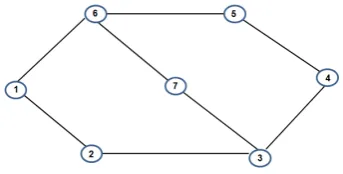
In this section, numerical simulation show that on a graph with seven nodes,
the provided distributed routing policy (14) provides convergence to the
equi-librium.
Consider the following network consisting of 7 nodes and 8 edges.
Fig. 2 Network system with seven nodes.
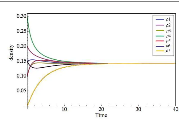
Solving the Kolmogorov equation (20) with the following initial conditions
ρ1(0) = 0.15, ρ2(0) = 0.2, ρ3(0) = 0.1, ρ4(0) = 0.3, ρ5(0) = 0.1, ρ6(0) = 0.15, ρ7(0) = 0,
[image:22.595.154.326.256.343.2]Fig. 3 Simulation of the density.
As expected the density converges to the global equilibrium in which all
theρi are equal.
In Fig. 4 we can see that the functionγij (16) is positive, in accordance with our statements in Section 3.
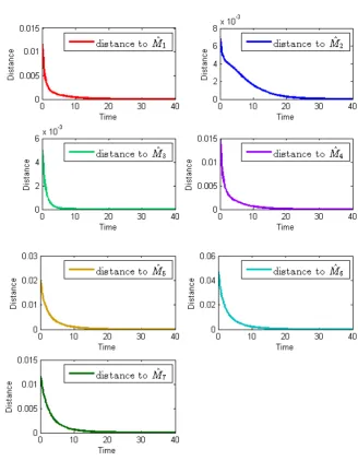
[image:23.595.77.378.78.285.2] [image:23.595.76.391.516.612.2]Note that the optimal control u∗
ij = (ρi−ρj)+ satisfies Assumption 1 as by defining
αi=λi·[(I−∂ρ(ξ(i, ρ))) ˙ρ(t)T +
X
j∈N(i)
(ξ(j, ρ)−ξ(i, ρ))qij], ∀i= 1,· · ·,7,
we have that the maximum values ofαi are
max
ρ {α1}=−6.1489·10
−7 max
ρ {α2}=−2.1462·10
−6
max
ρ {α3}=−3.1123·10
−9 max
ρ {α4}=−6.7065·10
−7
max
ρ {α5}=−8.0771·10
−7 max
ρ {α6}=−2.1169·10
−6
max
ρ {α7}=−7.4670·10
−7 .
(25)
Then, functionαi is negative for alli, for our choice of the control.
6 Stability with Hysteresis
In the following section we study stability of the macroscopic dynamics of the
vector ρwhen the optimal decentralized feedback control (14) is affected by a hysteresis phenomena modeled by a scalar play operator. We study how
the evolution of the macroscopic equation changes when we apply the play
operator to the controlu∗ obtained from (14). Furthermore, we characterize the set of equilibrium points as union of several manifolds. Finally, we provide
convergence condition for the resulting dynamics.
After introducing the play operator the controlled dynamical system is given
by ˙
ρ(t) =ρ(t)A(w), w(t) =P[u∗]+(t), ρ(0) =ρ0, w(0) =w0,
(26)
6.1 The Play operator
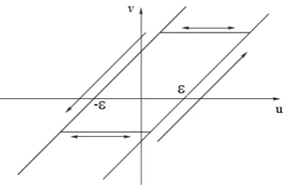
Fig. 6 Hysteresis play operator
Letε >0 be a parameter which characterizes the Play operator and define
Ωε:=
(u, v)∈R2:u−ε < v < u+ε .
The behavior of the scalar play operator v(·) :=P[u](·), with its typical hys-teresis loops, can be described using Fig. 6. For instance, supposing thatuis piecewise monotone, if (u(t), v(t))∈Ωε thenv is constant in a neighborhood oft; ifv(t) =u(t)−εanduis non increasing in [t, t+τ] (with smallτ) thenv
stays constant in [t, t+τ] ; ifv(t) =u(t)−εanduis non decreasing in [t, t+τ] thenv=u(t)−εin [t, t+τ]. A similar argument holds when replacingu(t)−ε
byu(t) +ε.
The same explanation of the play operator behavior can be extended to
con-tinuous inputs [26, 27].
[image:27.595.131.338.145.283.2]posi-tive part of the play operator, applied to the control u∗
ij = (ρi −ρj)+, i.e.
wij(t) =P[(ρi−ρj)]+(t).
Remark 6.1 Since(ρi(0)−ρj(0)) =−(ρj(0)−ρi(0)), then (ρi(t)−ρj(t)) =−(ρj(t)−ρi(t))∀t.
Thus it is not a restriction as
P[(ρi−ρj)](0) =−P[(ρj−ρi)](0), henceP[(ρi−ρj)](t) =−P[(ρj−ρi)](t)∀t.
Moreover since we are taking the positive part of the play, we will have that if
wij>0 thenwji= 0.
6.2 Equilibria
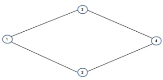
We are looking for the equilibrium points of the first equation of (26)
consid-ering the simple case of a network with four nodes as the one depicted in Fig. 7
[image:28.595.156.324.529.611.2]The evolution of the vector ρis given by ˙
ρ1(t) = − w12+w13ρ1(t) +w21ρ2(t) +w31ρ3(t),
˙
ρ2(t) = w12ρ1(t)− w21+w24ρ2(t) +w42ρ4(t),
˙
ρ3(t) = w13ρ1(t)− w31+w34ρ3(t) +w43ρ4(t),
˙
ρ4(t) = w24ρ2(t) +w34ρ3(t)− w42+w43ρ4(t).
(27)
Case 1
Assume thatw12>0, w31>0, w24>0, w43>0. If
|ε|>maxρ4 w43 w12−
w43 w24
, ρ4 w43 w24−
1, ρ4 w43 w31 −
w43 w12
, ρ4 1− w43 w31
,
then the system to solve is
˙
ρ1(t) = −w12ρ1(t) +w31ρ3(t),
˙
ρ2(t) = w12ρ1(t)−w24ρ2(t),
˙
ρ3(t) = −w31ρ3(t) +w43ρ4(t),
˙
ρ4(t) = w24ρ2(t)−w43ρ4(t),
(28)
that is zero in
ρ4 w43 w12
, ρ4 w43 w24
, ρ4 w43 w31
, ρ4, w12, w24, w31, w43
. (29)
In the following we consider only the values ofw12, w24, w31, w43because their
symmetricw21, w42, w13, w34 are always zero according to Remark 6.1.
Assume thatw12>0, w31>0, w24>0, w43= 0. If|ε|>1, then the system is
zero in
0,0,0,1, w12, w31w24,0. (30)
Case 3
For w12 >0, w31 > 0, w24 = 0, w43 = 0. If |ε| > max{ρ4,1−ρ4}, then the
system is zero in
0,1−ρ4,0, ρ4, w12, w31,0,0
. (31)
Case 4
Forw12>0, w31 = 0, w24= 0, w43= 0. if |ε|>max{ρ4, ρ3,1−ρ4−ρ3} then
the system is zero in
0,1−ρ4−ρ3, ρ3, ρ4, w12. (32)
Case 5
Assume that allwij = 0∀j ∈N(i). If
|ε|>max{ρ1−ρ2, ρ2−ρ4, ρ3−ρ1, ρ4−ρ3},
then the equilibrium point of the system is
(1−ρ2−ρ3−ρ4, ρ2, ρ3, ρ4,w) = (ρ1, ρ2, ρ3, ρ4,0), (33)
Remark 6.2 Note that the equilibria in cases 2,3,4,5 can be obtained as
limits of the equilibrium in case 1. Indeed if we let w43 →0 we end up with
equilibrium (30)and since P4i=1ρi = 1,ρ4= 1. Ifw43→0 andw24 →0 we
obtain equilibrium (31) where we denoted by 1−ρ4 the indeterminate form
ρ4ww4324, taking into account the conservation of mass. Furthermore ifw31→0,
w24→0andw43→0we get equilibrium (32), where we call the indeterminate
formsρ4ww4331 andρ4
w43
w24 respectivelyρ3 and1−ρ4−ρ3 for the same reason as before.
Finally letting all wij → 0 we end up with equilibrium (33), in which ρ2,
ρ3, and 1−ρ2−ρ3−ρ4 denote the indeterminate forms ρ4ww4324, ρ4
w43
w31, and
ρ4ww4312 that respect the conservation of mass.
Moreover, our choice of taking w12 > 0, w31 > 0, w24 >0, w43 >0 and not
other wij is completely arbitrary, indeed taking any 4 non symmetricwij >0
we will end up with an equilibrium of the same type of (29).
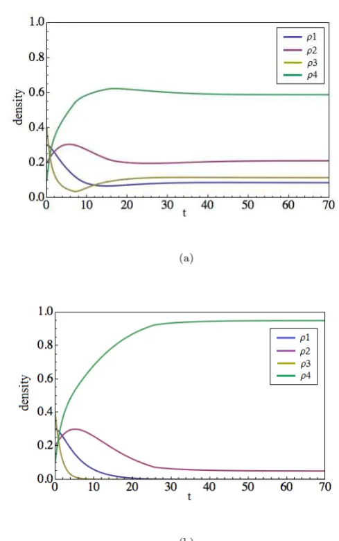
In the following numerical simulations we show the behavior of the system for
(a)
(b)
Fig. 8 Numerical simulations of the system converging to the equilibria in case 1 (Fig. 8(a))
and case 3 (Fig. 8(b))
[image:32.595.104.349.95.485.2]to equilibrium (31).
6.3 Stability
In the following subsection we show that also in the presence of the play
op-erator we converge to the equilibrium fort → ∞. Before doing this we make a further assumption for the manifold as defined next.
The global equilibrium manifoldM in this case is the union of different equi-librium manifolds
M =
5
[
z=1
Mz, (34)
where ¯Mzdenotes the manifold whose points are equilibria relative to thez-th case.
Assumption 2
Let M be given as in (34), s > 0 and S = {ρ : dist(ρ, M) < s}. For all
ρ= (ρ, w)∈S\M, there existsξ∈ΠMρsuch that the valueval[λ]is negative for everyλ= (ρ−ξ), namely
val[λ] = inf
u{λ·(I−∂ρξ(ρ(t))) ˙ρ(t)
T}<0. (35)
This assumption is analogous to the attainability (21) in the presence of
Theorem 6.1 Let Assumption 2 hold true. Thenρ(t)converges
asymptomat-ically toM, namely
lim
t→+∞dist(ρ, M) = 0. (36)
Proof.:Letρa solution of (26) with initial valueρ(0)∈S\M. Set
τ={inft >0 :ρ(t)∈M} ≤ ∞and letV(ρ(t)) =dist(ρ, M). We compute: ˙
V(ρ(t)) =d
dt
kρ(t)−ξ(ρ(t))k
=
1
kρ(t)−ξ(ρ(t))k
ρ(t)−ξ(ρ(t)) I−∂ρξ(ρ(t))
˙
ρ(t)T
<0
by (35). Then the solution ρof (26) is asymptotically stable and we have a
global equilibrium. ⊓⊔
In the following we deal with some examples of convergence to the equilibria
in differentMzusing the decentralized control u∗ij = (ρi−ρj)+.
At first we suppose that ε > 1 thus for all t, w(t) satisfies the conditions in case 2. The system to study is
˙
ρ1(t) =−w12(t)ρ1(t) +w31(t)ρ3(t),
˙
ρ2(t) =w12(t)ρ1(t) +w24(t)ρ2(t),
˙
ρ3(t) =−w31(t)ρ3(t),
˙
ρ4(t) =w24(t)ρ2(t).
(37)
From the assumption on thewij we have
∃c >0 :wij(t)> c∀t≥0.
Then considering the third equation of (37) we have that
ρ1(t)→ρ¯1 with ¯ρ1>0. Thus,
lim
t→+∞ρ˙1(t) = limt→+∞−w12(t)¯ρ1+ limt→+∞w31(t)ρ3(t)6= 0. (38)
This is a contradiction as the left hand side should be equal to zero. Hence
limt→+∞ρ1(t) = 0. With similar argument also limt→+∞ρ2(t) = 0. For the
mass conservation ρ4(t) → 1 for t → +∞ hence we obtain the equilibrium
point (30).
Assuming now thatε >max{ρ4(0),1−ρ4(0)}andw(0) satisfies the conditions
in case 3, the system becomes
˙
ρ1(t) =−w12(t)ρ1(t) +w31(t)ρ3(t),
˙
ρ2(t) =w12(t)ρ1(t),
˙
ρ3(t) =−w31(t)ρ3(t),
˙
ρ4(t) = 0,
(39)
for allt∈[0,¯t[ where
¯
t= sup{t≥0 :u∗12+ε > w12(t)≡w12(0)>0, u∗31+ε >w31(t)≡w31(0)>0, w24≡0, w43≡0}.
We will now prove that ¯t= +∞.
Let us suppose by contradiction that ¯t <+∞. Obviouslyρ4(t)≡ρ4(0) in [0,t¯[.
Using the hypothesis overwij we have thatρ3(t) =e−w31(0)tρ3(0) in [0,¯t[ and
thusρ3decreases. Moreoverρ2is increasing.
andρ3ցthenρ4−ρ3ր. This difference is always less than or equal toρ4and
thus it is less thanε. By the continuity of ρ, lim
t→¯t(ρ4(t)−ρ3(t))< ε. Therefore
w43does not change and remains equal to 0 in [0,¯t].
Let us now considerρ2−ρ4. By (39), in [0,¯t[ρ2ր, thusρ2−ρ4increases and
is less than 1−ρ4< ε. By the previous continuity argumentw24≡0 in [0,t¯].
From the last two results we can conclude thatρ4(t)≡ρ4(0) in [0,¯t].
Considering ρ3−ρ1 we have that, ifρ3−ρ1 ցin [0,¯t[, the last difference is
greater than−ρ1=ρ4−1+ρ3+ρ2> ρ4−1>−ε. This impliesε > ρ1and thus
using the continuity argumentw31(t) =w31(0)>0 in [0,¯t]. Instead ifρ3−ρ1ր
it is always less thatρ3<1−ρ4 < ε. Then as beforew31(t) =w31(0)>0 in
[0,¯t]. From the last one andw43≡0 we concludeρ3(t) =ρ3(0)e−w31(0)tin [0,t¯].
Again if ρ1−ρ2 ց it is greater than −ρ2 > ρ4 −1 > −ε. Proceeding as
before we conclude that w12(t) = w12(0) > 0 in [0,¯t]. Instead if ρ1−ρ2 ր
reasoning as before we reach the same conclusion, i.e,w12(t) =w12(0)>0 in
[0,¯t].
Hence we have proven that in ¯t, the same conditions valid in the interval [0,t¯[, hold. Therefore there existsδ >0 such that in [0,t¯+δ],wij(t) are the same as int= 0. This is a contradiction as ¯tis a supremum, thus we conclude ¯t= +∞.
We will now prove that the system converges to equilibrium (31). From the
contradiction, we suppose thatρ1(t)→ρ¯1 with ¯ρ1>0. Thus,
lim
t→+∞ρ˙1(t) = limt→+∞−w12(t)¯ρ16= 0. (40)
This is a contradiction as it should be equal to zero. Hence limt→+∞ρ1(t) = 0.
Regardingρ4and ρ2, the first is constant and limt→+∞ρ2(t) = ¯ρ2>0. From
the mass conservation ¯ρ2= 1−ρ¯4hence we obtain an equilibrium point as in
(31).
Using similar arguments, ifεis like in case 4 and 5 we will converge to equi-libria (32) and (33) respectively.
The above procedure can be extended to the case whereεis such that for all
twe have four non symmetric wij>0 like in case 1.
Note also that the decentralized control u∗
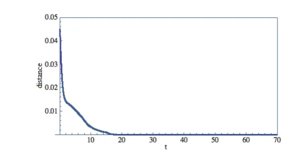
ij = (ρi −ρj)+ satisfies Assump-tion 2, indeed the funcAssump-tionV(ρ(t)) is strictly decreasing along the trajectories (see Fig. 9).
As a consequence, the distance ofρfrom the manifoldM is a Lyapunov func-tion and thus Theorem 6.1 holds true.
The picture below (Fig. 9) displays the distance ofρ from the manifoldM1
as function of time. It is visually clear that the time plot is decreasing in
Fig. 9 The distance ofρfrom the manifoldM1.
7 Conclusions
In this paper we study a decentralized routing problem defined over a network.
We show that by reformulating the problem as a mean-field game, we obtain a
consensus dynamics on the densities. Using a state space extension approach
we recast the problem in the framework of optimal control. We give an explicit
expression of a suitable current cost function in order to obtain a preassigned
optimal decentralized control. We provide conditions for the convergence to
both to local and global consensus. In the presence of a play operator, we prove
that the same control does not guarantee convergence to a consensus point.
In this case, we characterize the set of equilibrium points for the hysteretic
system and prove its asymptotic stability.
Acknowledgements The work has been developed within the OptHySYS project of the
[image:38.595.82.376.81.238.2]period of R. Maggistro at the Department of Automatic Control and Systems Engineering,
References
1. Garavello M., Piccoli, B.: Traffic Flow on Networks. Amer. Inst. Math. Sci. Springfield
(2006)
2. Engel, K-J., Kramar, F.M., Nagel, R., Sikolya, E.: Vertex control of flows in networks.
Netw. Heterog. Media 3(4), 709-722 (2008)
3. Ren, W., Beard, R. W.: Distributed consensus in multi-vehicle cooperative control.
Springer, London (2008)
4. Bauso, D., Zhang, X., Papachristodoulou, A.: Density Flow over Networks via
Mean-Field Game. IEEE Trans. Automat. Control, DOI:10.1109/TAC.2016.2584979, (2016)
5. Bauso, D., Blanchini, F., Giarr´e, L., Pesenti, R.: The linear saturated decentralized
strategy for constrained flow control is asymptotically optimal. Automatica 49(7),
2206-2212 (2013)
6. Como, G., Savla, K., Acemoglu, D., Dahleh, M., Frazzoli, E.: Distributed robust routing
in dynamical networks-Part I: Locally responsive policies and weak resilience. IEEE
Trans. Automat. Control 58(2), 317-332 (2013)
7. Como, G., Savla, K., Acemoglu, D., Dahleh, M., Frazzoli, E.: Distributed robust routing
in dynamical networks-Part II: strong resilience, equilibrium selection and cascaded
failures. IEEE Trans. Automat. Control 58(2), 333-348 (2013)
8. Kelly, F. P., Maulloo, A. K., Tan, D. K. H.: Rate control for communication networks:
Shadow prices, proportional fairness and stability. J. Oper. Res. Soc. 49, 237-252 (1998)
9. Basna, R., Hilbert, A., Kolokoltsov, V.: An Epsilon Nash Equilibrium For Non-Linear
Markov Games of Mean-Field-Type on Finite Spaces. Commun. Stoch. Anal. 8(4),
449-468 (2014)
10. Bagagiolo, F., Bauso, D.: Objective function design for robust optimality of linear
con-trol under state-constraints and uncertainty. ESAIM Concon-trol Optim. Calc. Var. 17(1),
155-177 (2011)
11. Carmona, R., Delarue, F., Lachapelle, A.: Control of McKean-Vlasov dynamics versus
12. Ceragioli, F., De Persis, C., Frasca, P.: Discontinuities and hysteresis in quantized
av-erage consensus. Automatica 47(9), 1916-1928 (2011)
13. Huang, M.Y., Caines, P.E., Malham´e, R.P.: Individual and Mass Behaviour in Large
Population Stochastic Wireless Power Control Problems: Centralized and Nash
Equi-librium Solutions. IEEE Conference on Decision and Control, HI, USA, 98-103 (2003)
14. Huang, M.Y., Caines, P.E., Malham´e, R.P.: Large population cost-coupled LQG
prob-lems with non-uniform agents: individual-mass behaviour and decentralizedε-Nash
equi-libria. IEEE Trans. Automat. Control 52(9), 1560-1571 (2007)
15. Lasry, J.-M., Lions, P.-L.: Jeux `a champ moyen. I Le cas stationnaire. C. R. Math.
Acad. Sci. Paris 343(9), 619-625 (2006)
16. Lasry, J.-M., Lions, P.-L.: Mean field games. Jpn. J. Math. 2 , 229-260 (2007)
17. Weintraub, G. Y., Benkard, C., Van Roy, B.: Oblivious Equilibrium: A Mean Field
Approximation for Large-Scale Dynamic Games. Advances in Neural Information
Pro-cessing Systems, MIT Press (2005)
18. Achdou, Y., Camilli, F., Capuzzo Dolcetta, I.: Mean field games: numerical methods for
the planning problem. SIAM J. Control Optim. 50(1), 77-109 (2012)
19. Gueant, O., Lasry, J.-M., Lions, P.-L.: Mean field games and applications, Springer,
Paris-Princeton Lectures, 1-66 (2010)
20. Lachapelle, A., Salomon, J., Turinici, G.: Computation of mean-field equilibria in
eco-nomics.Math. Models Methods Appl. Sci. 20(4), 1-22 (2010)
21. Bauso, D., Zhu, Q., Basar, T.: Mixed integer optimal compensation: decompositions and
mean-field approximations. Proceeding of 2012 American control conference, Montreal,
Canada (2012)
22. Bagagiolo, F., Bauso, D.: Mean-field games and dynamic demand management in power
grids. Dyn. Games Appl. 4(2), 155-176 (2014)
23. Achdou, Y., Capuzzo Dolcetta, I.: Mean field games: numerical methods. SIAM J.
Nu-mer. Anal. 48(3), 1136-1162 (2010)
24. Casti, J.: On the general Inverse Problem Of Optimal Control Theory. J. Optim. Theory
25. Chitour, Y., Jean, F., Mason, P.: Optimal Control Models of Goal-Oriented Human
Locomotion. SIAM J. Control Optim. 50(1), 147-170 (2012)
26. Krasnoselskii, M. A., Pokrovskii, A. V.: Systems with hysteresis, Springer, Berlin (1989)
27. Visintin, A.: Differential Models of Hysteresis, Springer-Verlag, Berlin (1994)
28. Wardrop, J. G.: Some theoretical aspects of road traffic research. Proc. Inst. Civil Engi.