arXiv:1801.00433v1 [astro-ph.SR] 1 Jan 2018
M. B. Kors´os , , S. Poedts , N. Gyenge , , M. K. Georgoulis , S. Yu , S. K. Bisoi , Y. Yan , M. S.
Ruderman1
& R. Erd´elyi1
[email protected], [email protected],
ABSTRACT
We apply a novel pre-flare tracking of sunspot groups towards improving the estima-tion of flare onset time by focusing on the evoluestima-tion of the 3D magnetic field construc-tion of AR 11429. The 3D magnetic structure is based on potential field extrapolaconstruc-tion encompassing a vertical range from the photosphere through the chromosphere and transition region into the low corona. The basis of our proxy measure of activity
pre-diction is the so-called weighted horizontal gradient of magnetic field (W GM) defined
between spots of opposite polarities close to the polarity inversion line of an active region. The temporal variation of the distance of the barycenter of the opposite po-larities is also found to possess potentially important diagnostic information about the flare onset time estimation as function of height similar to its counterpart introduced initially in an application at the photosphere only in Korsos et al. (2015). We apply the photospheric pre-flare behavioural patterns of sunspot groups to the evolution of their associated 3D-constructed AR 11429 as function of height. We found that at a certain height in the lower solar atmosphere the onset time may be estimated much earlier than at the photosphere or at any other heights. Therefore, we present a tool and recipe that may potentially identify the optimum height for flare prognostic in the solar atmosphere allowing to improve our flare prediction capability and capacity.
Subject headings: Sun: Solar flare - Magnetic field extrapolation
1Solar Physics & Space Plasma Research Center (SP2RC), School of Mathematics and Statistics, University of Sheffield, Hounsfield Road, S3 7RH, UK
2New Jersey Institute of Technology, Center for Solar-Terrestrial Research, 323 Martin Luther King Blvd Newark, NJ 07102, United States
3Key Laboratory of Solar Activity, National Astronomical Observatories, Chinese Academy of Sciences, Beijing,
China
4Center for Mathematical Plasma Astrophysics, KU Leuven, Celestijnenlaan 200B, 3001 Leuven, Belgium
5Research Center for Astronomy and Applied Mathematics of the Academy of Athens, 4 Soranou Efesiou Street,
11527 Athens
6DHO, Konkoly Astronomical Institute, Research Centre for Astronomy and Earth Sciences, Hungarian Academy
1. Introduction
The 3D magnetic field structure of an AR is a key to obtain a more accurate information about the pre-flare evolution of a flaring AR. However, to construct an accurate 3D magnetic skeleton of an AR is a challenging task, see e.g. Wiegelmann & Sakurai (2012). To accomplish this, one may need to measure the magnetic field at a number of heights. However, even nowadays, there are no routinely carried out direct measurements of the solar magnetic field in the solar atmosphere except only at the photosphere, see e.g. the magnetic field observations by SDO/HMI. Measuring routinely the magnetic field higher up in the solar atmosphere proved to be far too challenging
because of a number of technical reasons, see e.g. Solanki et al. (2003) and the follow-up debate
by Judge (2009). Therefore, we may need to develop other complementary theoretical tools, that capture the key features of the 3D magnetic structure of an AR in the (lower) solar atmosphere. A frequently used such tool is magnetic field extrapolation based on photospheric measurements, see e.g. Wiegelmann & Sakurai (2012). The method employs the approximation that the solar corona
is considered to be in low-β plasma state, or in other words, the magnetic pressure dominates over
the pressure in the plasma. From this, we may approximate the plasma being in force-free (FF) state satisfying
j×B= 0. (1)
Here,j= µ01 ▽×B is the electric current density, Bthe magnetic field andµ0 is the magnetic
permeability of free space. This approximation may be a good one for describing the state of the coronal magnetic field. However, many studies claim (for good reasons) that the FF approximation is not reliable below the transition region, especially in the photosphere. Equation (1) can be
satisfied by j = ▽×B = 0, where the current density vanishes everywhere. This is called a
potential field (PF). Another option is when j || B, that can be rewritten as ▽×B = α ~B and
B·▽α = 0, where α is the FF parameter. When α is constant along B everywhere in a given
volume, it is the linear FF field (LFFF) approximation, otherwise αmay be a spatially dependent
scalar function, in which case we have the nonlinear FF field (NLFFF) approximation.
2. Analysis
Kors´os et al. (2015), hereafter K15, introduced a new parameter that may more accurately
characterise the pre-flare evolution of the photospheric magnetic field of ARs. This is the weighted
horizontal gradient of the magnetic field (W GM) between nearby groups of spots of opposite
mag-netic polarities closest to the polarity inversion line. With an empirical analyses, for all the observed flare cases between 1996-2010 that satisfy certain selection criteria (for that see K15), they discov-ered two typical pre-flare patterns for higher than M5 GOES flare-classes: (i) The pre-flare behavior
of the W GM itself exhibits characteristic and unique patterns: steep rise, high maximum and a
gradual decrease prior to flaring. (ii) There is a U-shaped typical pre-flare pattern during the com-pressing and diverging motion in the distance value of the area-weighted barycenters of opposite polarities preceding the flare onset. Also, K15 found, surprisingly, that if any one of these two typical pre-flare behaviours is missing then no flare occurs.
Based on the empirical study of K15, a further tool was developed for estimating the flare onset time: if one can identify the time when the distance between the two barycentres of the area-weighted opposite polarities begins to grow again after the compression phase of the evolution, then one may be able to estimate the onset time of the flare by Eq. (3) of K15. With the
aim to improve the efficiency of the onset time estimation capability of the W GM method that
is based on the observed photospheric dynamics of pre-flare, we now propose to investigate the
two pre-flare signatures not only at the photosphere but higher up in the lower solar atmosphere,
i.e. in the Interface Region and low corona in a 3D-constructed magnetic structure for an AR.
Implementing SDO/HMI line of sight magnetogram (and imaging) observations in the construction of the magnetic mapping of ARs may be a fruitful task. This procedure may also be cumbersome
and computationally very expensive. Based on the W GM method, we test now the feasibility of
estimating the flare onset time on the magnetic mapping of AR 11429 using one of the simplest 3D magnetic constructions, namelly the PF exploration (see Fig. 2a). This way, if it works and applied routinely, a new data catalogue may be established, for further analysis. This catalogue which is based on the 3D magnetic data would contain valuable information on position, area and magnetic field/flux for each sunspot across the lower solar atmosphere.
In order to test the concept, here, let us now apply theW GM method and track the temporal
variation ofW GM, distance of the area-weighted barycentre of the opposite polarities and the net
flux at various heights for pre-flare dynamic studies for AR 11429 which produced one X5.4 (on 2012-03-07 00:24) and two M-class flares (M6.3 and M8.4 flares on 2012-03-09 03:53 and 2012-03-10 17:44). The investigation of the pre-flare dynamics is applied to the 3D construction of the AR
between 6-12 March. Note, we cannot investigate the X5.4 flare because the limits of the W GM
method (e.g. the X5.4 flare occurred close to the East limb).
In the first step, as one ascends with a step-size of 100 km higher in the solar atmosphere and
reaches the level of 2 Mm above the photosphere, following the application of the W GM method
the W GM (the increasing, maximum and after the decreasing phase of W GM), and, the distance
(evolving during the full converging-diverging motion of area-weighted barycenters) prior to flare(s).
Furthermore, we also find that the evolution ofW GM and distance changes remarkably as function
of height (see Fig. 1a-c).
In short, as we reach ∼0.4-0.6 Mm heights in the solar atmosphere, we see the beginning of
the converging-diverging motion of the distance startsearlier than at the photospheric level.
3. Result
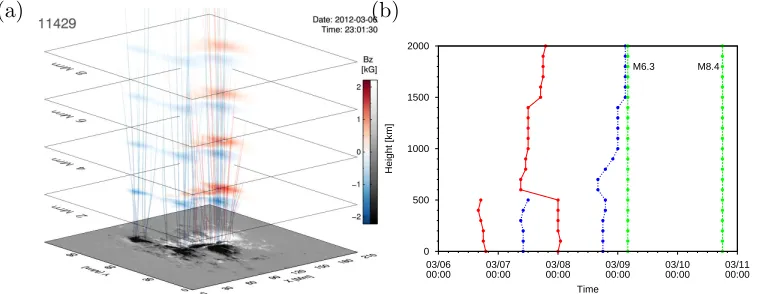
While applying the W GM method to the PF extrapolated structure of AR 11429 we notice
that the starting time of the approaching phase changes as function of height, as visualized in
Fig. 2. Here, we plot the start of the converging phase (red lines) and the moment of time of the minimum distance of barycentres (blue lines) as function of height. We notice that in the case of the M6.3 flare at about 0.4 Mm level, and, in the case of M8.4 flare at about 0.6 Mm, the converging phase starts much earlier and reaches the minimum point also earlier than it does at the photosphere or at other heights. From this behaviour we may conclude that the flare onset times (by using the empirical Eq. 3 from K15 or otherwise) could be estimated sooner at certain heights than at photosphere or in the corona. In summary, identifying this optimum height in the solar atmosphere for a given AR may increase the time window elapsing prior to a flare. If this conclusion is confirmed by using a larger, statistically significant sample of ARs containing flare eruptions this would be a significant progress.
Acknowledgement: MBK, NGY, MSR and RE are grateful to the U. of Sheffield, STFC and the Royal Society (UK) for the support.
YY is supported by NSFC grant.
REFERENCES
Judge, P. G. 2009, A&A, 493, 1121J
Kors´os, M. B., Ludm´any, A., Erd´elyi, R., Baranyi, T., 2015, ApJ, 802, L21
Solanki, S. K., Lagg, A., Woch, J., Krupp, N., & Collados, M. 2003, Nature, 425, 692-695
Wiegelmann, T. & Sakurai, T. 2012, Living Reviews in Solar Physics, 9, 5, 49 pp
4.0⋅105 8.0⋅105 1.2⋅106 1.6⋅106 2.0⋅106
03/06 03/08 03/10 03/12
WG
M
[Wb/m]
X5.4 M6.3 M8.4
1.0⋅107 2.0⋅107 3.0⋅107
03/06 03/08 03/10 03/12
Distant [m]
1.0⋅1013 2.0⋅1013 3.0⋅1013
03/06 03/08 03/10 03/12
Flux [Wb] Time (a) 4.0⋅105 8.0⋅105 1.2⋅106 1.6⋅106 2.0⋅106
03/07 03/09 03/11
WG
M
[Wb/m]
X5.4 M6.3 M8.4
1.6⋅107 2.0⋅107 2.4⋅107 2.8⋅107 3.2⋅107
03/07 03/09 03/11
Distant [m]
1.0⋅1013 2.0⋅1013 3.0⋅1013 4.0⋅1013
03/07 03/09 03/11
Flux [Wb] Time (b) 3.0⋅105 6.0⋅105 9.0⋅105 1.2⋅106
03/07 03/09 03/11
WG
M
[Wb/m]
X5.4 M6.3 M8.4
1.6⋅107 2.0⋅107 2.4⋅107 2.8⋅107
03/07 03/09 03/11
Distant [m]
1.0⋅1013 2.0⋅1013 3.0⋅1013
03/07 03/09 03/11
Flux [Wb]
Time
[image:5.612.114.500.125.319.2](c)
Fig. 1.— : Top panels are the variation of W GM, middle panels depict the evolution of distance
between the area-weighted barycenters of the spots of opposite polarities and the bottom panels show the unsigned flux of all spots at various heights as function of time. Column (a) is at photospheric level; (b) at 0.5 Mm and (c) at 1Mm levels, respectively, in the solar atmosphere. The red parabolae highlight the typical converging-diverging motion (U-shape) between the two area-weighted centres of the opposite polarities prior to flare(s). The blue/green vertical lines represent the X/two M-class flares onset times.
(a) 0 500 1000 1500 2000 03/06
00:00 03/0700:00 03/0800:00 03/0900:00 03/1000:00 03/1100:00
Height [km]
Time
M6.3 M8.4
(b)
[image:5.612.112.493.468.615.2]