This is a repository copy of Reconstruction of a source domain from boundary measurements.
White Rose Research Online URL for this paper: http://eprints.whiterose.ac.uk/110343/
Version: Accepted Version
Article:
Bin-Mohsin, B and Lesnic, D (2017) Reconstruction of a source domain from boundary measurements. Applied Mathematical Modelling, 45. pp. 925-939. ISSN 0307-904X https://doi.org/10.1016/j.apm.2017.01.021
Crown Copyright © 2017 Published by Elsevier Inc. Licensed under the Creative Commons Attribution-NonCommercial-NoDerivatives 4.0 International
http://creativecommons.org/licenses/by-nc-nd/4.0/
eprints@whiterose.ac.uk https://eprints.whiterose.ac.uk/ Reuse
Unless indicated otherwise, fulltext items are protected by copyright with all rights reserved. The copyright exception in section 29 of the Copyright, Designs and Patents Act 1988 allows the making of a single copy solely for the purpose of non-commercial research or private study within the limits of fair dealing. The publisher or other rights-holder may allow further reproduction and re-use of this version - refer to the White Rose Research Online record for this item. Where records identify the publisher as the copyright holder, users can verify any specific terms of use on the publisher’s website.
Takedown
If you consider content in White Rose Research Online to be in breach of UK law, please notify us by
Reconstruction of a source domain from
boundary measurements
B. Bin-Mohsin
1and D. Lesnic
21
Department of Mathematics, College of Science, King Saud University,
PO. Box 2455 Riyadh 11451, Saudi Arabia
2
Department of Applied Mathematics, University of Leeds, Leeds LS2 9JT,
UK
balmohsen@ksu.edu.sa, amt5ld@maths.leeds.ac.uk
Abstract
Inverse and ill-posed problems which consist of reconstructing the unknown support of a source from a single pair of exterior boundary Cauchy data are investigated. The underlying dependent variable, e.g. potential, temperature or pressure, may satisfy the Laplace, Poisson, Helmholtz or modified Helmholtz partial differential equations (PDEs). For constant coefficients, the solutions of these elliptic PDEs are sought as linear combinations of explicitly available fundamental solutions (free-space Greens functions), as in the method of fundamental solutions (MFS). Prior to this application of the MFS, the free-term inhomogeneity represented by the intensity of the source is removed by the method of particular solutions. The resulting transmission problem then recasts as that of determining the interface between composite materials. In order to ensure a unique solution, the unknown source domain is assumed to be star-shaped. This in turn enables its boundary to be parametrised by the radial coordinate, as a function of the polar or, spherical angles. The problem is nonlinear and the numerical solution which minimizes the gap between the measured and the computed data is achieved using the Matlab toolbox routine lsqnonlin which is designed to
minimize a sum of squares starting from an initial guess and with no gradient required to be supplied by the user. Simple bounds on the variables can also be prescribed. Since the inverse problem is still ill-posed with respect to small errors in the data and possibly additional ill-conditioning introduced by the spectral feature of the MFS approximation, the least-squares functional which is minimized needs to be augmented with regularizing penalty terms on the MFS coefficients and on the radial function for a stable estimation of these couple of unknowns. Thorough numerical investigations are undertaken for retrieving regular and irregular shapes of the source support from both exact and noisy input data.
1
Introduction
The determination of the support of a source contained in a given underlying medium from knowledge of the Cauchy data on the exterior boundary is investigated. As a practical proce-dure it resembles non-destructive testing of materials. Closely related to this inverse problem is that of detecting an unknown anomaly (defect) contained in a given domain from tomo-graphic scaning on the skin/surface of the specimen under investigation. The inverse source problem investigated in this study is also closely related to the inverse potential gravimetry problem in which one is interested in determining the density inside the Earth from gravi-metric measurements on its surface, see Novikov (1938) and Isakov (1990). Another possible application of our inverse source domain identification could be electroencephalography, see Jourhmane (1993), which is a non-invasive scanning tomographic technique of imaging/ mea-suring the electrical activity of the brain.
Prior to the present study, there were a few works which investigated the reconstruc-tion of a source domain from boundary measurements from, mainly theoretical perspec-tives. The underlying medium was subject to various excitations such as electrical, i.e. Laplace’s/Poisson’s equation for the potential in electroencephalography, see Ito and Liu (2013) and Canelas et al. (2014), thermal, i.e. the modified Helmholtz equation for the temperature in a fin, see Mamud et al. (2014), or acoustics, i.e. the Helmholtz equation for the pressure, see Ikehata (1999).
In this paper, the aim is to reconstruct numerically in a stable and accurate manner the source domain entering all the aforementioned stationary elliptic fields. We employ a com-bined meshless technique with nonlinear optimization which recently has proved successful in a related study by the authors, see Bin-Mohsin and Lesnic (2014), concerned with the reconstruction of an inhomogeneity entering the modified Helmholtz equation.
We mention that for the potential field our problem and methodology is similar to that developed recently by Martins (2012). However, in our study we investigate Helmhholtz-type equations as well. We also do not avoid ill-conditioning by parameterising the unknown shape with a finite set of trigonometric polynomials, but rather keep the shape general and deal with it using regularization.
The plan of the paper is as follows. In Section 2, we introduce the mathematical formu-lation of the inverse source domain problem and state the available uniqueness results. In Section 3, we describe the MFS with the inhomogeneity removal, as well as the nonlinear minimization proposed for reconstructing the star-shape support of the unknown source. Section 4 presents and discusses thorough numerical results in which the convergence of the objective function with the number of iterations is analysed. Also, the stability of the nu-merical solution with respect to noise in the input data is investigated. Finally, Section 5 presents the conclusions of the work.
2
Mathematical formulation
We consider the inverse problem of determining an unknown source domain inhomogeneity Ω2 compactly contained in a bounded domain Ω ⊂ Rd, d = 2,3, appearing in the elliptic
equation
where χΩ2 denotes the characteristic function of the domain Ω2, u∈H
1(Ω) is the potential,
F1, F2 ∈ L2(Ω) are given source intensities which are assumed to be known and k is a
known real or complex number or function. We assume that all the domains involved have a Lipschitz regularity boundary. From equation (1) one can observe that Ω2 represents the
support of the source function F2 if F1 ≡0.
By defining
u=:
u1 in Ω1 := Ω\Ω2,
u2 in Ω2, (2)
equation (1) can be rewritten as the following transmission problem:
∇2u
1 +k2u1 =F1 in Ω1, (3)
∇2u2 +k2u2 =F2 in Ω2, (4)
u1 =u2 on∂Ω2, (5)
∂u1
∂n = ∂u2
∂n on∂Ω2, (6)
wherendenotes the outward unit normal to the boundary. It might be also useful to remark that the right-hand side of equation (1) can be re-expressed as F1χΩ1 +F2χΩ2.
Associated to (3)-(6) we also have prescribed one pair of Cauchy boundary data on ∂Ω, namely,
u1 =f on∂Ω, (7)
∂u1
∂n =g on∂Ω. (8)
The inverse problem then requires the determination of the triplet solution (u1, u2, ∂Ω2)
sat-isfying equations (3)-(8). Such an important inverse problems arises in gravimetry, where one would like to determine the density of the Earth from the Cauchy data measurements of the gravity and its normal derivative on its surface. Other related obstacle identification problems and results in various fields are discussed by El-Badia and Ha-Duong (2000) and Isakov (2009).
The reconstruction of the source domain Ω2 is nonlinear and ill-posed. One serious issue
here is the uniqueness of solution from a single pair of Cauchy data (7) and (8). Unlike the inverse conductivity problem of electrical impedance tomography (EIT) in which the knowledge of the Dirichlet-to-Neumann map suffices to determine uniquely an isotropic con-ductivity, in the problem under investigation a single pair of Cauchy data contains all the information necessary for reconstruction, see Alves et al. (2009), in the sense that any other Cauchy data pair does not add any further information. Thus, one could take, without loss of generality, homogeneous Dirichlet data f ≡ 0 in (7) and non-identically zero Neumann data 06≡g ∈H−1/2(∂Ω) in (8).
The following theorems give the classes of star-shaped, convex and polygonal obstacles for which uniqueness holds.
Theorem 1. Let k = 0 in (1). If F1 and F2 are given real constants, then the inverse
problem (3)-(8) has at most one solution Ω2 in the class of star-shaped domains with respect
to their centre of gravity, i.e. barycentre.
In the case of the modified Helmholtz equation, i.e. k=ik′ with k′ ∈
R∗+ in (1), we have the
following uniqueness theorem in the class of convex domains, see Isakov (1990) and Mamud
et al. (2014).
Theorem 2. Let k = ik′ with k′ ∈ R∗
+ in (1). If F1 ≡ 0 and F2 > 0, then the inverse
problem (3)-(8) has at most one solutionΩ2 in the class of convex domains provided that, in
addition, u is prescribed in an interior a priori known ball included in Ω2.
In the absence of this latter interior observation so far, one can only determine the centroid and the effective radius of Ω2.
Finally, in the case of the Helmholtz equation, i.e. k ∈R∗+ in (1), ifF1 ≡0, Ω2 is a polygon
and 0 6= F2 ∈ L2(Ω2) is an unknown function which is locally Holder continuous with
ex-ponent α∈(0,1] in the neighbourhood of each vetex of ∂Ω2, then one can recover uniquely
the convex hull [Ω2] of Ω2 in the problem (3)-(8), see Ikehata (1999).
Once the uniqueness of solution has been discussed, the next topic is to reconstruct the source domain Ω2 numerically. Recently, the method of fundamental solutions (MFS) has
proved, see Bin-Mohsin and Lesnic (2012, 2014), and Lesnic and Bin-Mohsin (2012), versatile and easy to use in detecting cavities, rigid inclusions and contact impedance obstacles, as well as inhomogeneities in inverse geometric problems governed by the modified Helmholtz equation. For a recent review of the MFS, as applied to solving inverse geometric problems, see Karageorghis et al. (2011). In this paper, we investigate yet another application of the MFS to reconstruct the source domain Ω2 from the Cauchy data (7) and (8).
3
The method of fundamental solutions (MFS)
Prior to applying the MFS, we need to move the right-hand side source inhomogeneities F1
and F2 in (3) and (4) to the boundary conditions (5)-(8). This is done by finding particular
solutions to (3) and (4), e.g. in the form of the Newton potential for Poisson’s equation when k = 0, see Atkinson (1985). For the general case, we refer to the technique of Alves and Chen (2005), as well as to the references therein. However, as in our investigation the objective is to find the support Ω2 of F2 rather than its value which, in fact, is assumed to
be known, we will consider the particular, but important, case, see Ito and Liu (2013) and Canelas et al. (2014), that F is piecewise constant within Ω, i.e. F1 and F2 are constants
in (3) and (4). Without loss of generality, we can further assume that F1 = 0 and F2 = 1.
Then, equations (3) and (4) become
∇2u1+k2u1 = 0 in Ω1, (9) ∇2u2+k2u2 = 1 in Ω2. (10)
We now decompose
u2 =uh2 +u
p
where the homogeneous part uh
2 satisfies ∇2uh
2 +k2uh2 = 0 in Ω2, (12)
and the inhomogeneous part is just a particular solution of equation (10) (in the whole Rd) given by, see for example Jin and Zheng (2005),
up2(x) = |x|
2
2d , ifk = 0, (13) up2(x) = 1
k2 +
I0(−ik|x|) ifik ∈R∗−
J0(k|x|) ifk ∈R∗+
(x∈R2), (14)
up2(x) = 1
k2 +
( sinh(−ik|x|)
|x| ifik∈R ∗ −
sin(k|x|)
|x| ifk ∈R ∗
+
(x∈R3), (15)
where of course, in the three-dimensional case the limits in (15) are equal to unity at the origin
x= 0. Besides, the functions J0 and I0 denote the Bessel and the modified Bessel functions
of the first kind of order 0, respectively. These special functions are analytical everywhere (including the origin) and in Matlab they are evaluated using routines besselj(0,k*r)(for
J0) and besseli(0,k*r) (for I0).
With the superposition (11), the transmission interface conditions (5) and (6) become
u1 =uh2 +u
p
2 on∂Ω2, (16)
∂u1
∂n = ∂uh
2
∂n + ∂up2
∂n on∂Ω2, (17)
In (17), the normal derivatives of the particular solutions (13)-(15) are given by
∂up2
∂n(x) = x·n
d , ifk = 0, (18) ∂up2
∂n(x) =
(
−ikx·n
|x| I1(−ik|x|) ifik∈R∗−
−kx·n
|x| J1(k|x|) if k∈R ∗
+
(x∈R2), (19)
∂up2 ∂n(x) =
(x·n)
|x|2 h
−ikcosh(−ik|x|)−sinh(|−xik| |x|)i if ik∈R∗−
(x·n)
|x|2 h
kcos(k|x|)− sin(|xk||x|) i
if k∈R∗+
(x∈R3), (20)
forx∈∂Ω2, where J1 andI1 denote the Bessel and the modified Bessel functions of the first
kind of order 1, respectively. They are evaluated using the routines besselj(1,k*r) (for
J1) and besseli(1,k*r) (for I1).
Once the particular solution up2 has been prescribed as in (13)-(15), it can be removed
fromu2 such thatuh2 =u2−up2 satisfies the homogeneous equation (12). Then, we can apply
the MFS for the composite material Ω = Ω1∪Ω2 with Ω1∩Ω2 =∅, as described in Berger
and Karageorghis (1999) for the Laplace equation and in Bin-Mohsin and Lesnic (2011) for Helmholtz-type equations in layered materials. This consists of approximating the solutions
u1 and uh2 of the elliptic homogeneous equations (9) and (12) by finite linear combinations
of fundamental solutions of the form
u1,2N(x) =
2N X
j=1
ajGk(x, ξ1j), x∈Ω1, (21)
uh2,N(x) =
N X
j=1
wherea= (aj)j=1,2N andb= (bj)j=1,N are unknown coefficients to be determined, (ξ j
1)j=1,2N
are source points located outside the annular domain Ω1, (ξ2j)j=1,N are source points located
outside the domain Ω2, and Gk is the fundamental solution of the elliptic equation ∇2u+
k2u= 0 given by, see e.g. Alves and Chen (2005),
Gk(x, ξ) =
ln|x−ξ| ifk = 0
K0(−ik|x−ξ|) ifik ∈R∗−
Y0(k|x−ξ|) ifk ∈R∗+
(x∈R2), (23)
Gk(x, ξ) =
1
|x−ξ| ifk= 0
exp(−ik|x−ξ|)
|x−ξ| ifik ∈R ∗ −
exp(ik|x−ξ|)
|x−ξ| ifk ∈R ∗
+
(x∈R3), (24)
where Y0 and K0 denote the Bessel and the modified Bessel functions of the second kind
of order 0, respectively. These special functions have both a logarithmic singularity at the origin and are evaluated in Matlab using the routines bessely(0,k*r) (for Y0) and besselk(0,k*r) (for K0). One can avoid this singularity at the origin by employing the
non-singular functions J0 and I0 in place of Y0 and K0, respectively, as in the boundary
knot method (BKM) of Chen and Hon (2003). However, the meshless BKM, due to its spectral expansion character, it inherently introduces additional unwanted ill-conditioning and therefore, we do not follow this method here. Instead, we still use a meshless method, namely, the MFS but which by being based on the fundamental solution (23) (or (24)) it exhibits a singularity at the origin (when|x−ξ|= 0). The use of this fundamental solution is further justified rigorously through the denseness results of Bogomolny (1985) and Alves and Chen (2005). Moreover, for simplicity, we do not employ the complex version of the MFS for the Helmholtz equation in two-dimensions based on the Hankel function of the first kind of order zero, namely, H0(1) =J0+iY0 because the singular character is still maintained in the
imaginary part Y0, see Ennenbach and Niemeyer (1996). The only slight difference, which
in practice may happen very rarely, between using Y0 instead of H0(1) is when Y0(k|x−ξ|)
may accidentally become very small giving poor or spurious numerical results, see Barnett and Betcke (2008). We remark that the normalisation constants usually appearing in the fundamental solution (23) (or (24)) have been omitted, as they were incorporated in the unknown coefficients aand bin (21) and (22), respectively. Finally, we mention that all the analysis of the section can easily be extended to include anisotropic homogeneous materials having as their leading part in (1) the anisotropic Laplace-Beltrami operatorPd
i,j=1Kij ∂
2
u ∂xi∂xj,
where (Kij)i,j=1,d denotes the symmetric and positive conductivity tensor. The main change
then is to replace the radial distance |x| by the geodesic distance xTK−1x, see e.g. Jin and
Chen (2006).
In what follows, for simplicity, we explain the inverse methodology in two-dimensions but a similar technique applies to three-dimensional problems as well, see Karageorghis et al. (2013).
The placement of source and collocation points is similar to that employed by Bin-Mohsin and Lesnic (2014), as follows. The source points (ξ1j)j=1,N 6∈Ω are placed on a (fixed) dilated pseudo-boundary∂Ω′ of similar shape as∂Ω. The remaining source points (ξj
1)j=N+1,2N ∈Ω2
and (ξ2j)j=1,N 6∈Ω2 are placed on contraction and dilation (moving) pseudo-boundaries ∂Ω′2
and∂Ω′′
2 similar to∂Ω2 at a distanceδ >0 in the inward and outward directions, respectively.
unit circleB(0; 1). We also assume that the unknown support of the sourceF2is star-shaped
with respect to the origin, i.e.
∂Ω2 ={r(θ)(cos(θ),sin(θ))|θ ∈[0,2π)}, (25)
where r is a 2π-periodic smooth function with values in (0,1). The class of star-shaped domains is required for the uniqueness of a solution in the case k = 0 in Theorem 1, and it is also sufficiently general to model a wide range of shapes, e.g. circles, ellipses, rounded-rectangles, beans, acorns, kites, etc. that are usually tested in the inverse shape detection literature, see e.g. Ivanyshyn and Kress (2006), and Karageorghis and Lesnic (2009). In this setup of particular domains Ω and Ω2, the collocation and source points are uniformly
distributed as follows, see Bin-Mohsin and Lesnic (2014),
Xi = (cos(θi),sin(θi)), Xi+N =ri(cos(θi),sin(θi)), i= 1, N, (26)
ξ1j =R(cos(θj),sin(θj), ξ1j+N = (1−δ)Xj+N, ξ2j = (1 +δ)Xj+N, j = 1, N, (27)
where θi = 2πi/N, ri :=r(θi) fori= 1, N, R >1 and δ∈(0,1).
The unknown radii vector r = (ri)i=1,N, characterising the star-shaped support Ω2,
to-gether with the unknown MFS coefficientsaandb, giving the approximations of the solutions
u1andu2, are simulateneously determined by imposing the transmission conditions (16), (17)
and the Cauchy data (7), (8) at the collocating points (26) in a least-squares sense. This results into minimizing the following (regularized) least-squares nonlinear objective function:
T(a,b,r) :=
u1−f
2
L2(∂Ω)
+ u1
∂n−g
ǫ 2
L2(∂Ω)
+
u1−uh2 −u
p 2 2
L2(∂Ω 2) + ∂u1 ∂n − ∂uh 2 ∂n − ∂up2
∂n 2 L2
(∂Ω2)
+λ1
kak2+kbk2 +λ2kr′k2, (28)
where λ1, λ2 ≥ 0 are regularization parameters to be prescribed. These parameters are
introduced in order to ensure/improve the stability of the nonlinear Tikhonov regularization functional (28). In (28), the Neumann data (8) was input as being a noisy perturbationgǫ of
the exact data g in order to simulate the errors which are inherently present in any practical measurement. The last term in (28) represents a first-order derivative smoothness constraint on our desired shape for Ω2, and is defined as:
kr′k2 =
N X
i=1
ri−ri−1
θi−θi−1
2
, (29)
Introducing the MFS approximations (21) and (22) into (28) results in
T(a,b,r) =
N X
i=1
"2N X
j=1
ajGk(Xi, ξ1j)−f(Xi) #2
+
2N X
i=N+1
"2N X
j=1
aj
∂Gk
∂n (Xi−N, ξ
j
1)−gǫ(Xi−N) #2
+
3N X
i=2N+1
"2N X
j=1
ajGk(Xi−N, ξ1j)−
N X
j=1
bjGk(Xi−N, ξ2j)−u
p
2(Xi−N) #2
+
4N X
i=3N+1
"2N X
j=1
aj
∂Gk
∂n (Xi−2N, ξ
j
1)−
N X
j=1
bj
∂Gk
∂n (Xi−2N, ξ
j
2)−
∂up2
∂n(Xi−2N)
#2
+λ1
(2N X
j=1
a2j +
N X
j=1
b2j
)
+λ2
N X
j=1
(rj−rj−1)2, (30)
where in the last term we have redenoted λ2/(2π/N)2 by λ2.
The above minimization imposes 4N regularised equations in the 4N unknowns (a,b,r). The noisy flux data gǫ is input as
gǫ(Xi) = (1 +ρi p)g(Xi), i= 1, N, (31)
where p represents the percentage of noise and ρi is a pseudo-random noisy variable drawn
from a uniform distribution in [–1, 1] using the MATLAB c command -1+2*rand(1,N). In equation (30), the normal derivative of Gk, via (23) and (24), is given by
∂Gk
∂n (x, ξ) =
(x−ξ)·n
|x−ξ|2 ifk = 0
ik(x−ξ)·n
|x−ξ| K1(−ik|x−ξ|) ifik∈R ∗ −
−k(|xx−−ξξ)|·nY1(k|x−ξ|) if k∈R ∗
+
(x∈R2) (32)
∂Gk
∂n (x, ξ) =
−(|xx−−ξξ)|·3n ifk = 0
(−ik|x−ξ|−1) exp(−ik|x−ξ|)
|x−ξ|3 (x−ξ)·n ifik ∈R∗−
(ik|x−ξ|−1) exp(ik|x−ξ|)
|x−ξ|3 (x−ξ)·n ifk ∈R∗+
(x∈R3) (33)
where Y1 and K1 denote the Bessel and the modified Bessel functions of the second kind
of order 1, respectively. These special functions have are evaluated using the routines
bessely(1,k*r) (for Y1) and besselk(1,k*r) (for K1). In two-dimensions, i.e. d = 2,
the normal n to the boundary ∂Ω1 is given by
n(X) =
(
(cos(θ),sin(θ)), X ∈∂Ω,
1 √
r2(θ)+r′2(θ)(−r
′(θ) sin(θ)−r(θ) cos(θ), r′(θ) cos(θ)−r(θ) sin(θ)), X ∈∂Ω
2. (34)
In this formula, the derivative r′ is approximated using finite differences as
r′(θi)≈
ri−ri−1
θi−θi−1
, i= 1, N. (35)
4
Numerical results and discussion
For simplicity, we consider numerical realisations in the two-dimensions only, with the three-dimensional case being deferred to future work. In all numerical experiments, the initial guess for the unknown vectors aand b are 0, and the initial guess for Ω2 is a circle centred
at the origin of radius 0.7. The Matlab toolbox routine lsqnonlin was run iteratively until a user-specified tolerance of XT OL = 10−6 was achieved, or until when a user-specified
maximum number of iterations MAXCAL= 1000×4N was reached. We have also set the simple bounds on the variable (a,b,r) as the box [−1010,1010]2N ×[−1010,1010]N×(0,1)N.
The choices of the regularization parametersλ1 andλ2 in (30) were based on trial and error,
but nevertheless more research work needs to be undertaken in the future on the rigorous selection of multiple regularization parameters, see e.g. Chen et al. (2008) and Belge et al.
(2002).
In what follows, we take k = 0 for examples 1(a) and 2(a), k′ = 1 for examples 1(b) and
2(b), and k = 1 for examples 1(c) and 2(c). In the subsequent figures 2–6 and 8–11, we graphically represent the initial guess by (− − −), the numerical reconstruction by (− ◦ −) and the exact target by (—–).
4.1
Example 1. (reconstructing a circular source domain)
We consider first retrieving a circle centred at the origin of radiusR0 = 0.5. That is, we seek
the star-shape approximation (25) for the polar radius function
r(θ)≡R0 = 0.5, θ ∈[0,2π). (36)
For the three cases of k that we consider we take the following examples with analytical solutions satisfying equations (9) and (10).
4.1.1 Example 1(a). (k = 0, Laplace’s equation)
In the case k = 0, equations (9), (10) and (12) become
∇2u1 = 0 in Ω1, (37) ∇2u2 = 1 in Ω2, (38) ∇2uh2 = 0 in Ω2. (39)
From (13) we also have that
up2(r, θ) = r
2
4, (r, θ)∈R+×[0,2π). (40) We then take the analytical solutions of the equations (37)-(39) to be given by
u1(r, θ) =
R2 0
2 ln
r R0
+R
2 0
4 , (r, θ)∈(R0,1)×[0,2π), (41)
u2(r, θ) =
r2
4, (r, θ)∈(0, R0)×[0,2π), (42)
Based on (41), the input Cauchy data (7) and (8) are given by
u1(1, θ) =f(θ) =
R2 0
2 ln
1
R0
+ R
2 0
4 , θ ∈[0,2π), (44)
∂u1
∂n(1, θ) = g(θ) = R2
0
2 , θ∈[0,2π), (45) and, based on (25) and (40), the transmission interface conditions (16) and (17) become
u1(r(θ), θ) =uh2(r(θ), θ) +
r2(θ)
4 , θ∈[0,2π), (46)
∂u1
∂n(r(θ), θ) = ∂uh
2
∂n(r(θ), θ) + r(θ)
2 , θ ∈[0,2π). (47) From Theorem 1, we know that (36), (41) and (42) is the unique solution of the problem (37), (38), (44), (45), (5) and (6) in the class of star-shaped domains (25) with respect to the origin. In order to find this solution, we solve numerically, as described in Section 3, the inverse problem given by equations (37), (40), (44)-(47) to retrieve the analytical solution (r(θ), u1(r, θ), uh2(r, θ)) given by equations (36), (41) and (43). Also, once uh2 has
been obtained, equations (11) and (40) yield u2.
4.1.2 Example 1(b). (k=ik′ with k′ ∈R∗
+, modified Helmholtz equation)
In the case k =ik′ with k′ ∈R∗
+, equations (9), (10) and (9) become
∇2u1−k′2u1 = 0 in Ω1, (48) ∇2u2−k′2u2 = 1 in Ω2, (49) ∇2uh
2 −k′2uh2 = 0 in Ω2. (50)
From (13) we also have that
up2(r, θ) = − 1
k′2 +I0(k
′r), (r, θ)
∈R+×[0,2π). (51)
We then take the analytical solutions of the equations (48)-(50) to be given by
u1(r, θ) =B0K0(k′r), (r, θ)∈(R0,1)×[0,2π), (52)
u2(r, θ) =A0I0(k′r)−1, (r, θ)∈(0, R0)×[0,2π), (53)
uh2(r, θ) = (A0−1)I0(k′r)−1 +
1
k′2, (r, θ)∈(0, R0)×[0,2π), (54)
where
A0 =
K1(k′R0)
I0(k′R0)K1(k′R0) +I1(k′R0)K0(k′R0)
,
B0 =−
I1(k′R0)
I0(k′R0)K1(k′R0) +I1(k′R0)K0(k′R0)
, (55)
where we have used that K′
0 =−K1 and I0′ =I1. Based on (52), the input Cauchy data (7)
and (8) are given by
u1(1, θ) = f(θ) =B0K0(k′), θ∈[0,2π), (56)
∂u1
∂n(1, θ) =g(θ) =−B0k
′K
and, based on (25) and (51), the transmission interface conditions (16) and (17) become
u1(r(θ), θ) =uh2(r(θ), θ) +I0(k′r(θ))−
1
k′2, θ ∈[0,2π), (58)
∂u1
∂n(r(θ), θ) = ∂uh
2
∂n(r(θ), θ) +k
′I
1(k′r(θ)), θ ∈[0,2π). (59)
Then, we solve numerically, as described in Section 3, the inverse problem given by equa-tions (48), (50), (56)-(59) to retrieve the analytical solution (r(θ), u1(r, θ), uh2(r, θ)) given by
equations (36), (52) and (54). Also, once uh
2 has been obtained, equations (11) and (51)
yield u2.
4.1.3 Example 1(c). (k ∈R∗+, Helmholtz equation)
In the case k ∈ R∗+, we take the analytical solutions of equations (9), (10) and (12) to be
given by
u1(r, θ) = D0Y0(kr), (r, θ)∈(R0,1)×[0,2π), (60)
u2(r, θ) = C0J0(kr) + 1, (r, θ)∈(0, R0)×[0,2π), (61)
uh2(r, θ) = (C0−1)J0(k′r) + 1−
1
k2, (r, θ)∈(0, R0)×[0,2π), (62)
where
C0 =
Y1(kR0)
Y0(kR0)J1(kR0)−Y1(kR0)J0(kR0)
,
D0 =
J1(kR0)
Y0(kR0)J1(k′R0)−Y1(k′R0)J0(k′R0)
, (63)
where we have used that Y′
0 =−Y1 and J0′ =−J1. From (13) we also have that
up2(r, θ) = 1
k2 +J0(kr), (r, θ)∈R+×[0,2π). (64)
Based on (60), the input Cauchy data (7) and (8) are given by
u1(1, θ) =f(θ) = D0Y0(k), θ∈[0,2π), (65)
∂u1
∂n(1, θ) =g(θ) =−D0kY1(k), θ∈[0,2π), (66)
and, based on (25) and (64), the transmission interface conditions (16) and (17) become
u1(r(θ), θ) =uh2(r(θ), θ) +J0(kr(θ)) +
1
k2, θ∈[0,2π), (67)
∂u1
∂n(r(θ), θ) = ∂uh
2
∂n (r(θ), θ)−kJ1(kr(θ)), θ ∈[0,2π). (68)
Then, we solve numerically, as described in Section 3, the inverse problem given by equa-tions (9), (12), (65)-(68) to retrieve the analytical solution (r(θ), u1(r, θ), uh2(r, θ)) given by
equations (36), (60) and (62). Also, once uh
2 has been obtained, equations (11) and (64)
Initially, we have performed several numerical runs with various values of the input MFS parameters and, for illustrative purposes, we have decided to show in figures 1–6 only a typical selected set of results obtained with δ= 0.5, R= 2 and N = 20.
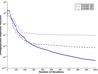
We consider first the case of exact data, i.e. p = 0 in equation (31). Figure 1 shows the unregularised nonlinear least-squares objective function (30) with λ1 = λ2 = 0, as a
function of the number of iterations for examples 1(a)–1(c). From this figure it can be seen that a monotonic decreasing convergence is obtained for all examples. Furthermore, the convergence is faster for example 1(a) than for examples 1(b) and 1(c), but, at present, we have no explanation why this occurs.
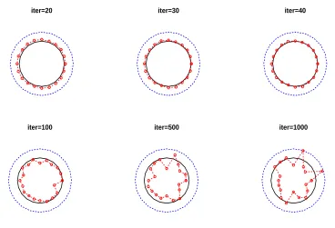
In figure 2, we present the numerically reconstructed inner boundary for various numbers of iterations for no noise and no regularization for example 1(a). From this figure, it can be seen that the reconstructed inner source domain becomes accurate starting from 20 iterations up to 40 iterations. We also observe that as the number of iterations increases over 100, the reconstruction starts to be unstable and inaccurate.
We also add p= 10% noise in the flux g as in equation (31). The numerically obtained results for noisep= 10% with no regularization for various numbers of iterations for example 1(a) are shown in figure 3. From this figure, we note that the numerical solutions become less accurate as the number of iterations increases.
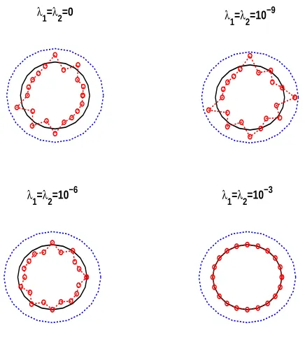
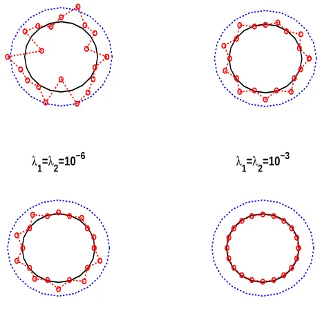
The corresponding regularized results obtained with different values of the regularization parameters λ1 = λ2 ∈ {10−9,10−6,10−3} after 500 iterations are shown in figures 4–6 for
examples 1(a)–1(c), respectively. From these figures, we observe that λ1 =λ2 = 10−3 yields
the most accurate results for all Examples 1(a)–1(c).
Number of iterations
0 100 200 300 400 500 600 700 800 900 1000
Unregularised objective function
10-10 10-8 10-6 10-4 10-2 100 102
[image:13.612.126.469.369.628.2]Example 1(a) Example 1(b) Example 1(c)
iter=20 iter=30 iter=40
[image:14.612.122.482.52.260.2]iter=100 iter=500 iter=1000
Figure 2: The reconstructed inner source domain for various numbers of iterations for no noise and no regularization, for example 1(a).
iter=20 iter=30 iter=40
iter=100 iter=500 iter=1000
[image:14.612.116.484.356.607.2]λ1=λ
2=0 λ1=λ2=10
−9
λ1=λ
2=10
−6 λ
[image:15.612.183.417.51.277.2]1=λ2=10 −3
Figure 4: The reconstructed inner source domain after 500 iterations for noise p= 10% and regularization, for example 1(a).
λ1=λ2=0 λ
1=λ2=10 −9
λ1=λ
2=10
−6 λ
1=λ2=10 −3
[image:15.612.192.410.377.618.2]λ1=λ
2=0 λ1=λ2=10−9
λ1=λ
2=10
−6 λ
[image:16.612.183.416.52.279.2]1=λ2=10 −3
Figure 6: The reconstructed inner source domain after 500 iterations for noise p= 10% and regularization with, for example 1(c).
4.2
Example 2. (reconstructing a bean shape source domain)
As a second example we consider recovering a bean shape source domain given by the star-shape radial representation, see Bin-Mohsin and Lesnic (2014),
r(θ) = 0.5 + 0.4 cos(θ) + 0.1 sin(θ)
1 + 0.7 cos(θ) , θ ∈[0,2π). (69) In addition to being a more irregular shape to be retrieved than the previous simple circular shape (36), it also prevents analytical solutions for ubeing explicitly available. In this case, the Neumann data (8) is simulated numerically by solving first the direct problem given by equations (5), (6), (9), (10) and the Dirichlet data (7) given by
u1(1, θ) =f(θ) = 0, θ ∈[0,2π], (70)
when the source domain Ω2 is known and given by the star-shape representation (25) with
the radial polar coordinate given by (69). Using the decomposition (11) in fact we solve (9), (12), (16), (17) and (70) using the MFS expansions (21) and (22) to determine the solutions
u1 and uh2. This recasts to solving the following linear system of 3N equations with 3N
unknowns a= (aj)j=1,2N and b= (bj)j=1,2N:
2N X
j=1
2N X
j=1
ajGk(Xi, ξj1)−
N X
j=1
bjGk(Xi, ξ2j) =u
p
2(Xi), i=N + 1,2N, (72)
2N X
j=1
aj
∂Gk
∂n (Xi−N, ξ
j
1)−
N X
j=1
bj
∂Gk
∂n (Xi−N, ξ
j
2) =
∂up2
∂n(Xi−N), i= 2N + 1,3N. (73)
In particular, the flux (8) is also of interest because it will be the overdetermined data in the inverse problem to be considered in the sequel. The normal derivative (8) is calculated by differentiating (21), namely
∂u1,2N
∂n (x) =
2N X
j=1
aj
∂Gk
∂n (x, ξ
j
1), x∈∂Ω, (74)
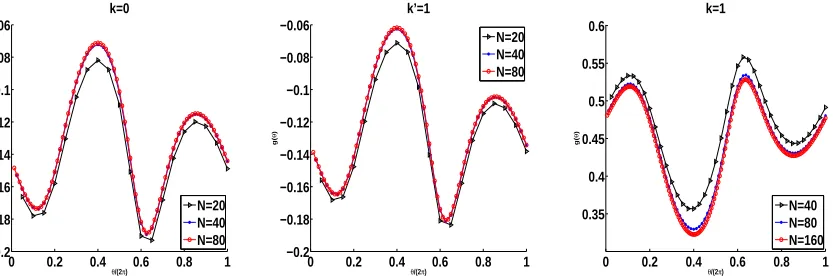
where ∂Gk/∂n is expressed from equation (32). This is shown in figures 7(a)-(c) for k =
0, k′ = 1 and k = 1, for δ = 0.3, R = 1.5 and various degrees of freedom N. From these
figures it can be seen that the numerical results are convergent, as the number of degrees of freedom increases. Twenty, respectively forty evenly spread points out of the curves N = 40 (for k= 0 and k′ = 1), respectively, N = 80 (for k= 1) are chosen as Neumann numerically
simulated data (8) in the inverse problem which is solved using N = 20 (for k = 0 and
k′ = 1), respectively, N = 40 (for k = 1).
0 0.2 0.4 0.6 0.8 1 −0.2 −0.18 −0.16 −0.14 −0.12 −0.1 −0.08 −0.06 k=0
θ/(2π)
g( θ ) N=20 N=40 N=80
0 0.2 0.4 0.6 0.8 1 −0.2 −0.18 −0.16 −0.14 −0.12 −0.1 −0.08 −0.06 k’=1
θ/(2π)
g( θ ) N=20 N=40 N=80
0 0.2 0.4 0.6 0.8 1 0.35 0.4 0.45 0.5 0.55 0.6 k=1
θ/(2π)
[image:17.612.91.508.333.472.2]g( θ ) N=40 N=80 N=160
Figure 7: The normal derivative (8) obtained by solving the direct problem (9), (12), (16), (17) and (70) using the MFS with various values of N for k = 0, k′ = 1 andk = 1.
iter=100 iter=500 iter=1000
[image:18.612.109.492.28.273.2]iter=1500 iter=2000 iter=4000
Figure 8: The reconstructed inner source domain for various numbers of iterations for p = 10% noise and no regularization, for example 2(a) withk = 0.
λ1=λ
2=10
−9 λ
1=λ2=10 −6
λ1=λ
2=10
−5 λ
1=λ2=10 −4
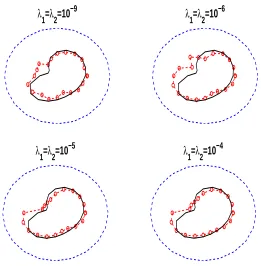
[image:18.612.170.431.360.626.2]λ1=λ
2=0 λ1=λ2=10−6
λ1=λ
2=10
−4 λ
[image:19.612.169.430.25.291.2]1=λ2=10 −3
Figure 10: The reconstructed inner source domain after 500 iterations for noisep= 10% and regularization, for example 2(b) with k′ = 1.
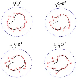
λ1=λ
2=0 λ1=λ2=10−9
λ1=λ
2=10
−8 λ
1=λ2=10 −7
[image:19.612.170.431.377.643.2]5
Conclusions
In this paper, an inverse geometric problem which consists of reconstructing the unknown support of a source in the Poisson equation from a single pair of exterior boundary Cauchy data has been investigated using the MFS. Several examples have been investigated showing that the numerical results are satisfactory reconstructions for the unknown support of a source domain with reasonable stability against inverting noisy data. Regularization method has been used in order to obtain stable and accurate numerical results. Extensions to three-dimensional and time-dependent problems, see Harbrecht and Tausch (2011), will be the subject of a future work.
6
Acknowledgements
The authors extend their appreciation to the Deanship of Scientific Research at King Saud University for funding this work through research group no RG-1437-019.
References
1. C.J.S. Alves and C.S. Chen (2005) A new method of fundamental solutions applied to nonhomogeneous elliptic problems, Advances in Computational Mathematics 23, 125-142.
2. C.J.S. Alves, N.F.M. Martins and N.C. Roberty (2009) Full identification of acoustic sources with multiple frequencies and boundary measurements, Inverse Problems and Imaging 3, 275-294.
3. K.E. Atkinson (1985) The numerical evaluation of particular solutions for Poisson’s equation, IMA Journal of Numerical Analysis5, 319-338.
4. A.H. Barnett and T. Betcke (2008) Stability and convergence of the method of funda-mental solutions for Helmholtz problems on analytic domains,Journal of Computational Physics 227, 7003-7026.
5. M. Belge, M. Kilmer and E.L. Miller (2002) Efficient determination of multiple
regular-ization parameters in a generalized L-curve framework, Inverse Problems18, 1161-1183.
6. J.R. Berger and A. Karageorghis (1999) The method of fundamental solutions for heat conduction in layered materials, International Journal for Numerical Methods in Engi-neering 45, 1681-1694.
7. B. Bin-Mohsin and D. Lesnic (2011) The method of fundamental solutions for Helmholtz-type equations in composite materials, Computers and Mathematics with Applications 62, 4377-4390.
9. A. Bogomolny (1985) Fundamental solutions method for elliptic boundary value prob-lems, SIAM Journal on Numerical Analysis 22, 644-669.
10. A. Canelas, A. Laurain and A.A. Novotny (2014) A new reconstruction method for the inverse potential problem, Journal of Computational Physics 268, 417-431.
11. W. Chen and Y.C. Hon (2003) Numerical investigation on convergence of boundary knot method in the analysis of homogeneous Helmholtz, modified Helmholtz, and convection-diffusion problems, Computer Methods in Applied Mechanics and Engineering 192, 1859-1875.
12. Z. Chen, Y. Lu, Y. Xu and H. Yang (2008) Multi-parameter Tikhonov regularization for linear ill-posed operator equations, Journal of Computational Mathematics 26, 37-55.
13. A. El-Badia and T. Ha-Duong (2000) An inverse source problem in potential analysis,
Inverse Problems 16, 651-663.
14. R. Ennenbach and H. Niemeyer (1996) The inclusion of Dirichlet eigenvalues with sin-gularity functions, ZAMM 76, 377-383.
15. H. Harbrecht and J. Tausch (2011) An efficient numerical method for a shape identifi-cation problem arising from the heat equation, Inverse Problems27, 065013 (18 pages).
16. F. Hettlich and W. Rundell (1996) Iterative methods for the reconstruction of an inverse potential problem, Inverse Problems 12, 251-266.
17. M. Ikehata (1999) Reconstruction of a source domain from the Cauchy data, Inverse Problems 15, 637-643.
18. V. Isakov (1990) Inverse Source Problems, Mathematical Surveys and Monographs, Vol.34, Providence, RI, American Mathematical Society.
19. V. Isakov (2006)Inverse Problems for Partial Differential Equations, 2nd edn., Springer, New York.
21. V. Isakov, S. Leung and J. Qian (2011) A fast local level set method for inverse gravime-try, Communications in Computational Physics 10, 1044-1070.
22. K. Ito and J.-C. Liu (2013) Recovery of inclusions in 2D and 3D domains for Poisson’s equation, Inverse Problems 29, 075005 (19 pages).
23. O. Ivanyshyn and R. Kress (2006) Nonlinear integral equations for solving inverse bound-ary value problems for inclusions and cracks, Journal of Integral Equations and Appli-cations 18, 13-38.
24. B. Jin and Y. Zheng (2005) Boundary knot method for some inverse problems asso-ciated with the Helmhholtz equation, International Journal for Numerical Methods in Engineering 62, 1636-1651.
26. M. Jourhmane (1993) Methodes Numeriques de Resolution d’un Probleme d’Electroencephalographie, PhD Thesis, Universite de Rennes I, France.
27. A. Karageorghis and D. Lesnic (2009) Detection of cavities using the method of funda-mental solutions, Inverse Problems in Science and Engineering17, 803-820.
28. A. Karageorghis, D. Lesnic and L. Marin (2011) The MFS for inverse geometric problems, Inverse Problems and Computational Mechanics, Vol.1, (eds. L. Marin, L. Munteanu and V. Chiroiu), Editura Academiei, Bucharest, Romania, Chapter 8, pp.191-216.
29. A. Karageorghis, D. Lesnic and L. Marin (2013) A moving pseudo-boundary MFS for three-dimensional void detection, Advances in Applied Mathematics and Mechanics 5, 510-527.
30. D. Lesnic and B. Bin-Mohsin (2012) Inverse shape and surface heat transfer coefficient identification, Journal of Computational and Applied Mathematics 236, 1876-1891.
31. R.G.S. Mamud, N.C. Roberty and C.J.S. Alves (2014) Analytical observability of sym-metric star shaped sources for modified Helmholtz model, 8th International Conference on Inverse Problems in Engineering, May 12-15, 2014, Poland, (eds. I. Szczygiel, A.J. Nowak and M. Rojczyk), pp.179-188.
32. N.F.M. Martins (2012) An iterative shape reconstruction of source functions in potential problem using the MFS, Inverse Problems in Science and Engineering20, 1175-1193.