The Hi-GAL compact source catalogue – I. The physical properties of the clumps in the inner Galaxy (−71⋅º 0 < ℓ < 67⋅º 0)

Advance Access publication 2017 June 15

The Hi-GAL compact source catalogue – I. The physical properties of the

clumps in the inner Galaxy (

−

71

.

◦

0

< <

67

◦

.

0)

Davide Elia,

S. Molinari,

E. Schisano,

M. Pestalozzi,

S. Pezzuto,

M. Merello,

A. Noriega-Crespo,

T. J. T. Moore,

D. Russeil,

J. C. Mottram,

R. Paladini,

F. Strafella,

M. Benedettini,

J. P. Bernard,

A. Di Giorgio,

D. J. Eden,

Y. Fukui,

R. Plume,

J. Bally,

P. G. Martin,

S. E. Ragan,

S. E. Jaffa,

F. Motte,

L. Olmi,

N. Schneider,

L. Testi,

F. Wyrowski,

A. Zavagno,

L. Calzoletti,

F. Faustini,

P. Natoli,

P. Palmeirim,

F. Piacentini,

L. Piazzo,

G. L. Pilbratt,

D. Polychroni,

A. Baldeschi,

M. T. Beltr´an,

N. Billot,

L. Cambr´esy,

R. Cesaroni,

P. Garc´ıa-Lario,

M. G. Hoare,

M. Huang,

G. Joncas,

S. J. Liu,

B. M. T. Maiolo,

K. A. Marsh,

Y. Maruccia,

P. M`ege,

N. Peretto,

K. L. J. Rygl,

P. Schilke,

M. A. Thompson,

A. Traficante,

G. Umana,

M. Veneziani,

D. Ward-Thompson,

A. P. Whitworth,

H. Arab,

M. Bandieramonte,

U. Becciani,

M. Brescia,

C. Buemi,

F. Bufano,

R. Butora,

S. Cavuoti,

A. Costa,

E. Fiorellino,

A. Hajnal,

T. Hayakawa,

P. Kacsuk,

P. Leto,

G. Li Causi,

N. Marchili,

S. Martinavarro-Armengol,

A. Mercurio,

M. Molinaro,

G. Riccio,

H. Sano,

E. Sciacca,

K. Tachihara,

K. Torii,

C. Trigilio,

F. Vitello

and H. Yamamoto

Accepted 2017 May 31. Received 2017 May 25; in original form 2016 September 15

A B S T R A C T

Hi-GAL (Herschel InfraRed Galactic Plane Survey) is a large-scale survey of the Galactic plane, performed withHerschelin five infrared continuum bands between 70 and 500µm. We present a band-merged catalogue of spatially matched sources and their properties derived from fits to the spectral energy distributions (SEDs) and heliocentric distances, based on the photometric catalogues presented in Molinari et al., covering the portion of Galactic plane

−71◦.0 < <67◦.0. The band-merged catalogue contains 100 922 sources with a regular SED, 24 584 of which show a 70-µm counterpart and are thus considered protostellar, while the remainder are considered starless. Thanks to this huge number of sources, we are able to carry out a preliminary analysis of early stages of star formation, identifying the conditions that characterize different evolutionary phases on a statistically significant basis. We calculate surface densities to investigate the gravitational stability of clumps and their potential to form massive stars. We also explore evolutionary status metrics such as the dust temperature, luminosity and bolometric temperature, finding that these are higher in protostellar sources compared to pre-stellar ones. The surface density of sources follows an increasing trend as they evolve from pre-stellar to protostellar, but then it is found to decrease again in the majority of the most evolved clumps. Finally, we study the physical parameters of sources with respect

Properties of Hi-GAL clumps in the inner Galaxy

101

to Galactic longitude and the association with spiral arms, finding only minor or no differences between the average evolutionary status of sources in the fourth and first Galactic quadrants, or between ‘on-arm’ and ‘interarm’ positions.

Key words: catalogues – ISM: clouds – dust, extinction – local interstellar matter – infrared:

ISM – submillimetre: ISM.

1 I N T R O D U C T I O N

The formation of stars remains one of the most important unsolved problems in modern astrophysics. In particular, it is not clear how massive stars (M>8 M) form, despite their importance in the evolution of the Galactic ecosystem (e.g. Ferri`ere2001; Bally & Zinnecker2005). The formation of high-mass stars is not as well-understood as that of low-mass stars, mainly because of a lack of observational facts upon which models can be built. High-mass stars are intrinsically difficult to observe because of their low num-ber in the Galaxy, their large distance from the Sun and their rapid evolution. Numerous observational surveys have been undertaken in recent years in different wavebands to obtain better statistics on massive pre-stellar and protostellar objects. (Jackson et al.2006; Stil et al.2006; Lawrence et al.2007; Carey et al.2009; Church-well et al.2009; Schuller et al. 2009; Rosolowsky et al. 2010; Hoare et al.2012; Urquhart et al.2014a; Moore et al.2015). Among these, Hi-GAL (Herschel InfraRed Galactic Plane Survey) is the only complete far-infrared (FIR) survey of the Galactic plane.

Hi-GAL (Molinari et al.2010a) is an Open Time Key Project, which was granted about 1000 h of observing time using the

Herschel Space Observatory (Pilbratt et al. 2010). It delivers a complete and homogeneous survey of the Galactic plane in five continuum FIR bands between 70 and 500µm. This wavelength coverage allows us to trace the peak of emission of most of the cold (T<20 K) dust in the Milky Way at high resolution for the first time, material that is expected to trace the early stages of the formation of stars across the mass spectrum. Hi-GAL data were taken using in parallel two of the three instruments aboardHerschel, PACS (70-and 160-µm bands, Poglitsch et al.2010) and SPIRE (250-, 350-and 500-µm bands, Griffin et al.2010).

This paper is meant to complete the discussions presented in Molinari et al. (2016a) on the construction of the photometric cata-logue for the portion of Galaxy in the range−71.◦067◦.0,|b| <1.◦0, an area corresponding to the first Hi-GAL proposal (subse-quently extended to the whole Galactic plane). In particular, here we explain how we went from the photometric catalogue to the physical one, introducing band-merging, searching for counterparts, assign-ing distances as well as constructassign-ing and fittassign-ing spectral energy distributions (SEDs). In the last part of this paper, in which the distribution of sources with respect to their position in the Galactic plane is analysed in detail, we focus on two regions, i.e. 289.◦0< <340◦_.0 and 33◦_.0_{< <}67◦_.0. The innermost part of the Galactic plane, including the Galactic Centre, where the kinematic distance estimate is particularly problematic, will be discussed in a separated paper (Bally et al., in preparation), while the two longitude ranges containing the two tips of the Galactic bar (340◦.0< <350.◦0 and 19◦.0< <33◦.0) have been presented in Veneziani et al. (2017).

1.1 Brief presentation of the surveyed regions

1.1.1 Fourth Galactic quadrant

In the longitude range investigated in more detail in this paper, three spiral arms are in view (see Fig.1), according to a four-armed spiral model of the Milky Way (Urquhart et al.2014a, and references

therein). Moving towards the Galactic Centre, for 289◦ 310◦the Carina–Sagittarius arm is observed, while at∼310◦the tangent point of the Scutum–Crux arm is encountered (Garc´ıa et al.

2014). The emission from this latter arm is expected to dominate up to the tangent point of the Norma arm at ∼ 330◦. Around this longitude, the main peak of the OB star formation distribution across the Galaxy is found (Bronfman et al. 2000). Finally, the tangent point of the subsequent arm, the so-called3-kpcarm, is located at∼338◦(Garc´ıa et al.2014), i.e. very close to the inner limit of the investigated zone.

Significant star formation activity is found in the surveyed region, as testified by the presence of 103 out of 481 star-forming complexes in the list of Russeil (2003), and of 393 star-forming regions out of 1735 in the Avedisova (2000) overall catalogue, of which 29 are Hα-emission regions of the RCW catalogue (Rodgers, Campbell & Whiteoak1960). Furthermore, 337 out of 1449 regions with embedded OB stars of the Bronfman, Nyman & May (1996) and Bronfman et al. (2000) list are found in this region of the sky.

Hi-GAL observations of the fourth Galactic quadrant have al-ready been used for studying InfraRed Dark Clouds (IRDCs, Egan et al.1998) in the 300◦30◦,|b| ≤1◦range (Wilcock et al.

2012a,b), highlighting the fundamental role of the HerschelFIR data for exploring the internal structure of these candidate sites for massive star formation. Furthermore, Veneziani et al. (2017) used the catalogue presented here to study the compact source population in the far tip of the long Galactic bar. These data will be exploited, if needed, in this article as well, for instance, for comparison between the fields studied in this paper and inner regions of the Galaxy.

Finally, the nearby Coalsack nebula (d=100–200 pc, see refer-ences in Beuther et al.2011) is also seen in the foreground of our field (300◦ 307◦, Wang et al.2013). It is one of the most prominent dark clouds in the southern Milky Way but shows no ev-idence of recent star formation (e.g. Kato et al.1999; Kainulainen et al.2009).

1.1.2 First Galactic quadrant

In the first quadrant portion investigated in more detail in this paper (33◦67◦), two spiral arms are in view, namely the Carina– Sagittarius and the Perseus arms. The Carina–Sagittarius tangent point is found at51◦(Vall´ee2008) near the W51 star-forming region. From here to the endpoint of the region we are considering, only the Perseus arm is expected.

This area is smaller than that surveyed in the fourth quadrant and has a lower rate of star formation activity per unit area. Russeil (2003) finds 33 star-forming regions in this area, and Avedisova (2000) finds just 97.

Figure 1. Plot of the position in the Galactic plane of the pre-stellar (red dots) and protostellar (blue dots) Hi-GAL objects provided with a distance estimate. Unbound objects are not shown to reduce the crowding of the plot. For definitions of pre-stellar, protostellar and unbound objects, see Section 3.5. Two pairs of black solid lines delimit the longitude ranges analysed in this paper. Further sources are found closer to the Galactic Centre, most of which are analysed in Veneziani et al. (2017, see their fig. 1). In the inner zone devoid of points, distances were not estimated (see text); thus, only distance-independent source properties were derived. The Galactic Centre is indicated with a×symbol at coordinates [x,y]=[0, 0] and the Sun with an orange dot at coordinates [0, 8.5], at the bottom of the plot. Cyan dashed lines indicate the Galactic longitude in steps of 30◦.Rdenote Galactocentric distances (light-green dashed circles) and

ddenote heliocentric ones (grey dotted circles), with the following steps: 1, 5 and 10 kpc. Spiral arms, from the four-arm Milky Way prescription of Hou, Han & Shi (2009), are plotted with different colours, with the arc–colour correspondence reported in the upper left-hand corner of the plot. In particular, the Norma arm is represented using two colours: magenta for the inner part of the arm and brown for the portion of it generally designated as the outer arm, which starting point is established by comparison with Momany et al. (2006). Finally, the local arm, not included in the model of Hou et al. (2009), is drawn, taken from Xu et al. (2016).

2011) and diffuse emission morphology (Martin et al.2010). As in the case of the fourth quadrant, the catalogue presented here has already been used by Veneziani et al. (2017) for studying the clump population at the near tip of the Galactic bar. Finally, a recent paper of Eden et al. (2015) focused on two lines of sight centred towards =30◦and 40◦, studying arm/interarm differences in luminosity distribution of Hi-GAL sources.

1.2 Structure of this paper

This paper is organized as follows. In Section 2, the data reduc-tion, source detection and photometry strategy are briefly presented,

Properties of Hi-GAL clumps in the inner Galaxy

103

the behaviour of arm versus interarm sources is briefly discussed. Further details on how the catalogue is organized, and on possible biases affecting the listed quantities, are provided in the appendices at the end of this paper.

2 DATA : M A P M A K I N G A N D C O M PAC T S O U R C E E X T R AC T I O N

The technical features of the Hi-GAL survey are presented in Molinari et al. (2010a); therefore, here we limit ourselves to a summary of only the most relevant aspects. The Galactic plane was divided into 2×2 deg2_{sections, called ‘tiles’, that were observed}

withHerschelat a scan speed of 60 arcsec s−1_{in two orthogonal}

directions. PACS and SPIRE were used in ‘parallel mode’, i.e. data were taken simultaneously with both instruments (and therefore at all five bands). Note that when used in parallel mode, PACS and SPIRE observe a slightly different region of sky. A more complete coverage is nevertheless recovered when considering contiguous tiles; remaining areas of the sky covered only by either one of the two are not considered for science in this paper. Single maps of the Hi-GAL tiles were obtained from PACS/SPIRE detector timelines using a pipeline specifically developed for Hi-GAL and contain-ing the ROMAGAL map-makcontain-ing algorithm (Traficante et al.2011) and the WGLS post-processing (Piazzo et al.2012) for removing artefacts in the maps.

Astrometric consistency with Spitzer MIPSGAL 24-µm data (Carey et al.2009,http://mipsgal.ipac.caltech.edu/) is obtained by applying a rigid shift to the entire mosaic. This is obtained as the mean shift measured on a number of bright and isolated sources common toSpitzer24-µm and Hi-GAL PACS 70-µm data.

The further astrometric registration of SPIRE maps is then carried out by repeating the same procedure, but comparing counterparts of the same source at 160 and 250µm.

Compact sources were detected and extracted using the algorithm CUTEX(Molinari et al.2011), which is based on the study of the

curvature of the images. This is done by calculating the second derivative at any pixel of the Hi-GAL images, efficiently damping all emission varying on intermediate to large spatial scales, and am-plifying emission concentrated in small scales. This principle is par-ticularly advantageous when extracting sources that appear within a bright and highly variable background emission. The final inte-grated fluxes are then estimated by CUTEXthrough a bi-dimensional Gaussian fit to the source profile. All details of the photometric cat-alogue are presented by Molinari et al. (2016a), who also report estimates of the completeness limits in flux in each band, measured by extracting a controlled 90 per cent sample of sources artificially spread on a representative sample of real images. Such limits in the regions investigated in this paper are discussed in Appendix C2 for their implications on the estimate of source mass completeness limits as a function of the heliocentric distance.

The final version of the single-band catalogues of the portion of Hi-GAL data presented here contains 123 210, 308 509, 280 685, 160 972 and 85 460 entries in the 70-, 160-, 250-, 350- and 500-µm bands, respectively.

3 F R O M P H OT O M E T RY T O P H Y S I C S

This paper focuses on the study of compact cold objects extracted fromHerscheldata. Within this framework, a final catalogue of ob-jects for scientific studies has been obtained by merging the Hi-GAL single-band photometric catalogues and filtering the resulting five-band catalogue, applying specific constraints to the source SEDs. In

the following sections, the steps of these processes are explained in detail: band-merging, search for counterparts beyond theHerschel

frequency coverage, assigning distances, SED filtering and fitting.

3.1 Band-merging and source selection

The first step for creating a multiwavelength catalogue consists of assigning counterparts of a given source acrossHerschelbands. This operation is based on iterating a positional matching (cf. Elia et al.

2010,2013) between source lists obtained at two adjacent bands. In this paper, however, instead of assuming a fixed matching radius as done in previous works, the matching region consisted of the ellipse describing the source at the longer of the two wavelengths.1

In other words, a source has a counterpart at shorter wavelength if the centroid of the latter falls within the ellipse fitted to the former. In this way, it is possible that more than one counterpart fall into the longer wavelength ellipse. In such multiplicity cases, the association is established only with the short-wavelength counterpart closest to the long-wavelength ellipse centroid.2_{The remaining ones are}

reported as independent catalogue entries, and considered for further possible counterpart search at shorter wavelengths. At the end of the five band-merging, a catalogue is produced, in which each entry can contain from one to five detections in as many bands.

The subsequent step is to filter the obtained five-band catalogue in order to identify SEDs that are eligible for the modified blackbody (hereafter grey body) fit, hence to derive the physical properties of the objects. This selection is based on considerations of the regularity of the SEDs in the range 160–500µm, since the 70-µm band is generally expected to depart from the grey-body behaviour (e.g. Bontemps et al.2010; Schneider et al.2012).

First of all, as done in Elia et al. (2013), only sources belonging to the common PACS+SPIRE area and detected at least in three consecutiveHerschel bands (i.e. the combinations 160–250–350

µm or 250–350–500µm or, obviously, 160–250–350–500µm) were selected.

Secondly, fluxes at 350 and 500µm were scaled according to the ratio of deconvolved source linear sizes, taking as a reference the size at 250µm (cf. Motte et al.2010a; Nguyen Luong et al.2011). This choice is supported by the fact that cold dust is expected to have significant emission around 250µm; also, according to the adopted constraints to filter the SEDs, this is the shortest wavelength in common for all the selected SEDs. Finally, we searched for further irregularities in the SEDs such as dips in the middle, or peaks at 500µm.

At the end of the filtering pipeline, we remain with 100 922 sources. For each of these sources, we estimate physical parame-ters such as dust temperature, surface density and, when distance is available, linear size, mass and luminosity, by fitting a single-temperature grey body to the SED. The details of this procedure are described in Section 4. Clearly, the determination of source physical quantities such as temperature and mass is more reliable when a bet-ter coverage of the SED is available. Based on the selection cribet-teria listed above, sources in our catalogue can be confirmed, even con-sidering the 70-µm flux, with detections at only three bands: This is the case for combinations 160–250–350µm (with no detection at 70µm) and 250–350–500µm (that we call ‘SPIRE-only’ sources),

1_{Such ellipse corresponds to the half-height section of the two-dimensional}

Gaussian fitted by CUTEXto the source profile.

2_{For the 70-µm band, we also take into account possible multiplicity for}

Table 1. Number of sources in the Hi-GAL catalogue, in ranges of longitude.

Longitude range Protostellar Highly reliable starless (pre-stellar) Poorly reliable starless (pre-stellar) Total w/ distance w/o distance w/ distance w/o distance w/ distance w/o distance

−71◦≤ <−20◦ 8227 1425 10 384 (9598) 2978 (2265) 10 696 (7531) 3321 (1519) 37 031

−20◦≤ <−10◦ 1752 273 2667 (2506) 611 (537) 2548 (1855) 591 (345) 8442

−10◦≤ <0◦ 0 2154 0 (0) 3357 (3139) 0 (0) 3417 (2544) 8928 0◦≤ <19◦ 505 3165 398 (380) 5689 (5271) 318 (249) 5488 (4053) 15 563 19◦≤ <33◦ 2646 549 3172 (2893) 1260 (1068) 3045 (2200) 1312 (832) 11 984 33◦≤ <67◦ 2704 1184 4189 (3818) 3149 (2548) 3814 (2520) 3934 (2000) 18 974

Total 15 834 8750 20 810 (19 195) 17 044 (14 828) 20 421 (14 355) 18 063 (11 293) 100 922

which we consider as genuine SEDs, although more affected by a less reliable fit (especially the SPIRE-only case, in which it might be difficult to constrain the SED peak, and consequently the tem-perature). For this reason, after the SED filtering procedure, we further split our SEDs into two sub-catalogues: ‘high reliability’ (62 438 sources) and ‘low reliability’ (38 484 sources). Notice that, according to the definitions that will be provided in Section 3.5, all the sources in the latter list belong to the class of ‘starless’ compact sources.

In Table1, the source number statistics for the band-merged cata-logue are provided, divided in ranges of longitude (identified by the two intervals studied by Veneziani et al.2017) and in evolutionary stages introduced in Section 3.5.

3.2 Caveats on SED building and selection

Building a five-band catalogue and selecting reliable sources for scientific analysis require a set of choices and assumptions, which have been described in the previous sections. Here we collect and explicitly recall all of them to focus the reader’s attention on the lim-itations that must be kept in mind when using the Hi-GAL physical catalogue:

(i) The concept of ‘compact source’ used for this catalogue refers to unresolved or poorly resolved structures, whose size, therefore, does not exceed a few instrumental PSFs ( 3, Molinari et al.

2016a). Structures with larger angular sizes – such as a bright diffuse interstellar medium (ISM), filaments or bubbles – escape from this definition and are not considered in the present catalogue.

(ii) The appearance of the sky varies strongly throughout the wavelength range covered byHerschel. The lack of a detection in a given band may be ascribed to a detection error, or to the physical conditions of the source as, for instance, the case of a warm source seen by PACS but undetectable at the SPIRE wavelengths. In this respect, the present catalogue does not aim to describe all star formation activity within the survey area, but rather to provide a census of the coldest compact structures, corresponding to early evolutionary stages in which internal star formation activity has not yet been able to dissipate the dust envelope, or has not started at all. Detections at 70µm only, or at 70/160µm, or at 70/160/250µm, are expected to have counterparts in the mid-IR (MIR); such cases, corresponding to more evolved objects, surely deserve to be further studied, but this lies out of the aims of this paper and is reserved for future works.

(iii) The band-merging procedure works fine in the ideal case of a source detected at all wavelengths as a bright and isolated peak. Possible multiplicities, however, can produce multiple branches in the counterpart association, so that, for instance, the flux at a given wavelength might result from the contributions of two or more coun-terparts detected separately at shorter wavelengths. This can also

introduce inconsistent fluxes in the SEDs and produce irregularities such that several bright sources present in the Hi-GAL maps might be ruled out from the final catalogue according to the constraints described in Section 3.1.

(iv) Very bright sources might be ruled out by the filtering al-gorithm due to saturation occurring at one or more bands, which produces unrecoverable gaps in the SEDs.

(v) The physical properties derived fromHerschelSED analysis (see next sections) are global (e.g. mass, luminosity) or average (e.g. temperature) quantities for sources that, depending on their distance, can be characterized by a certain degree of internal but unresolved structure (see Section 6.1), as will be discussed in Appendix C.

3.3 Counterparts at non-Herschelwavelengths

For every entry in the band-merged filtered catalogue, we searched for counterparts at 24µm (MIPSGAL, Gutermuth & Heyer2015) as well as at 21µm (MSX, Egan et al.2003) and 22µm (WISE, Wright et al. 2010). The fluxes of these counterparts, typically associated with a warm internal component of the clump, are not considered for subsequent grey-body fitting of the portion of the SED associated with cold dust emission, but only for estimating the source bolometric luminosity.

In particular, we notice that the choice of sources in the cat-alogue of Gutermuth & Heyer (2015) is rather conservative, and only a small fraction hasF24<0.005 Jy. For this reason, we

per-formed an additional search of sources in the MIPSGAL maps, using theAPEXsource extractor3_{(Makovoz & Marleau2005), in}

order to recover those sources that, from a visual inspection of the maps, appear to be real, although for some reason were not included in the original catalogue. Furthermore, as a cross-check, a similar procedure has been performed also withDAOFIND (Stetson1987),

and only sources confirmed by this have been added to the photom-etry list of Gutermuth & Heyer (2015). Following this procedure, approximately 2000 additional SEDs have been complemented with a flux at 24µm, mostly having fluxes in the range 0.0001<F24<

0.001 Jy. The risk of adding poorly reliable sources with low signal-to-noise ratio is mitigated by the fact that 24-µm counterparts of ourHerschelsources are considered for scientific analysis only if they are confirmed by a detection at 70µm (see Section 3.5 and Appendix B).

To assign counterparts to the Hi-GAL sources at 21, 22 and 24

µm, the ellipse representing the source at 250µm was used as the matching region, and the flux of all counterparts at a given wave-length within this region was summed up into one value. Indeed,

3_{http://irsa.ipac.caltech.edu/data/SPITZER/docs/dataanalysistools/}

Properties of Hi-GAL clumps in the inner Galaxy

105

possible occurrences of multiplicity can induce a relevant contri-bution at MIR wavelengths in the calculation of the bolometric luminosity of Hi-GAL sources.

On the long-wavelength side of the SED, we cross-matched our band-merged and filtered catalogue with those of Csengeri et al. (2014) from the ATLASGAL survey (870µm, Schuller et al.2009) and of Ginsburg et al. (2013) from the BOLOCAM Galactic Plane Survey (BGPS, 1.1 mm, Rosolowsky et al.2010; Aguirre et al.

2011). The adopted searching radius was 19 arcsec for the former and 33 arcsec for the latter, corresponding to the full width at half-maximum of the instruments at the observed wavelengths. Out of 10 861 entries in the ATLASGAL catalogue, 10 517 of them lie inside the PACS+SPIRE common science area considered in this paper, of which 6136 are found to be associated with a source of our catalogue through this 1:1 matching strategy. Similarly, 6020 out of 8594 entries of the BGPS catalogue lie in the common science area, of which 4618 turn out to be associated with an entry of our catalogue. Finally, access to ATLASGAL images allowed us to extract further counterparts, not reported in the list of Csengeri et al. (2014), by using CUTEX. In cases in which the deconvolved

size of the ATLASGAL and/or BGPS counterpart is larger than the one measured at 250µm, fluxes were rescaled according to the procedure described in Section 3.1.

3.4 Distance determination

Assigning distances to sources is a crucial step in the process of giving physical significance to the information extracted from Hi-GAL data. While reliable distance estimates are available for a limited number of known objects, as, for example, HIIregions

(e.g. Fish et al.2003) or masers (e.g. Green & McClure-Griffiths

2011), this information does not exist for the majority of Hi-GAL sources. Therefore, we adopted the scheme presented in Russeil et al. (2011), based on the Galactic rotation model of Brand & Blitz (1993), to assign kinematic distances to a large proportion of sources: A12_{CO (or}13_{CO) spectrum is extracted at the line of}

sight of every Hi-GAL source, and the velocity of the local stan-dard of restVLSRof the brightest spectral component is assigned to

it, allowing the calculation of a kinematic distance. To determine theVLSR, the13CO data from the Five College Radio Astronomy

Observatory (FCRAO) Galactic Ring Survey (GRS, Jackson et al.

2006), and12_{CO and}13_{CO data from the Exeter-FCRAO Survey}

(Brunt et al., in preparation; Mottram et al., in preparation) were used for the portion of Hi-GAL covering the first Galactic quadrant for <55◦and for >55◦, respectively. The pixel size of those CO cubes is 22.5 arcsec, corresponding to Nyquist sampling of the FCRAO beam. NANTEN12_{CO data (Onishi et al.2005) were used}

to assign velocities to Hi-GAL sources in the fourth quadrant. The pixel size of these data is 4 arcmin (against an angular resolution of 2.6 arcmin), so that more than one Hi-GAL source might fall on to the same CO line of sight, and the same distance is assigned to them. The spectral resolutions of the two data sets were 0.15 and 1.0 km s−1_{, respectively.}

Once theVLSRis determined, the near/far distance ambiguity is

solved by matching the source positions with a catalogue of sources with known distances (HII regions, masers and others) or,

alter-natively, with features in extinction maps (in this case, the near distance is assigned). In cases for which none of the aforemen-tioned data can be used, the ambiguity is always arbitrarily solved in favour of the far distance, and a ‘bad-quality’ flag is given to that assignment.

The additional use of extinction maps to solve for distance am-biguity (Russeil et al.2011) (where applicable) can be a source of error, whose magnitude typically increases with increasing dif-ference between the near and far heliocentric distance solutions. For this paper, we rely on the use of extinction maps for practical reasons and also because, for most of the sources, no spectral line emission has yet been observed other than what can be extracted from the two CO surveys.

Finally, at present, no distance estimates have been obtained in the longitude range−10◦_.2_{< <}14◦_.0, due to the difficulty in estimating the kinematic distances of sources in the direction of the Galactic Centre. We were able to assign a heliocentric distance to 57 065 sources out of the 100 922 of the band-merged filtered catalogue, i.e. 56 per cent (see also Table1). However, for 35 904 of these, the near/far ambiguity has not been solved, since the extinction information is not available, and the far distance is assigned by default (see above).

The distribution of sources in the Galactic plane is shown in Fig.1. It can be seen that the available distances do not produce a clear segregation between high-source-density regions corresponding to spiral arm locations and less populated interarm regions, as will be discussed in more detail in Section 8.2. On one hand, massive star-forming clumps are expected to be organized along spiral arms (e.g. CH3OH and H2O masers observed by Xu et al.2016), while, on the

other hand, the large number of sources present in our catalogue, corresponding to a large variety of physical and evolutionary condi-tions probed withHerschel, makes it likely to also include clumps located outside the arms. Any consideration of this aspect is subject to a more correct estimate of heliocentric distances: The work of assigning distances to Hi-GAL sources is still in progress within the VIALACTEA project, and a more refined set of distances (and for an increased number of sources) will be delivered in Russeil et al. (in preparation).

3.5 Starless and protostellar objects

One of the most important steps in the determination of the evolutionary stages of Hi-GAL sources is discriminating between pre-stellar and protostellar sources, namely starless but gravita-tionally bound objects and objects showing signatures of ongoing star formation, respectively. Here we follow the approach already described in Elia et al. (2013). If a 70-µm counterpart is available, that object can with a high degree of confidence be labelled as protostellar (Dunham et al.2008; Ragan, Henning & Beuther2013; Svoboda et al.2016). This criterion works well for relatively nearby objects, but as soon as we extend our studies to regions farther away than, say, 4–5 kpc, two competing effects concur in confusing the source counts (see also Baldeschi et al.2017), both affecting the estimates of the star formation rate (SFR). First, at large distances, 70-µm counterparts of relatively low mass sources might be missed (and sources mislabelled) because of limits in sensitivity.4

Secondly, since the protostellar label is given on the basis of the detection of a 70-µm counterpart, starless and protostellar cores close together and far away could be seen and labelled as a single

4_{For example, applying equation (4) (presented in the following), a grey}

body with a mass of 50 M, temperature of 15 K, dust emissivity with exponentβ=2 with the same reference opacity as adopted in this paper (see Section 4) and located at a distance of 10 kpc would have a flux of 0.02 Jy at 70µm, and of 0.84 Jy at 250µm, consequently detectable with

Figure 2. Multiwavelength 2×2 arcmin2_{images of two sources listed in our catalogue, to provide an example of a protostellar (upper 11 panels) and a}

pre-stellar source (lower 11 panels). The source coordinates and physical properties are reported above each set of panels. For each source position, 10 images at 21, 22, 24, 70, 160, 250, 350, 500, 870 and 1100µm, taken from the survey indicated in the title, are shown (the colour scale is logarithmic, in arbitrary units). Finally, the SED of each of the two sources is shown: filled and open symbols indicate fluxes that are taken into account or not, respectively, for the grey-body fit (solid line, see Section 4). The grey-shaded area is a geometric representation of the integral calculated to estimate the source bolometric luminosity (see Sections 3.3 and 4).

protostellar clump due to lack of resolution. We address this issue in Appendix C1.

To mitigate the first effect, we performed deeper, targeted ex-tractions at PACS wavelengths towards two types of sources. One type consisted of ‘SPIRE-only’ sources, i.e. sources clearly detected only at 250, 350 and 500µm. Since SED fitting for such sources is poorly constrained, a further extraction at 160µm, deeper than that of Molinari et al. (2016a), was required in order to set at least an upper limit for the flux shortwards of what could be the peak of the SED. In this way, 9705 further detections and 9992 upper limits at 160µm were recovered.

The second type of sources consists of those showing a 160-µm counterpart (original or found after a deeper search) but no detection at 70µm. To ascertain that the starless nature of these objects is not assigned simply due to a failure of the source-detection process, we performed a deeper search for a 70-µm counterpart towards those targets: In this way, a possible clear counterpart not originally listed in the single-band catalogues would allow us to label the object

as protostellar. Adopting this strategy, 912 further detections and 76 215 upper limits at 70µm were recovered.

Whereas the protostellar objects are expected to host ongoing star formation, the relation between starless objects and star forma-tion processes must be further examined, since only gravitaforma-tionally bound sources fulfil the conditions for a possible future collapse. Here we use the so-called ‘Larson’s third relation’ to assess if an ob-ject can be considered bound: The condition we impose involves the source mass,M, and radius,r(see Sections 4 and 6), and is formu-lated asM(r)>460 M(r/pc)1.9_{(Larson1981). Masses above this}

Properties of Hi-GAL clumps in the inner Galaxy

107

One of the aims of this paper is to show the amount of informa-tion that can be extracted simply from continuum observainforma-tions in the FIR/sub-mm, combining Hi-GAL data with other surveys in ad-jacent wavelength bands and using spectroscopic data only to obtain kinematic distances. On one hand, for many sources, these data can be complemented with line observations to obtain a more detailed picture, while, on the other hand, Hi-GAL produced an unprece-dentedly large and unbiased catalogue containing many thousands of newly detected cold clumps, for which it is important to provide a first classification. The criteria we provide to separate different populations, although somewhat conventional in theHerschel liter-ature, remain probably too clear-cut and surely affected by biases we introduced in this section and also discussed in the following sections of this paper. Reciprocal contamination of the samples certainly increases overlap of the physical property distributions obtained separately for the different populations, as will be seen in Sections 6 and 7.

4 S E D F I T T I N G

Once the SEDs of all entries in the filtered catalogue are built by assembling the photometric information, as explained above, it is possible to fit a single-grey-body function to itsλ≥160µm portion, and therefore derive the massMand the temperatureTof the cold dust in those objects.

Many details on the use of the grey body to model FIR SEDs have been provided and discussed by Elia & Pezzuto (2016). Here we report only concepts and analytic expressions that are appropriate for this paper. The most complete expression for the grey body explicitly contains the optical depth:

Fν=(1−e−τν)Bν(Td) , (1)

recently used, e.g. in Giannini et al. (2012), whereF_νis the observed flux density at the frequency_ν,B_ν(Td) is the Planck function at the

dust temperatureTdand is the source solid angle in the sky. The

optical depth can be parametrized, in turn, as

τν =(ν/ν0)β, (2)

where the cut-off frequencyν0=c/λ0is such thatτν0=1, andβis the exponent of the power-law dust emissivity at large wavelengths. After constrainingβ=2, as typically adopted also in the Gould Belt (e.g. K¨onyves et al.2015) and HOBYS (e.g. Giannini et al.2012) consortia, and as recommended by Sadavoy et al. (2013), and to be equal to the source area as measured by CUTEXat the reference

wavelength of 250µm (cf. Elia et al. 2013), the free parameters of the fit remainTandλ0. For these parameters, we explored the

ranges 5≤T≤40 K and 5≤λ0≤350µm, respectively.

The clump mass does not appear explicitly in equation (1) but can be derived from

M=d2 /κref

τref, (3)

as shown by Pezzuto et al. (2012), whereκrefandτrefare the opacity

and the optical depth, respectively, estimated at a given reference wavelengthλref. To preserve the compatibility with previous works

based on otherHerschel key-projects (e.g. K¨onyves et al. 2010; Giannini et al.2012), here we decided to adoptκref=0.1 cm2g−1

atλref=300µm (Beckwith et al.1990, already accounting for a

gas-to-dust ratio of 100), whileτrefcan be derived from equation

(2). The choice of_κrefconstitutes a critical point (Deharveng et al. 2012; Martin et al.2012); thus, it is interesting to show how much the mass would change if another estimate ofκrefwere adopted.

The dust opacity at 300µm from the widely used OH5 model (Os-senkopf & Henning1994) isκ300= 0.13 cm2g−1, which would

produce a 30 per cent underestimation of masses with respect to our case. Preibisch et al. (1993) quote κ1300 = 0.005 cm2 g−1,

which, for β = 2, would correspond to κ300 = 0.094 cm2 g−1,

implying an∼6 per cent larger mass. Similarly, the value of Net-terfield et al. (2009),κ250 = 0.16 cm2g−1, would translate into

κ300=0.11 cm2g−1, practically consistent with the value adopted

here. However, further literature values of κ250 quoted by

Net-terfield et al. (2009) in their table 3 span an order of magnitude fromκ250 =0.024 cm2g−1(Draine & Li2007) toκ250 = 0.22–

0.25 cm2_g−1_{(Ossenkopf & Henning1994), which would lead to a}

factor from 6 to 0.6 on the masses calculated in this paper. For very low values ofλ0(i.e. much shorter than the minimum

of the range we consider for the fit, namely 160µm), the grey body has a negligible optical depth at the considered wavelengths, so that equation (1) can be simplified as follows:

Fν= Mκ

ref d2 ν νref β

Bν(Td) (4)

(cf. Elia et al.2010). We note that the estimate of λ0 does not

affect our results significantly when it impliesτ≤0.1 at 160µm. According to equation (2) and forβ=2, we find that the critical value is encountered forλ0∼50.6µm. If the fit procedure using

equation (1) provides aλ0value shorter than that, the fit is repeated

based on equation (4), and the mass and temperature computed in this alternative way are considered as the definitive estimates of these quantities for that source. In Fig. 3, we show how the temperature and mass values obtained through equations (1) (Ttk,

Mtk) and (4) (Ttn,Mtn) appear generally equivalent as long asλ0

(obtained through the former) is much shorter than 160µm (say,λ < 100µm), since both models have extremely low (or zero) opacities at the wavelengths involved in the fit. Quantitatively speaking, the average and standard deviation of theTtk/Ttnratio forλ <160µm

are 1.01 and 0.02, respectively. However, an increasing discrepancy is visible at increasingλ0, highlighting the tendency of equation (4)

to underestimate the temperature and to overestimate the mass. SED fitting is performed byχ2_{optimization of a grey-body model}

on a grid that is refined in successive iterations to converge on the final result. The strategy of generating an SED grid to be compared with data also gives us the advantage of applying PACS colour corrections directly to the model SEDs (since its temperature is known for each of them), rather than correcting the data iteratively (cf. Giannini et al.2012).

For sources with no assigned distance, a virtual value of 1 kpc was assumed, to allow the fit anyway and distance-independent quantities (such asT) to be derived, and also distance-independent combinations of single distance-dependent quantities (asLbol/M,

see Section 6.5).

The luminosity of the starless objects was estimated using the area under the best-fitting grey body. For protostellar objects, however, the luminosity was calculated by summing two contributions: the area under the best-fitting grey body starting from 160 µm and longwards, plus the area of the observed SED between 21- and

160-µm counterparts (if any) to account for MIR emission contribution exceeding the grey body.

5 S U M M A RY O F T H E C R E AT I O N O F T H E S C I E N T I F I C C ATA L O G U E

Figure 3. Left-hand panel: ratio of the dust temperatures derived by fitting equations (1) and (4) to SEDs (and denoted here withTtkandTtn, to indicate an

optically ‘thick’ and ‘thin’ regime, respectively) versus the correspondingλ0obtained through equation (1). Thex-axis starts from 50.6µm, corresponding to

the minimum value for which this comparison makes sense (see text). Theλ0=160µm value is highlighted as a reference with a vertical dotted line. The red

dashed line represents theTtk=Ttncondition. Right-hand panel: the same as the left-hand panel, but for the massesMtkandMtnderived through equations (3)

and (4), respectively.

(i) Select the sources located in regions observed with both PACS and SPIRE.

(ii) Perform positional band-merging of single-band catalogues. First, the single-band catalogue at 500µm is taken, and the closest counterpart in the 350-µm image, if available, is assigned. The same is repeatedly done for shorter wavelengths, up to 70 µm. The ellipse describing the object at a longer wavelength is chosen as the matching region.

(iii) Select sources in the band-merged catalogue that have coun-terparts in at least three contiguousHerschelbands (except the 70

µm) and show a ‘regular’ SED (with no cavities and not increasing towards longer wavelengths).

(iv) Find counterparts at MIR and mm wavelengths for all entries in the band-merged and filtered catalogues. Shortwards of 70µm, catalogues at 21, 22 and 24µm were searched and the corresponding flux reported is the sum of all objects falling in the ellipse at 250

µm. Longwards of 500µm, counterparts were searched by mining 870-µm ATLASGAL public data, or extracting sources through CUTEX, as well as 1.1-mm BGPS data.

(v) Fill the catalogue where fluxes at 160 and/or at 70µm were missing, to improve the quality of labelling sources as starless or protostellar (see the next step).

(vi) Move the selected SEDs that remain with only three fluxes in the five Hi-GAL bands to a list of sources with, on average, barely reliable physical parameter estimation.

(vii) Classify sources as protostellar or starless, depending on the presence or lack of a detection at 70µm, respectively.

(viii) Assign a distance to all sources using the method described in Russeil et al. (2011).

(ix) Fit a grey body to the SED atλ≥160µm to derive the envelope average temperature, and, for sources provided with a distance estimate, the mass and the luminosity.

(x) Make a further classification, among starless sources, be-tween gravitationally unbound or bound (pre-stellar) sources, based on the mass threshold suggested by Larson’s third law.

The catalogue, generated as described above and consti-tuted by two lists (‘high reliability’ and ‘low reliability’,

re-spectively), is available for download at http://vialactea.iaps. inaf.it/vialactea/public/HiGAL_clump_catalogue_v1.tar.gz.

The description of the columns is reported in Appendix A.

6 R E S U LT S

6.1 Physical size

For a source population distributed throughout the Galactic plane at an extremely wide range of heliocentric distances, as in our case, it is fundamental to consider the effective size of these compact objects (i.e. detected within a limited range of angular sizes) in order to assess their nature.

Sure enough, we can derive the linear sizes only for objects with a distance estimate, starting from the angular size estimated at the reference wavelength of 250 µm as the circularized and deconvolved size of the ellipse estimated by CUTEX. In Fig.4,

left-hand panel, we show the relation between the physical diameter and the distance for these sources, highlighting how this quantity is given by the combination of the source angular size and its distance. Given the large spread in distance, a wide range of linear sizes is found, corresponding to very different classes of ISM structures.

Properties of Hi-GAL clumps in the inner Galaxy

109

Figure 4. Left-hand panel: Hi-GAL clump linear diameters, estimated at 250µm, versus distances (blue: protostellar; red: pre-stellar; green: starless unbound). Different background levels of grey indicate size ranges corresponding to different object typologies (see text). The upper and lower dashed lines represent an angular size of 50 and 10 arcsec, respectively. Right-hand panel: distribution of source diameters for protostellar, pre-stellar and starless unbound sources. Line and background colours are the same as in the left-hand panel.

protostellar cases, we generally should not expect to observe the formation process of a single protostar, but rather of a protocluster. We note that the histograms in Fig.4, right-hand panel, should not be taken as a coherent size distribution of our source sample, due to the underlying spread in distance. It is not possible therefore to make global comparisons between the different classes as, for example, in Giannini et al. (2012), who considered objects from a single region, all located at the same heliocentric distance. The same consideration applies to the distribution of other distance-dependent quantities.

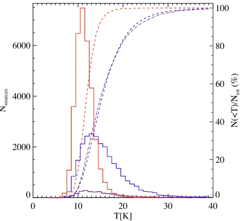
6.2 Dust temperature

The distributions of grey-body temperatures of the sources are shown in Fig.5. As already found by Giannini et al. (2012), Elia et al. (2013), Giannetti et al. (2013) and Veneziani et al. (2017) through Hi-GAL observations, but also by Olmi et al. (2009) through BLAST observations, the distributions of pre-stellar and protostellar sources show some relevant differences, the latter be-ing found towards warmer temperatures with respect to the for-mer. A quantitative argument is represented by the average values

¯

Tpre=12.0 K and ¯Tprt=16.0 K for pre-stellar and protostellar

sources, and the median values ˜Tpre=11.7 K and ˜Tprt=15.1 K,

respectively.

Furthermore, both the temperature distributions seem quite asym-metric, with a prominent high-temperature tail. This can be seen by means of the skewness indicator (defined asγ=µ3/σ3, whereµ3

is the third central moment and _σ is the standard deviation) of the two distributions:γpre=1.06 andγprt=1.40, respectively. The

positive skew, in this case, indicates that the right-hand tail is longer (γ =0 for a normal distribution), and quantifies that. On the other hand, the pre-stellar distribution appears more peaked than the pro-tostellar one. The kurtosis of a distribution, defined asδ=µ4/σ4

(whereµ4is the fourth central moment), is useful to quantify the

level of peakedness (for a normal distribution,δ=3). In these two cases, the kurtosis values are found to be quite different for the two distributions (_δpre=3.67 andδprt=3.04, respectively). Finally, we

also plot the cumulative distributions of the temperatures, which is another way to highlight the behaviours examined so far. We find

Figure 5. Grey-body temperature distributions for the pre-stellar (red his-togram) and protostellar (blue hishis-togram) sources considered for science analysis in this paper. Cumulative curves of the same distributions are also plotted as dashed lines (and the same colours), according to they-axis on the right-hand side of the plot. Finally, the temperature distribution of the sub-sample of MIR-dark protostellar sources is plotted in dark purple, and the corresponding cumulative as a dot–dashed dark-purple line.

that 99 per cent of the pre-stellar (protostellar) sources have dust temperatures lower than 18.1 K (33.1 K), and the temperature range widths required to go from 1 per cent to 99 per cent levels are 9.9 and 24.2 K, respectively.

These findings can be regarded from the evolutionary point of view: While pre-stellar sources represent the very early stage (or ‘zero’ stage) of star formation and, as such, are characterized by very similar temperatures, protostellar sources are increasingly warmer as the star formation progresses in their interior (e.g. Battersby et al.

2010; Svoboda et al.2016), so that the spanned temperature range is larger and skewed towards higher values. A prominent high-temperature tail should be regarded, in this sense, as a signature of a more evolved stage of star formation activity.

To corroborate this view, we consider the temperatures of the sub-sample of protostellar sources of our catalogue lacking a de-tection in the MIR (i.e. at 21 and/or 22 and/or 24µm, hereafter MIR-dark sources, as opposed to MIR-bright), whose distribution is also shown in Fig.5. They represent 10 per cent of the total protostellar sources (therefore dominated by MIR-bright cases). The average and median temperature for this class of objects are

¯

TMd=16.0 K and ˜TMd=14.8 K, respectively, i.e. halfway between

the values found for pre-stellar sources and those for the whole sample of protostellar ones, which is dominated by MIR-bright sources.

The reader should be aware that the dust temperature discussed here is derived simply from the grey-body fit of the SED at λ≥160µm and represents an estimate of the average tempera-ture of the cold dust in the clump. Using line tracers, it is possible to probe the kinetic temperature of warmer environments, such as the inner part of protostellar clumps, which is typically warmer (T_>

20 K, e.g. Molinari et al.2016b; Svoboda et al.2016) than the me-dian temperature found here for this class of sources. Despite this, as seen in this section, the grey-body temperature can help to infer the source evolutionary stage, and turns out to be particularly effi-cient in combination with other parameters, as further discussed in Section 7.

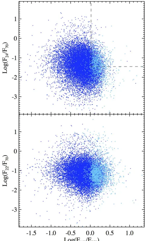
6.2.1 Herschelcolours and temperature

The availability of dust temperatures derived from grey-body fits makes it possible to directly compare withHerschelcolours (cf. Elia et al.2010; Spezzi et al.2013), to ascertain which ones are better representative of the temperature. In Fig.6, the source temperature is plotted versus the 10 possible colour pairs that can be obtained by combining the fiveHerschelbands (for each combination, only sources detected at both wavelengths are displayed). We designate as colour the decimal logarithm of the ratio of fluxes at two different wavelengths. Since the 70-µm band is not involved in the temper-ature determination, the colours built from it [plots (a)–(d)] do not show any tight correlation with temperature, while for the remain-ing six colours such correlation appears more evident, especially for those colours involving the 160-µm band. The best combination of spread of colour values (which decreases the level of temperature degeneracy, mostly at low temperatures) and agreement with the analytic behaviour expected for a grey body is found for colours involving the flux at 160µm [panels (e)–(g)]. In particular, for the

F500/F160colour, the grey-body curve has the shallowest slope, so

that we propose this colour as the most suitable diagnostic of the average temperature in the absence of a complete grey-body fit. For the case of SPIRE-only sources, lacking a counterpart at 160

µm, only three colours are available, but their relation with dust temperature [cf. panels (h)–(j)] appears to be affected by a high degree of degeneracy, making these colours unreliable temperature indicators.

Figure 6. Panels (a)–(j): plots of source temperature (as derived through the grey-body fit) versus all colours obtainable from possible pair combinations of the five Hi-GAL wavebands. Each plot is obtained using all sources provided with fluxes at the two involved wavelengths, specified at the bottom of the panel. The unnatural vertical cut of the point distribution in panel (j) is an artefact due to one of the filters adopted for source selection, ruling out sources withF350<F500(rescaled fluxed are considered, see Section 3.1).

The grey-dashed line represents the temperature of a grey body withβ=2.

6.3 Mass and surface density

Once source masses are obtained, it would be straightforward to show and analyse the resulting distribution (clump mass func-tion, hereafter ClumpMF). However, since such discussion implies considerations about the clump mass–size relation and, somehow equivalently, the surface density, we postpone the analysis of the ClumpMF until the end of this section, after having dealt with those preparatory aspects.

A meaningful combination of source properties is represented by the massMversus radiusrdiagram, which has been shown to be a powerful tool for investigating the gravitational stability ofHerschel

Properties of Hi-GAL clumps in the inner Galaxy

111

Figure 7. Top left-hand panel: mass versus radius plot for starless sources. Pre-stellar (red) and starless (green) sources are separated by the lineM(r)= 460 M(r/pc)1.9_{(Larson1981) (dot–dashed black line) (see Section 3.5). The areas of the mass–radius plane corresponding to combinations fulfilling the}

Kauffmann & Pillai (2010) and Krumholz & McKee (2008) thresholds for compatibility with high-mass star formation are filled with light blue and purple, respectively, the latter being contained in the former, and both delimited by a darker dotted line. Notice that adopting a lower limit of 10 Mfor the definition of a massive star, and a star formation efficiency factor of 1/3 for the core-to-star mass transfer as in Elia et al. (2013), these zones cannot extend below 30 M. Top right-hand panel: the same as in top left-hand panel, but for protostellar sources. Bottom left-hand panel: source density isocontours representing the pre-stellar and protostellar distributions displayed in the two upper panels of this figure. Densities have been computed by subdividing the area of the plot in a grid of 70×70 cells; once the global maxima for both distributions have been found, the plotted contours represent the 2 per cent, 20 per cent and 70 per cent of the largest of those two peak values, so that the considered levels correspond to the same values for both distributions, to be directly comparable. The black solid line crossing the bottom part of the light-blue area represents the threshold of Baldeschi et al. (2017). Bottom right-hand panel: surface density distributions (solid histograms) for pre-stellar (red) and protostellar (blue) sources. Because surface density is a distance-independent quantity, all sources (with and without distance estimates) are taken into account to build these distributions. The cumulative curves are plotted with dashed lines, normalized to they-axis scale on the right-hand side. The zone corresponding to densities surpassing the Krumholz & McKee (2008) threshold is filled with purple colour.

shows the mass versus radius distribution for the sources analysed in this study. In the top left-hand panel, the starless sources are shown, while, to avoid confusion, the protostellar ones are reported in the top right-hand panel: Larson’s relation mentioned in Section 3.5 is plotted to separate the starless bound (pre-stellar) and unbound sources.

From this plot, it is possible to determine if a given source satis-fies the condition for massive star formation to occur, where such condition is expressed as surface density,, threshold. Krumholz & McKee (2008) established a critical value ofcrit=1 g cm−2

based on theoretical arguments. However, L´opez-Sepulcre, Ce-saroni & Walmsley (2010) and Butler & Tan (2012), based on observational evidence, suggest the less severe values of crit

= 0.3 and 0.2 g cm−2_{, respectively. Also, Kauffmann & Pillai}

(2010), based on empirical arguments, propose the thresholdM(r) >870 M(r/pc)1.33_{as a minimum condition for massive star}

for-mation. Finally, the recent analysis by Baldeschi et al. (2017) of the distance bias affecting the source classification according to the two aforementioned thresholds produced the further criterion

M(r) > 1282 M(r/pc)1.42_{. In the upper side, we represent the}

most (Krumholz & McKee2008) and the least (Kauffmann & Pil-lai2010) demanding thresholds, respectively, to allow comparison with the behaviour of our catalogue sources.

As reported in Table2, a remarkable fraction of sources appear to be compatible with massive star formation based on the three thresholds (defined asKM,BandKP, respectively), especially

Table 2. Hi-GAL sources with the mass–radius relation compatible with massive star formation according to the surface density thresholdsKP,B

andKM(see text).

> KP > B > KM

Counts Per cent Counts Per cent Counts Per cent Protostellar 11 210 71.3 10 012 63.7 2062 13.1 Pre-stellar 12 431 64.8 9973 52.0 546 2.8

source densities for both the pre-stellar and the protostellar source populations. The peak of the protostellar source concentration lies well inside the area delineated by the Kauffmann & Pillai (2010) relation, while the pre-stellar distribution peaks at smaller densities. Rigorously speaking, however, such considerations on the initial conditions for star formation should be applied only to the pre-stellar clumps, since in the protostellar ones part of the initial clump mass has already been transferred on to the forming star(s) or dissipated under the action of stellar radiation pressure or through jet ejection. In any case, the presence of a significant number of very dense pre-stellar sources translates into an interestingly large sample of targets for subsequent study of the initial conditions for massive star formation throughout the Galactic plane (see Section 8.1). For such sources, due to contamination between the two classes described in Section 3.5, a further and deeper analysis is requested to ascertain their real starless status, independently of the lack of aHerschel

detection at 70µm.

Notice that the fractions corresponding to the threshold of Kauffmann & Pillai (2010) reported in Table2appear remarkably lower than the quantity estimated by Wienen et al. (2015) for the ATLASGAL catalogue, i.e. 92 per cent. This discrepancy cannot be explained simply by the better sensitivity of Hi-GAL: Taking the sensitivity curve in the mass versus radius of Wienen et al. (2015, their fig. 23), we find that the majority of our sources lie above that curve. The main reason, instead, resides in the analytic form itself of the adopted threshold. As mentioned above, Baldeschi et al. (2017) show that, even in the presence of dilution effects due to distance, sources in the mass versus radius plot are found to follow a slope steeper than the exponent 1.33, so that large physical radii, typically associated with sources observed at very far distances, correspond to masses larger than the Kauffmann & Pillai (2010) power law. This is not particularly evident in our Fig.7since the largest probed radii are around 1 pc, and the large spread of temperatures makes the plot quite scattered. Instead, fig. 23 of Wienen et al. (2015) contains a narrower distribution of points (since masses were de-rived in correspondence to only two temperatures, both higher than 20 K), extending up tor6 pc: Atr1 pc, almost the totality of sources satisfy the Kauffmann & Pillai (2010) relation. Clearly, another contribution to this discrepancy can be given by the scatter produced by possible inaccurate assignment of the far kinematic distance solution in cases of unsolved ambiguity (see Section 3.4). The information contained in the mass–radius plot can be rear-ranged in a histogram of the surface density5

such as that in Fig.7, bottom right-hand panel. The pre-stellar source distribution presents a sharp artificial drop at small densities due to the removal of the unbound sources, which is operated alongM∝r1.9_{, i.e. at an almost}

5_{It is notable that if a grey body is fitted to an SED through equation (1),}

the surface density is proportional toτref(equation (3)), which is, in turn,

proportional toλ−0β(equation 2), withβ=2 in this paper. This implies that

a description based on the surface analysis is, for such sources, equivalent to that based on theλ0parameter.

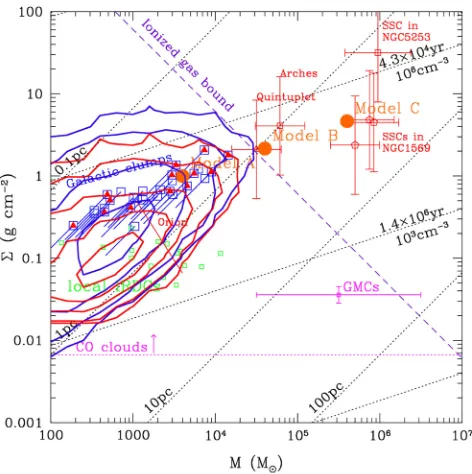
Figure 8. Plot of surface density versus mass of Tan (2005, his fig. 1), with overplotted number density contours of pre-stellar (red) and protostellar (blue) sources of our catalogue. The source density is computed in bins of 0.2 in decimal logarithm, and contour levels are 5, 20, 100, 250 and 500 sources per bin. The horizontal cut at lowest densities for red contours is due to the removal of starless unbound sources. The diagonal dotted lines represent the loci of given radii and number densities (and corresponding free-fall times). Typical ranges for molecular clouds are indicated with magenta lines, while the condition for the ionized gas to remain bound is indicated by the blue dashed line. Finally, locations for a selection of IRDCs (green squares), dense star-forming clumps (blue squares), massive clusters (red symbols) and cluster models of Tan (2005) (filled orange circles) are shown. Additional information reported in this diagram is provided in Tan (2005) and Molinari et al. (2014, their fig. 11).

constant surface density (M∝r2_{). Instead, despite the considered}

pre-stellar population being globally more numerous than the pro-tostellar one, at high densities ( 1 g cm−2_{) the latter prevails}

over the former. The protostellar distribution, in general, appears shifted towards larger densities, compared with the pre-stellar one, as can be seen in the different behaviour of the cumulative curves, also shown in the figure. This evidence is in agreement with the result of He et al. (2015), based on the MALT90 survey. Further evolutionary implications will be discussed in Section 7.3.

We note, as discussed in Section 6.1, that the compact sources we consider may correspond, depending on their heliocentric distance, to large and in-homogeneous clumps with a complex underlying morphology not resolved withHerschel. On one hand, this implies that the global properties we assign to each source do not remain necessarily constant throughout its internal structure; thus, a source fulfilling a given threshold on the surface density might, in fact, contain sub-critical regions. On the other hand, in a source with a global sub-critical density, super-critical portions might actually be present, leading to misclassifications; for this reason, the numbers reported in Table2should be taken as lower limits.

Properties of Hi-GAL clumps in the inner Galaxy

113

Figure 9. Clump mass function for pre-stellar (red filled histogram) and protostellar (blue histogram) sources, obtained in 0.5-kpc-wide heliocentric distance ranges. Each panel corresponds to the range that is reported in the upper part. The dashed red and blue lines indicate the completeness limits, and the solid red and blue vertical lines indicate the lower limit used to fit the curves in Fig.10, for the pre-stellar and protostellar cases, respectively.

values from the final Hi-GAL physical catalogue. The Hi-GAL sources are found to lie in the regions quoted by Tan (2005) for Galactic clumps and local IRDCs. In the upper right-hand part of their distribution, they graze the line representing the condition for ionized gas to remain bound. This plot summarizes the nature of the sources in our catalogue: clumps spanning a wide range of mass/surface density combinations, with many of them found to be compatible with the formation of massive Galactic clusters.

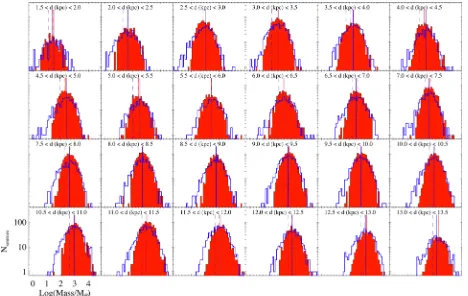
6.4 The ClumpMF

The ClumpMF is an observable that has been extensively stud-ied for understanding the connection between star formation and parental cloud conditions. Although formulations are quite similar, the ClumpMF should not be confused with the core mass func-tion (hereafter CoreMF), typically studied in nearby star-forming regions (d 1 kpc). Differences between these two distributions will be discussed later in this section.

Large IR/sub-mm surveys generated numerous estimates of the ClumpMF (e.g. Reid & Wilson2005,2006; Eden et al.2012; Tack-enberg et al.2012; Urquhart et al.2014a; Moore et al.2015). Like-wise, data from Hi-GAL have been used for building the ClumpMF in selected regions of the Galactic plane (Elia et al.2013; Olmi et al.

2013).

Building the mass function of a given sample of sources (Hi-GAL clumps in the present case) requires a sample to be defined in a consistent way. A clump mass function built from a sample of sources spanning a wide range of distances (as in our case) would

be meaningless, since at large distances low-mass objects might not be detected or might be confused within larger, unresolved struc-tures (see Appendix C); therefore, it makes little sense to discuss it. Therefore, we first subdivide our source sample into bins of helio-centric distance, and then build the corresponding mass functions separately. In addition, as pointed out, e.g. by Elia et al. (2013), it is more appropriate to build separate ClumpMFs for pre-stellar and protostellar sources. Strictly speaking, only the mass distribu-tions of pre-stellar sources are intrinsically coherent, as the mass of the protostellar sources does not represent the initial core mass, but rather a lower limit, which depends on the current evolutionary stage of each source.

In Fig.9, the clump mass functions are shown. They have been calculated using sources provided with a distance estimate, from 1.5 to 13.5 kpc in distance bins of 0.5 kpc, in logarithmic mass bins, and separately for pre-stellar and protostellar clumps.

It can be immediately noticed that, for any distance range, the protostellar ClumpMF is wider than the pre-stellar one, so that a deficit of pre-stellar clumps with respect to protostellar ones is seen both at lowest and highest masses in each bin of distance. The former effect is mostly due to sensitivity: Sure enough, thanks to higher temperature, a protostellar source can be detected more easily than a pre-stellar source of the same mass. For example, according to equation (C2) in Appendix C2, applied to a given mass, the flux of a source atT= 15 K (i.e. ∼T¯prt) is nearly twice that of

a source atT=12 K (i.e.∼T¯preK). The latter effect can in part