White Rose Research Online URL for this paper:
http://eprints.whiterose.ac.uk/116534/
Version: Accepted Version
Article:
Baldivieso Monasterios, P.R. and Trodden, P. orcid.org/0000-0002-8787-7432 (2017)
Low-Complexity Distributed Predictive Automatic Generation Control with Guaranteed
Properties. IEEE Transactions on Smart Grid. ISSN 1949-3053
https://doi.org/10.1109/TSG.2017.2705524
© 2017 IEEE. Personal use of this material is permitted. Permission from IEEE must be
obtained for all other users, including reprinting/ republishing this material for advertising or
promotional purposes, creating new collective works for resale or redistribution to servers
or lists, or reuse of any copyrighted components of this work in other works.
[email protected] https://eprints.whiterose.ac.uk/ Reuse
Unless indicated otherwise, fulltext items are protected by copyright with all rights reserved. The copyright exception in section 29 of the Copyright, Designs and Patents Act 1988 allows the making of a single copy solely for the purpose of non-commercial research or private study within the limits of fair dealing. The publisher or other rights-holder may allow further reproduction and re-use of this version - refer to the White Rose Research Online record for this item. Where records identify the publisher as the copyright holder, users can verify any specific terms of use on the publisher’s website.
Takedown
If you consider content in White Rose Research Online to be in breach of UK law, please notify us by
Low-Complexity Distributed Predictive Automatic
Generation Control with Guaranteed Properties
Pablo R. Baldivieso Monasterios and Paul Trodden,
Member, IEEE
Abstract—An automatic generation control scheme for multi-area power systems is presented, based on the technique of distributed model predictive control. Local area controllers solve nested MPC problems in order to regulate states to steady values, and reject the disturbances induced by tie-line interactions. The approach achieves guaranteed constraint satisfaction, recursive feasibility of the MPC problems and stability, while maintaining on-line complexity similar to conventional MPC. A rigorous off-line design methodology is given for selecting controller parameters, and is demonstrated on an example 4-area system.
Index Terms—Load frequency control; automatic generation control; model predictive control; distributed control.
I. INTRODUCTION
M
ODERN electrical power networks typically comprise a number ofcontrol areas, each managed and operated separately by regional-, independent- or transmission-system operators (RTOs, ISOs or TSOs), and interconnected via alternating current (AC) or high-voltage direct current (HVDC) lines. Within these networks, load-frequency control (LFC) is a fundamental responsibility of each area operator, and is the problem of providing the necessary control actions within the area in order to meet local demand, maintain reserve levels for primary frequency controllers, and assist in keeping system frequency and tie-line flows close to nominal values.The problem of desiging automatic generation control (AGC) schemes to fulfil the LFC function has attracted attention since the 1950s. Numerous approaches have been proposed, utilizing a broad range of classical and modern control techniques (see, for example, [1]–[3] for recent surveys on the topic). The AGC resides at the secondary level of the traditional frequency control hierarchy, one layer above the primary (droop) control, and the objectives and requirements upon it are well understood [4]. In the simplest case of a single area controlled by a single operator, the LFC function can be achieved by adding an integral control loop to the conventional droop (proportional) control in order to eliminate offset in frequency. Multiple area LFC is, on the other hand, a more challenging problem owing to the non-centralized but interconnected organization of the network—each area being operated independently, but with scheduled power flows between areas—and uncoordinated decision making can lead to errors, constraint and contract violations and even instability. Model predictive control (MPC) has long been identified as a leading candidate technique for LFC/AGC, and, more generally, control problems in future power networks and smart grids.
P. R. Baldivieso and P. A. Trodden are with the Department of Automatic Control & Systems Engineering, University of Sheffield, Mappin Street, Sheffield S1 3JD, UK (e-mail: {prbaldivieso1, p.trodden}@shef.ac.uk).
MPC is a well established, advanced control technique, popular in industry [5] (particularly in process control [6]), and with mature theoretical foundations [7], [8]. It excels in situations where a control law is prohibitively difficult to determine offline, such as in the presence of constraints. Because the control law is implicitly (rather than explicitly) defined by the repeated solving of an optimal control problem on-line, MPC is able to handle constraints naturally and systematically. Moreover, because an objective function is optimized every time the optimal control problem is solved, MPC is advantageous for systems where an economic cost is to be minimized, or a performance metric is to be maximized.
the approach is fully decentralized and—moreover—relies on restricting constraints in a conservative manner, leading to potentially poor performance [17]. Secondly, the scheme requires the explicit characterization, computation and use of
robust control invariant sets [18], the complexity of which grows prohibitively with system order; thus, each area’s dynamics are practically limited to second or third order.
The aim of this paper is to develop a DMPC-based AGC scheme that is implementable (in terms of the complexity of the on-line computations and the ease of design) yet achieves the desirable properties of guaranteed constraint satisfaction, feasibility and stability. To this end, we propose a scheme that— similar to [16] and other DMPC approaches with guaranteed properties [19]–[21]—utilizes the “tube” concept from robust MPC [22], but with key differences, the enumeration of which also serves to define the contribution of the paper:
1) We present a distributed MPC-based approach to the multi-area AGC problem that attains the desirable guar-antees closed-loop stability, recursive feasibility and constraint satisfaction without the need for supervision or iteration/negotiation between controllers.
2) The distributed AGC employs a “nested” approach to DMPC, based on the tube approach to robust MPC [22], wherein the overall control law comprises two parts. The first part arises implicitly from the solution of a conventional MPC problem (albeit with tightened constraints), and steers the local system states to steady-state values. The second part rejects the effects of disturbances acting on the local system; here, the mutual interactions arising from the physical coupling of areas. This second control law is—uniquely among DMPC approaches—defined by a secondary MPC problem, which is able to take into account shared information from other area controllers, plus a robust control law based on disturbance-invariant sets.
3) A distributed, offline design methodology is presented for the rigorous determination of controller parameters. In particular, we exploit the theory of disturbance-invariant sets in order to compute, via the solving of a two linear programs (LPs) for each area, the scaling factors to apply to constraints in the MPC problems in order that their satisfaction is guaranteed, and the robust control law. The invariant sets—which can be very complex objects for systems of third- or higher-order—are, however, merely implicit, and are never explicitly constructed or included in the MPC problems; thus, the complexity of the MPC problems is similar to conventional MPC. This permits the application of the proposed approach to systems with higher-order local dynamics, such as the fourth-order power systems studied in this paper.
A companion paper to this one, [23], presents the nested DMPC approach in detail, including theoretical results and proofs. In this paper, we present the core details of the approach while limiting theoretical details and keeping the paper self contained. The next section defines the LFC problem. In Section III, the proposed AGC is presented, including MPC optimization problems and control algorithm. The controller design
proce-dure and theoretical properties are given in Section IV. The proposed approach is applied to an example 4-area system in Section V. Finally, concluding remarks are made in Section VI.
II. THELOADFREQUENCYCONTROLPROBLEM
A. Multi-area Power System Model
We consider a network of M areas, where, in normal operation, the frequency dynamics of area i ∈ {1, . . . , M}
are governed by the classical linearized swing equation
Mi∆ ˙ωi= ∆pmi −∆p
e
i, (1)
where ∆ωi is the deviation of the aggregate rotor speed, normalized to nominal/rated value (p.u.). The parameter,Mi, is the aggregate mechanical starting time (seconds; equal to twice the inertia constant Hi). The right-hand side variables ∆pm
i and ∆pei represent, respectively, the deviation of the mechanical (input) power from nominal (p.u.) and the deviation of the electrical (output) power from nominal (p.u.). The latter comprises the load power deviation (from its nominal value) in areai—consisting of a frequency independent component, ∆pd
i, and a frequency dependent componentDi∆ωi—and the net tie-line power deviation between areaiand connected areas
j∈ Ni:
∆pei= ∆pdi+Di∆ωi+
X
j∈Ni
∆pij. (2)
The tie-line power deviation∆pijis modelled by the linearized power flow equation
∆ ˙ptiei = X j∈Ni
∆ ˙pij =
X
j∈Ni
Pijs(∆ωi−∆ωj) (3)
where Ps
ij is the synchronizing power coefficient of line(i, j) and is assumed constant.
Combining (1)–(3) leads to the conventional damped swing model1
Mi∆ ˙ωi+Di∆ωi= ∆pmi −∆p
d
i −∆p
tie
i . (4)
In area i, the aggregated turbine and governor dynamics are modelled by the following simplified dynamics. A speed governor provides an output power in response to the difference between the reference, or setpoint, power,∆pref
i , and the droop power R1∆ωi, whereRis the regulation factor, and is assumed to have first-order dynamics with time constantTig:
Tig∆ ˙pvi =−∆pvi+ ∆prefi − 1
R∆ωi (5)
The turbine (prime mover) provides the mechanical power ∆pm
i—the input to the power system in areai—in response to ∆pv
i, and is assumed to have time constantTit:
Tit∆ ˙pmi =−∆pmi + ∆pvi. (6)
Note that more detailed models of the system can be considered, provided that the underlying dynamic models are linear; however, we consider this simplified, fourth-order model to simplify the exposition of the proposed distributed control.
1Here, the “damping power”D
i∆ωiarises from the frequency-dependent
B. AGC Objective and Constraints
The objective of the AGC is to provide secondary-level control in order to maintain—despite changes to load—the system frequency close to nominal, tie-line power interchanges close to scheduled values, and a sufficient level of reserve for the primary frequency (droop) control. Typically, the Area Control Error (ACE),
ACEi=βi∆ωi+
X
j∈Ni ∆pij
is the performance measure of success of the AGC with respect to meeting this goal, and should be maintained in each area close to—and preferably at—zero. Note that, if∆ωiis regulated to zero in each area, despite load changes∆pd
i, then ACEi= 0 and the goal is achieved. In fact, note that
(∆ptie
i ,∆ωi,∆pmi,∆piv) = (0,0,∆pdi,∆pdi)
is an equilibrium for the system, when the load deviation in area iis∆pd
i, under the steady-state control∆prefi = ∆pdi. During operation of the network, any constraints should be satisfied. Constraints may arise from physical or operational limits, or from considerations of safety or economy. In this paper, we allow for all system variables be constrained in a general way; in particular, defining the state of area ias xi= (∆ptie
i ,∆ωi,∆pmi,∆p
v
i) and its control input as ui = ∆prefi , we express the constraints as
xi∈Xi ui∈Ui (7)
This includes, for example, the case of simple bounds on some or all of the variables (e.g,|∆ωi| ≤Ω). Assumptions on the sets Xi andUi will be given in Section III-C.
The problem we consider is design of a distributed AGC scheme for the multi-area system, in order to maintain ACE around zero, despite load disturbances, while satisfying all constraints. By distributed, we mean that the control of the multi-area system is performed by a set of independent controllers that may exchange information: each control area is managed by a single controller that provides the signalui in response to both local area information and information shared between areas.
Remark 1: From the perspective of each area, which may itself be a large and interconnected power system, the control is centralized and the control signal ui (the reference power) needs to be allocated to individual producers and generating units. The standard approach is to use participation factors, as explained in [24] and employed in, for example, [14] in the deregulated power system context. We consider this aspect of the AGC problem to be beyond the scope of this paper, which is focused on developing—at the whole-system scale—a multi-area control strategy with theoretical guarantees.
Remark 2:The fourth-order system (1)–(6) is an aggregated, reduced-order model of the true dynamics within each area. As such, it contains internal, “fictitious” states—aggregated governor and turbine power deviations—that have no direct physical meaning and cannot be measured in a real system. However, their presence means that the model captures more accurately the dynamics of power and frequency within each
area. In Section III, the control algorithm we propose assumes, for simplicity, full state measurements, including of these internal states; however, we discuss how these states can be estimated from available measurements in a real power system.
C. The Challenge for Control
The continuous-time dynamics of areai may be written in the compact form
˙
xi= ¯Aiixi+ ¯Biui+ ¯Biddi+
X
j∈Ni ¯
Aijxj. (8)
This model is linear with two disturbances: the first disturbance,
di, is the load power deviation∆pdi. The second disturbance arises from the dynamic coupling (the dependence ofx˙i on
xj), itself a consequence of the physical connection (tie-lines) between areaiand areasj∈ Ni.
A compound, centralized model of the multi-area system may be obtained as
˙
x= ¯Ax+ ¯Bu+ ¯Bdd (9)
where x, u and d are the stacked vectors of all the xi,
ui and di respectively. The second disturbance—from the dynamic coupling between areas—disappears, being absorbed into the term Ax, and leading to a conventional linear model with process disturbance. For this problem—of rejecting the disturbance dwhile satisfying all constraints—the ingredients sufficient to synthesize an MPC controller with guarantees are well known [7]; however, the control law u = κ(x) is centralized and permits the dependence of the controlui for areaion states xj for areas j6=i.
The non-centralized problem—of designing area-by-area control laws that achieve the control objective collectively—is more challenging, for at least two reasons. Firstly, the control problems are coupled via the states, and cannot be solved independently. To circumvent this, a decentralized (ignoring coupling) or distributed (with information shared between areas) approach may be taken. In either case, constraint satisfaction and stability are not easy to guarantee, since the actions of the controller are based on missing or inaccurate state information. The second reason is specific to MPC, because a discrete-time model of the system dynamics is usually required. (Continuous-time formulations are emerging, but are subject to computational and practical hurdles [25], [26]). Exact discretization of the centralized dynamics destroys sparsity in the system matrices( ¯A,B¯); decomposing the discrete-time centralized system leads to M discrete-time local systems densely coupled via statesandinputs. In other words, artificial (rather than physical) direct links are created between areas in order to retain accuracy of the discrete-time model (c.f., Kron reduction). Inexact discretization methods, on the other hand, can maintain sparsity but the accuracy of the prediction model is compromised; closed-loop performance can suffer.
III. DISTRIBUTEDPREDICTIVEAGC
In this section, the proposed distributed predictive AGC is presented, beginning with a description of the control architecture and laws, and concluding with formal definitions of the MPC optimization problems and the control algorithm.
A. Control Architecture for Area i
We discretize the dynamics of the system on an area-by-area basis; that is, discretization of each of the local area models (8), rather than discretization of the composite model (9). The zero-order hold discretization method is employed because of its accuracy and suitability to MPC: it models well how the MPC controller provides controls to the real plant, as piecewise constant signals, and, in fact, is usually an exact method. Inexactness arises in this case because of how the interactions are modelled, as exogeneous disturbances acting on each area. However, this approach preserves the sparsity in the system-wide dynamics2, and has the advantage that the discretization process requires only local knowledge about areai plus theAij, which depends on only the synchronizing power coefficient of tie-line (i, j). The resulting discrete-time counterpart to (8) is
x+i =Aiixi+Biui+Biddi+
X
j∈Ni
Aijxj (10)
where x+i is the successor state.This model still cannot be employed directly within an MPC optimization problem for area i, owing to the state coupling—the dependency onxj. To decouple area models, we express the net action of the state coupling as a local disturbance acting on the dynamics of i:
x+i =Aiixi+Biui+Biddi+wi,
where wi ,Pj∈NiAijxj. We then define a nominalmodel of the local area dynamics
¯
x+i =Aiix¯i+Biu¯i+Biddi. (11)
This model, which omits the state coupling and depends on only local variables, can then be used for predictions within a conventional MPC controller; this would define an implicit nominal control lawu¯0
i−ussi = ¯κi(¯xi−xssi). The direct use of
ui= ¯u0i as the control action is problematic, however, because the interactions (disturbanceswi) have been entirely neglected; the controller is non-robust and constraint satisfaction is not
guaranteed for anything other than wi≡0.
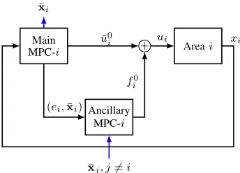
We take, therefore, a robust approach to this problem by employing a second, ancillary, controller in order to reject the disturbances; see Figure 1. The ancillary controller acts on the
error between true statexi and nominal statex¯i, defined as
ei ,xi−x¯i. This error is governed by the dynamics
e+i =Aiiei+Bifi+wi, (12)
where fi ,ui−u¯i. The main idea, then, is for the overall control system to employ a two-degree-of-freedom control law
ui−ussi = ¯κi(¯xi−xssi) +κi(ei),
2For an interesting discussion of, and contribution to, sparsity-preserving
discretization, see [27]
Areai
Main MPC-i
Ancillary MPC-i
+ ¯
u0 i
¯
xi
f0 i
ui xi
(ei,x¯i)
¯
[image:5.612.349.521.56.180.2]xj, j6=i
Fig. 1. Block diagram of the proposed DMPC-AGC. The main MPC computes the optimal nominal control u¯0
i based on local state measurements. The
ancillary MPC provides a controlf0
i, computed taking into account shared
predictionsx¯jfrom other control areas.
which is intended to steer the nominal system (¯xi,u¯i)to its steady state and, in turn, regulate the error system(ei, fi)to zero. For the latter, we propose an ancillary MPC controller, which uses information about the planned trajectories from the connected areas, and is described next.
B. Ancillary Controller Description
The aim of the ancillary controller is to drive the error ei to zero, while satisfying constraints. This error is governed, however, by the uncertain dynamics (12); a robust controller could be designed, but the problem here is that disturbancewi is not just a random signal to be rejected, but is a well-behaved input directly related to the state trajectories of other areas, about which information can be obtained.
Therefore, the approach we take is to split the error,ei, into a planned part, ¯ei, and an unplanned part,eˆi. The former is regulated by a secondary MPC controller, which is able to take into account the shared predictions from other areas, while the latter is regulated by a robust controller. In order to design the ancillary MPC, we define asecond nominal model for area i
ˆ
x+i =Aiixˆi+Biuˆi+Biddi+
X
j∈Ni
Aijx¯j. (13)
This model includesplannedstates, ¯xj, for other areas instead of true states,xj. Defining ¯ei,xˆi−x¯i, we obtain
¯
e+i =Aiie¯i+Bif¯i+ ¯wi (14)
where f¯i ,uˆi−u¯i and w¯i ,Pj∈NiAijx¯j, and make the following observations: this model of the error involves only nominal states and inputs, plus aplanned disturbancew¯i that arises from the planned trajectories of other control areas; therefore, this planned error model is suitable for use as a prediction model within an MPC controller, to steere¯i to zero. At this point, we note, however, that the planned error is not the same as the true error. In particular, if ei=xi−¯xi and ¯
ei= ˆxi−x¯i, then
(ei−¯ei)+=Aii(ei−¯ei) +Bi(fi−f¯i) +
X
j∈Ni
Aijej.
We define this residual error as theunplanned erroreˆi=ei−¯ei, alongside an unplanned disturbancewˆi,Pj∈NiAijej, so
ˆ
Therefore, as proposed, the error ei = ¯ei + ˆei has been split into a planned part and an unplanned part; note that
wi= ¯wi+ ˆwi. We propose to handle the planned part via an ancillary MPC control law f¯i0= ˆκi(¯ei; ¯wi)—wherew¯i is the sequence of planned disturbances obtained from the predictions of other areas—and the unplanned part via a robust control law
ˆ
fi= ˜κi(ˆei). Thus, the control law of the ancillary controller is
fi0=κi(ei) = ˆκi(¯ei; ¯wi) + ˜κi(ˆei) = ¯fi0+ ˆfi. (16)
The overall control law for area iis then
ui = ¯u0i+f
0
i =u
ss
i + ¯κi(¯xi−xssi) + ˆκi(¯ei; ¯wi) + ˜κi(ˆei). (17) This law has the advantage, among others, that is conceptually clear in the sense that each term of the law is aimed to tackle a different problem. The first term regulates the nominal subsystem to its steady state values; the second term drives the planned error to zero using the information arising from the neighbouring areas; the third term provides robustness to unplanned errors and disturbances. The precise definitions and detailed synthesis of these terms in the control law are presented in later in this section. Before that, we describe how the planned and unplanned disturbances may be bounded, which is a prerequisite to taking a robust control approach.
C. Bounding Local Area Disturbances
The state and input for areaiare subject to the constraints (7), about which we make the following assumption.
Assumption 1: The set Xi is a polyhedral, the set Ui is polytopic, and each contains the origin in its interior.
To explain our terminology, we define a polyhedron as the (convex) intersection of a finite number of closed halfspaces, and a polytope as a bounded polyhedron. Therefore, the state constraint set may be unbounded, but the input constraint set is required to be bounded.
If xj ∈Xj, it follows thatwi =Pj∈NiAijxj is bounded within a setWi, given by
Wi, M
j∈Ni
AijXj (18)
In this definition, the symbol L
denotes the Minkowski summation of the setsAijXj, overj ∈ Ni, and whereAijXjis the linear mapping of the setXj by the matrixAij, defined as
{Aijxj :xj ∈Xj}. The Minkowski sum of two setsA ⊂Rn andB ⊂Rn isA ⊕ B,{a+b:a∈ A, b∈ B}.
Assumption 2:The disturbance setWi is a polytope satisfy-ing Wi⊂interior (Xi).
Essentially, Assumption 2 is a weak-coupling assumption that limits the strength of inter-area tie lines. Moreover, it is a necessary assumption in order for the controller design procedure described in Section IV-B to succeed. On the other hand, when the coupling is sufficiently weak it is an assumption that is easy to meet by judicious selection of the state constraints. In particular, owing to the structure of the multi-area dynamics, it is sufficient to impose state constraints on only the frequency deviation in each area in order to guarantee thatWi is polytopic (closed and bounded). This has the added advantage that there is no need to impose constraints
on the other, internal states, which would have no clear physical meaning.
We note that the disturbancewi=Pj∈NiAijxj is bounded provided that statesxj satisfy constraints. However, we have split xj into a nominal part plus error: xj = ¯xj+ej. Thus, our approach is to ensure, via the main MPC, thatx¯j∈αxjXj, where αx
j ∈[0,1), and, via the ancillary controller, thatej ∈ (1−αx
j)Xj. Then xj ∈ Xj and, moreover, w¯i and wˆi are bounded within polytopesW¯i andWˆi; these sets are defined later.
D. Main MPC-i Optimization Problem
Recall that the main MPC controller steers the states of areai to steady-state values, using the nominal (disturbance-free) prediction model (11). The associated MPC optimization problem is defined as follows.
¯
Vi
0
(¯xi;di) = min
¯
ui N−1
X
k=0
ℓi x¯i(k)−xiss,u¯i(k)−ussi
(19)
subject to, fork= 0. . . N−1,
¯
xi(0) = ¯xi, (20a) ¯
xi(k+ 1) =Aiix¯i(k) +Biu¯i(k) +Biddi, (20b) ¯
xi(k)∈αxiXi, (20c) ¯
ui(k)∈αiuUi, (20d) ¯
xi(N) =xssi. (20e)
The stage cost function is, for simplicity, quadratic:
ℓi(xi, ui),x⊤i Qixi+u⊤i Riui,
where Qi and Ri are positive-definite matrices. The input and state constraint sets are scaled by factors(αxi, αui); how these scaling factors are selected in order to ensure constraint satisfaction and recursive feasibility of the optimization problem will be described in Section IV. In regard to the load disturbance
di, and the availability of measurements to the controller, we make the following assumptions.
Assumption 3 (Piecewise constant disturbances):The distur-bancedi= ∆pdi for areaiis piecewise constant.
Assumption 4 (State and disturbance measurements):The statexi and disturbancedi are known at each time instant by the local controller.
Remark 3: In practice, of course, accurate measurements of the states and disturbances are not available, and estimates must be used. In that case, it is conventional in MPC to employ a state observer [28], which provides both state estimates and disturbances. In the distributed setting of MPC, our previous work [29]—based on [30]—shows how the robust control approach can be extended to handle only (noisy) output measurements, with only limited modifications and modest additional complexity, while maintaining theoretical guarantees. In the current paper, however, we make Assumption 4 in order to focus on the LFC control problem, rather than the whole estimation and control problem, and keep the presentation concise and simple.
requires an initial state measurement, or estimate, in order to provide predictions. In a real power system, not all of these states have direct physical meaning or can be measured. However, we note that the model is fully observable from measurements of either the tie-line power flows or local area frequency. Therefore, if tie-line flow or frequency measure-ments are available, then all states can be estimated.
Note that the state xi is not required by the main MPC controller, which propagates its own internal state x¯i, but rather the ancillary controller in order to determine the error
xi − x¯i. The disturbance measurement is used in order to calculate the steady-state equilibrium pair (xss
i, ussi); the following assumption applies to these values.
Assumption 5 (Steady state feasibility): For each areai, the steady-state values satisfy xss
i ∈αxiXi andussi ∈αuiUi. The solution of the main MPC problem is the control sequence u¯0
i ,
¯
u0
i(0),u¯0i(1), . . . ,u¯0i(N −1) , from which the following implicit control law is defined:
¯
u0i =ussi + ¯κi(¯xi−xssi) =u
ss
i + ¯u0i(0).
Next, we define the ancillary MPC-i optimization problem, yielding the remaining terms of the control law (17).
E. Ancillary MPC-i Optimization Problem
The prediction model (14) employed by the ancillary controller uses information (state predictions) obtained from connected areas. This information originates from the solutions of the main optimization problems, to form the sequence of planned disturbances w¯i=
¯
wi(0),w¯i(1), . . . ,w¯i(N) . With this, the ancillary MPC optimization problem is defined as
ˆ
Vi0(¯ei; ¯wi) = min¯
fi H−1
X
k=0
ℓi e¯i(k),f¯i(k)
(21)
subject to, fork= 0. . . H−1,
¯
ei(0) = ¯ei, (22a) ¯
ei(k+ 1) =Aiie¯i(k) +Bif¯i(k) + ¯wi(k), (22b) ¯
ei(k)∈βxiXi, (22c) ¯
fi(k)∈βuiUi, (22d) ¯
ei(H) = 0. (22e)
Similar to the main problem, the constraints are scaled by factorsβx
i andβui; the selection of these scaling constants will be described in the next section. The prediction horizon of this problem isH; since the disturbance sequence satisfiesw¯i(N) = 0, then settingH ≥N+ 1 will ensure that the disturbance is dealt with within the first N steps of the predictions, with the remaining H−N steps allowing drive the predicted error to zero, as required by the terminal constraint (22e).
Solving this problem yields the optimal control sequence
¯ f0
i ,{f¯i0(0),f¯i0(1), . . . ,f¯i0(H −1)} and, moreover, defines the implicit control law that is the first of the two terms in the ancillary control law (16):
¯
fi0= ˆκi(¯ei; ¯wi) = ¯fi0(0).
F. Ancillary Robust Control Law
The first term in the ancillary control law (16) handles the planned errore¯iin response to the planned disturbancew¯i. The unplanned erroreˆi, on the other hand, is perturbed (via (15)) by the unplanned disturbance, wˆi, which is non-deterministic. Therefore, for the second term in the ancillary control law we propose a robust controller based on the theory of robust invariant sets. To this end, we need the following definition.
Definition 1 (RCI set):A setRisrobust control invariant
(RCI) for a system x+ =f(x, u, w)and constraint set X,U and W if (i) R ⊂ X and (ii) for all x∈ R, there exists a
u∈Usuch thatx+=f(x, u, w)∈ R,∀w∈W.
In the context of the unplanned error dynamics (15), with the constraint sets defined (following the arguments in Section III-C) as (1−αx
i)Xi,(1−αui)Uiand the disturbance setWˆi that can now be defined as
ˆ
Wi , M
j∈Ni
(1−αxj)AijXj,
it is possible to define a RCI set, Rˆi, and an associated invariance-inducing control law˜κi(·)such that for any element of this set,eˆi∈Rˆi, the associated control action is
ˆ
fi= ˜κi(ˆei).
This robust control law is the second of the two terms in (16); its existence and design is discussed in Section IV.
G. Distributed Control Algorithm
Each area is controlled according to the following algorithm.
Algorithm 1 (Distributed Predictive AGC for Area i):
Initial data: Sets Xi, Ui; matrices(Aij, Bij) forj ∈ Ni; constantsαx
i,αui,βix,βiu; statesx¯i=xi(0),e¯i= 0,w¯i= 0, andVi∗= +∞.
Online Routine:
1) At timek, controller statex¯i and disturbancedi, solve (19) s.t. (20) to obtainu¯0
i and state predictionsx¯0i. 2) Transmitx¯0
i to controllersj∈ Ni. 3) Compute w¯0
i = {w¯0i(l)}l from received x¯0j, where ¯
w0i(l) =P
j∈NiAijx¯
0
j(l),l= 0. . . N.
4) At controller statee¯i, solve (21) s.t. (22) to obtain f¯i0: if feasible and Vˆi0(¯ei; ¯w0i) ≤ V
∗
i , set w¯i = ¯w0i and
Vi∗ = ˆVi0(¯ei; ¯wi0); else, solve (21) s.t. (22) using the previous disturbance sequence w¯i.
5) Measure local statexi, calculate ˆei=xi−x¯i−e¯i, and apply ui= ¯u0i + ¯fi0+ ˆfi, where fˆi= ˜κi(ˆei).
6) Update controller states asx¯+i =Aiix¯i+Biu¯0i +Biddi and e¯+i = Aiie¯i +Bif¯i0 + ¯wi, where w¯i = ¯wi(0), and w¯+
i = {w¯i(1), . . . ,w¯i(N),0} and V ∗+
i = V
∗ i −
ℓi(¯ei,f¯i0).
7) Setk=k+1,x¯i= ¯x+i ,¯ei= ¯e+i ,w¯i= ¯w+i ,V ∗ i =V
∗+
i , and go to Step 1.
second problem is guaranteed to be feasible, as established in Section IV-C. Next, we present in detail the design procedure for the scaling constants and robust control law.
IV. CONTROLLERDESIGN ANDTHEORETICALPROPERTIES
The design of the robust controller fˆi = ˜κi(ˆei), and subsequent selection of the scaling factors that restrict the constraints in the MPC problems, is based on the theory of optimized robust control invariance [18]; therefore, we begin with an introduction to the main concepts.
A. Optimized Robust Control Invariance
The optimized robust control invariance approach of [18] proposed a novel characterization of an RCI set for a system
x+=Ax+Bu+wand constraint set(X,U,W)as
Rh(Mh) = h−1 M
l=0
Dl(Mh)Wwithµ(Rh(Mh)) = h−1 M
l=0
MlW.
The setµ(Rh(Mh))is the set of invariance-inducing control actions, defined as µ(Rh), {µ(x) : x∈ Rh} = {u ∈U :
x+∈ Rh,∀w∈W}. The matrices Dl(Mh), l= 0. . . hare
D0(Mh) =I, Dl(Mh),Al+ l−1 X
j=0
Al−1−jBMj, l≥1
with Mj ∈ Rm×n and Mh , (M0, M1, . . . , Mh−1), such
that Dh(Mh) = 0; the latter is ensured by setting hgreater than or equal to the controllability index of (A, B). The set of matrices that satisfy these conditions is given by Mh ,
{Mh : Dh(Mh) = 0}. Constraint satisfaction is guaranteed
if Rh(Mh) ⊆ ηX and µ(Rh(Mh)) ⊆ θU, with (η, θ) ∈ [0,1]×[0,1].
As shown in [18], the linear programming (LP) problem to compute these sets is
min{δ:γ∈Γ}, (23)
where γ = (Mh, η, θ, δ), and the set Γ = {γ : Mh ∈
Mh,Rh(Mh) ⊆ ηX, µ(Rh(Mh)) ⊆ θU,(η, θ) ∈ [0,1]× [0,1], qηη +qθθ ≤ δ}; qη and qθ are weights to express a preference for the relative contraction of state and input constraint sets. Feasibility of this problem is linked to the existence of an RCI set: if (23) is feasible, then Rh(Mh) exists and satisfies the RCI properties [18].
B. Design Procedure
In our context, the RCI LP problem is useful because solving it provides an invariance-inducing robust control law—a suitable candidate for the third term in the overall control law— plus some scaling constants that outer-bound (with respect to the state and input constraint sets) the size of the RCI set and its corresponding set of control actions. Therefore, we employ the RCI LP problem as the key ingredient in the following design procedure, for each area. The design starts with determining an RCI set for the overall error,ei, and the overall disturbance set Wi, because the latter is known. The real aim is to determine an RCI control law for the unplanned error,eˆi, and unplanned
disturbance setWˆi; however, the latter is not known until the scaling constantsαx
i for each area have been determined. 1) The problem (23) associated with the dynamics e+i =
Aiiei+Bifi+wiand known constraint set(Xi,Ui,Wi) is solved to yieldγi,h= (Mi,h, ηi, θi, δi), whereηi and
θi are scalings ofXi and Ui such thatRi,h⊂ηiXi and
µi(Ri,h)⊂θiUi respectively.
2) Given that, under the RCI control lawfi=µi(ei),ei ∈
Ri,h⊂ηiXi andfi∈µ(Ri,h)⊂θiUi, we select
αxi = 1−ηi
αui = 1−θi,
for the scaling factors in the main MPC problem. Then
xi = ¯xi+ei ∈ αixXi⊕ηiXi =Xi, as required, with a similar expression for ui. These scaling factors are transmitted to connected areas.
3) Given αx
j and αuj forj ∈ Ni, the setWˆi is computed and the RCI problem (23), now associated with eˆi =
Aiiˆei+Bifˆi + ˆwi and (Xi,Ui,Wˆi), is re-solved for ˜
γ(i,h)= (Mi,h,η˜i,θ˜i,δ˜i), yielding the scaling factors
ξxi = ˜ηi
ξu i = ˜θi.
These scaling factors inform us that Rˆi,h ⊂ξixXi and
µi(Ri,h)⊂ξuiUi; that is the regions of the constraint sets that the third-term robust control law occupies in response to the unplanned error and unplanned disturbance. 4) The selection of the constantsβx
i andβiufor the ancillary MPC problem is made as
βix= 1−αxi −ξii βiu= 1−αui −ξui.
Thenxi= ¯xi+ ¯ei+ ˆei ∈αxiXi⊕βiXi⊕ξixXi=Xi, as required, with a similar expression forui.
5) The control law fˆi= ˜κi(ˆei) =µi(ˆei)is computed from the matrices Mi,h, using the minimal selection map
procedure described in [31].
It is worth noting that, although the theory of RCI sets is used in the design procedure, no RCI sets (which are complex objects for medium-to-high-dimensional dynamics) are explicitly computed or constructed. In contrast, other iteration-free distributed MPC methods not only compute these sets offline, during design, but also employ them online, in the constraints of the MPC problems. The approach proposed here retains the complexity of conventional, nominal MPC.
the inter-area coupling is too strong in order to perform the LFC via the proposed distributed control approach.
C. Theoretical Results
If the design is successful, then the theoretical results of recursive feasibility, guaranteed constraint satisfaction, and asymptotic stability follow; for details and proofs, see [23].
Proposition 1 (Recursive feasibility and constraint satisfac-tion):For each areai∈ Mcontrolled according to Algorithm 1, given a feasible initial state xi(0)the main and ancillary MPC problems remain feasible at each time step, and state and input constraints are satisfied for all time.
For the stability result, the following assumption is required.
Assumption 6 (Decentralized stabilizability):The RCI control laws ui = ˜κi(xi)asymptotically stabilize x+=Ax+Bu.
Theorem 1 (Asymptotic stability): For each areai∈ M, for a constant disturbancedi the statexssi is asymptotically stable.
V. EXAMPLE: A 4-AREAPOWERSYSTEM
We study an example 4-area power system, proposed in [32] as a benchmark system for distributed MPC applied to AGC, with the parameter values given in Table I. In each area, the magnitude of the control input—the reference power∆pref
i —is limited to 0.5 p.u. in area 1,0.65 p.u. in areas 2 and 3, and 0.55in area 4. The connectivity of the network is described by the synchronizing power coefficients of lines:
Ps
12=P21s = 2 P23s =P32s = 2 P34s =P43s = 2
State constraints in each area are imposed on only frequency deviations, as |∆ωi| ≤ 0.05 p.u. The rest of the states are not constrained. The overall constraint set Xi is a polyhedron (closed but not bounded) but, in view of the coupling structure, the resulting disturbance set Wi is a polytope (closed and bounded) satisfying Assumption 2. For the distributed MPC design, the continuous-time dynamics are discretized area-by-area using zero-order hold (as described in Section II) and
TABLE I
PARAMETERS OF THE EXAMPLE POWER SYSTEM.
Area 1 Area 2 Area 3 Area 4
Mi 12 10 8 8 Ri 0.05 0.0625 0.08 0.08 Di 0.7 0.9 0.9 0.7
Tt
i 0.65 0.4 0.3 0.6 Tig 0.1 0.1 0.1 0.1
TABLE II
DESIGNED VALUES OF CONSTRAINT SCALING FACTORS.
Area 1 Area 2 Area 3 Area 4
αx
i 0.9545 0.9545 0.9545 0.9545 βx
i 0.0434 0.0434 0.0434 0.0434 ξx
i 0.0021 0.0021 0.0021 0.0021 αu
i 0.9909 0.9588 0.9917 0.9544 βu
i 0.0085 0.0389 0.0078 0.0431 ξu
i 0.0006 0.0023 0.0004 0.0025
a sampling period of 0.1 s; this is chosen according to the shortest rise time within the system, with care taken to avoid under- or over-sampling. Cost function matrices are set to
Ri = 10, Qi = diag(500,0.01,0.01,10). After following the design procedure described in Section IV, the scaling factors in Table II are obtained. Recall that the state and input constraints are scaled, respectively, by factors αxi and αui in the main MPC-iproblem, and factorsβx
i andβiuin the ancillary MPC-i problem; the robust control law for the unplanned error occupies a region of, respectively,ξx
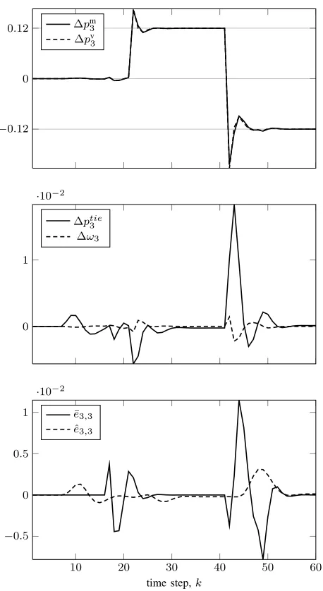
i andξui times the state and input constraints. To intepret these results, consider, for example, area 3:99.1%of the input constraint (on the reference power) is reserved for the main controller, which designs the nominal plan to steer the states to the required steady-state values. Of the remaining0.9%,0.8% is allocated to the ancillary MPC controller, which handles the planned error, while the final 0.1% is required by the robust controller for dealing with unplanned error. The network is subjected to the load power deviation schedule shown in Table III; Figure 2 shows the response for area 3. The area states are shown to settle to steady-state values, while frequencies remain bounded and around zero. Additionally, the planned error is seen to be larger in magnitude than the unplanned error, which justifies the choice of not considering the whole error as unplanned by taking a conventional robust approach.
VI. CONCLUSIONS
This paper has presented a novel DMPC-based approach to automatic generation control in multi-area power systems. The scheme attains desirable guaranteed properties—constraint satisfaction, feasibility and stability—by employing a three-term control law in each area; the first three-term steers states to steady values, the second handles planned disturbances and errors, while the third term robustly rejects unplanned disturbances. The algorithm requires the solution of two MPC problems per area at each time step, albeit the complexity of these is similar to conventional MPC. A detailed off-line design methodology was proposed, and demonstrated on an example 4-area system.
Finally, we remark that the price of obtaining the guarantees of the proposed approach is conservatism: if the inter-area coupling is too strong, then the design procedure will fail and the proposed approach will not be applicable. On the other hand, if the design procedure succeeds then the coupling is sufficiently weak, as was the case in the 4-area system demonstrated in Section V.
REFERENCES
[1] H. Shayegi, H. A. Shayanfar, and A. Jalil, “Load frequency control strategies: A state-of-the-art survey for the researcher,”Energy Conversion and Management, vol. 50, pp. 344–353, 2009.
TABLE III
TIMING,LOCATION AND MAGNITUDE OF LOAD POWER CHANGES,∆pd i.
Time step 5 15 20 40 40
Areai 1 2 3 3 4
∆pd
−0.12 0
0.12 ∆pm3
∆pv 3
0 1
·10−2
∆ptie 3
∆ω3
10 20 30 40 50 60
−0.5 0 0.5 1
·10−2
time step,k
¯
e3,3
ˆ
[image:10.612.51.280.50.469.2]e3,3
Fig. 2. State trajectories of area 3: (top) deviations in mechanical input power (p.u.) and governor output power (p.u.); (middle) deviations in tie-line power (p.u.) and rotor speed (rad s−1); (bottom) planned error and unplanned error
in the third state, mechanical input power∆pm 3.
[2] S. K. Pandey, S. R. Mohanty, and N. Kishor, “A literature survey on load-frequency control for conventional and distribution generation power systems,”Renewable and Sustainable Energy Reviews, vol. 25, pp. 318– 334, 2013.
[3] E. E. Ejegi, J. A. Rossiter, and P. A. Trodden, “A survey of techniques and opportunities in power system automatic generation control,” in Proceedings of the 2014 UKACC International Conference on Control (CONTROL 2014), Jul. 2014, pp. 537–542.
[4] N. Jaleeli, L. S. VanSlyck, D. N. Ewart, L. H. Fink, and A. G. Hoffmann, “Understanding automatic generation control,”IEEE Transactions on Power Systems, vol. 7, no. 3, pp. 1106–1122, Aug 1992.
[5] J. B. Rawlings and B. T. Stewart, “Coordinating multiple optimization-based controllers: New opportunities and challenges,”Journal of Process Control, vol. 18, pp. 839–845, 2008.
[6] S. J. Qin and T. A. Badgwell, “A survey of industrial model predictive control technology,”Control Engineering Practice, vol. 11, pp. 733–764, 2003.
[7] J. B. Rawlings and D. Q. Mayne,Model Predictive Control: Theory and Design. Nob Hill Publishing, 2009.
[8] D. Q. Mayne, “Model predictive control: Recent developments and future promise,”Automatica, vol. 50, pp. 2967–2986, 2014.
[9] R. Scattolini, “Architectures for distributed and hierarchical Model
Predictive Control – A review,”Journal of Process Control, vol. 19, pp. 723–731, 2009.
[10] P. D. Christofides, R. Scattolini, D. Muñoz del la Peña, and J. Liu, “Distributed model predictive control: A tutorial review and future research directions,”Computers & Chemical Engineering, vol. 51, pp. 21–41, 2013.
[11] A. N. Venkat, I. A. Hiskens, J. B. Rawlings, and S. J. Wright, “Distributed MPC strategies with application to power system automatic generation control,”IEEE Transactions on Control Systems Technology, vol. 16, no. 6, pp. 1192–1206, 2008.
[12] E. Camponogara, D. Jia, B. H. Krogh, and S. Talukdar, “Distributed model predictive control,”IEEE Control Systems Magazine, vol. 22, no. 1, pp. 44–52, Feb 2002.
[13] M. Ma, H. Chen, X. Liu, and F. Allgöwer, “Distributed model predictive load frequency control of multi-area interconnected power system,” International Journal of Electrical Power and Energy Systems, vol. 62, pp. 289–298, 2014.
[14] E. E. Ejegi, J. A. Rossiter, and P. A. Trodden, “Distributed load frequency control of a deregulated power system,” in Proceedings of the 2016 UKACC International Conference on Control (CONTROL 2016), 2016. [15] A. Ersdal, L. Imsland, and K. Uhlen, “Model predictive load-frequency control,”IEEE Transactions on Power Systems, vol. 31, no. 1, pp. 777– 785, 2016.
[16] S. Riverso, M. Farina, and G. Ferrari-Trecate, “Plug-and-play decentral-ized model predictive control for linear systems,”IEEE Transactions on Automatic Control, vol. 58, no. 10, pp. 2608–2614, 2013.
[17] R. M. Hermans, A. Joki´c, M. Lazar, A. Alessio, P. P. van den Bosch, I. A. Hiskens, and A. Bemporad, “Assessment of non-centralised model predictive control techniques for electrical power networks,”International Journal of Control, vol. 85, no. 8, pp. 1162–1177, 2012.
[18] S. V. Rakovi´c, E. C. Kerrigan, D. Q. Mayne, and K. I. Kouramas, “Optimized robust control invariance for linear discrete-time systems: Theoretical foundations,”Automatica, vol. 43, no. 5, pp. 831–841, 2007. [19] M. Farina and R. Scattolini, “Distributed predictive control: A non-cooperative algorithm with neighbor-to-neighbor communication for linear systems,”Automatica, vol. 48, pp. 1088–1096, 2012.
[20] S. Riverso and G. Ferrari-Trecate, “Tube-based distributed control of linear constrained systems,”Automatica, vol. 48, pp. 2860–2865, 2012. [21] P. A. Trodden and J. M. Maestre, “Distributed predictive control with minimization of mutual disturbances,”Automatica, vol. 77, pp. 31–43, 2017.
[22] D. Q. Mayne, M. M. Seron, and S. V. Rakovi´c, “Robust model predictive control of constrained linear systems with bounded disturbances,” Automatica, vol. 41, no. 2, pp. 219–224, 2005.
[23] P. Baldivieso, B. Hernandez, and P. Trodden, “Nested dis-tributed model predictive control,” 2016, accepted for 2017 IFAC World Congress, Toulouse, July 2017. Preprint available at
https://arxiv.org/abs/1610.09205.
[24] J. Machowski, J. W. Bialek, and J. R. Bumby,Power System Dynamics: Stability and Control, 2nd ed. John Wiley & Sons, Ltd, 2008. [25] D. DeHaan and M. Guay, “A real-time framework for model-predictive
control of continuous-time nonlinear systems,”IEEE Transactions on Automatic Control, vol. 52, no. 11, pp. 2047–2057, 2007.
[26] G. Pannocchia, J. B. Rawlings, D. Q. Mayne, and G. M. Mancuso, “Whither discrete time model predictive control?”IEEE Transactions on Automatic Control, vol. 60, no. 1, pp. 246–252, 2015.
[27] M. Farina, P. Colaneri, and R. Scattolini, “Block-wise discretization accounting for structural constraints,”Automatica, vol. 49, no. 11, pp. 3411–3417, 2013.
[28] J. M. Maciejowski,Predictive Control with Constraints. Prentice Hall, 2002.
[29] P. B. Monasterios and P. Trodden, “Output feedback quasi-distributed MPC for linear systems coupled via dynamics and constraints,” in Proceedings of the 2016 UKACC International Conference on Control (CONTROL 2016), Aug. 2016.
[30] D. Q. Mayne, S. V. Rakovi´c, R. Findeisen, and F. Allgöwer, “Robust output feedback model predictive control of constrained linear systems,” Automatica, vol. 42, pp. 1217–1222, 2006.
[31] S. V. Rakovi´c and D. Q. Mayne, “Set robust control invariance for linear discrete time systems,” inProceedings of the 44th IEEE Conference on Decision and Control, and the European Control Conference, Dec 2005. [32] S. Riverso and G. Ferrari-Trecate, “HYCON2 benchmark: Power network