This is a repository copy of Correlation of neural activity with behavioral kinematics reveals distinct sensory encoding and evidence accumulation processes during active tactile sensing.
White Rose Research Online URL for this paper: http://eprints.whiterose.ac.uk/129011/
Version: Accepted Version
Article:
Delis, I, Dmochowski, JP, Sajda, P et al. (1 more author) (2018) Correlation of neural activity with behavioral kinematics reveals distinct sensory encoding and evidence
accumulation processes during active tactile sensing. NeuroImage, 175. pp. 12-21. ISSN 1053-8119
https://doi.org/10.1016/j.neuroimage.2018.03.035
Copyright (c) 2018 Elsevier Inc. Licensed under the Creative Commons Attribution-Non Commercial No Derivatives 4.0 International License
(https://creativecommons.org/licenses/by-nc-nd/4.0/).
[email protected] https://eprints.whiterose.ac.uk/ Reuse
This article is distributed under the terms of the Creative Commons Attribution-NonCommercial-NoDerivs (CC BY-NC-ND) licence. This licence only allows you to download this work and share it with others as long as you credit the authors, but you can’t change the article in any way or use it commercially. More
information and the full terms of the licence here: https://creativecommons.org/licenses/
Takedown
If you consider content in White Rose Research Online to be in breach of UK law, please notify us by
Correlation of Neural Activity with Behavioral Kinematics Reveals Distinct Sensory Encoding and Evidence Accumulation Processes During Active Tactile Sensing
Ioannis Delis1, Jacek P. Dmochowskiβ, Paul Sajda1,γ,* and Qi Wang1,*
1Department of Biomedical Engineering, Columbia University, σew York, σY 100β7, USA
βDepartment of Biomedical Engineering, City College of σew York, σew York, σY 100γ1,
USA
γData Science Institute, Columbia University, σew York, σY 100β7, USA
Abstract
Many real-world decisions rely on active sensing, a dynamic process for directing our
sensors (e.g. eyes or fingers) across a stimulus to maximize information gain. Though
ecologically pervasive, limited work has focused on identifying neural correlates of the
active sensing process. In tactile perception, we often make decisions about an
object/surface by actively exploring its shape/texture. Here we investigate the neural
correlates of active tactile decision-making by simultaneously measuring
electroencephalography (EEG) and finger kinematics while subjects interrogated a haptic
surface to make perceptual judgments. Since sensorimotor behavior underlies decision
formation in active sensing tasks, we hypothesized that the neural correlates of
decision-related processes would be detectable by relating active sensing to neural activity. σovel
brain-behavior correlation analysis revealed that three distinct EEG components,
localizing to right-lateralized occipital cortex (LτC), middle frontal gyrus (MFG), and
supplementary motor area (SMA), respectively, were coupled with active sensing as their
activity significantly correlated with finger kinematics. To probe the functional role of these
components, we fit their single-trial-couplings to decision-making performance using a
hierarchical-drift-diffusion-model (HDDM), revealing that the LτC modulated the
encoding of the tactile stimulus whereas the MFG predicted the rate of information
integration towards a choice. Interestingly, the MFG disappeared from components
uncovered from control subjects performing active sensing but not required to make
perceptual decisions. By uncovering the neural correlates of distinct stimulus encoding
and evidence accumulation processes, this study delineated, for the first time, the
Keywords
active tactile sensing, perceptual decision-making, EEG, Pantograph, canonical
correlation analysis, hierarchical drift diffusion model
Highlights
1. Activity in three brain regions was coupled with active tactile sensing kinematics
2. Active touch correlated with visual but not somatosensory cortex activity
3. Brain-behavior correlations accounted for single-trial decision-making
performance
4. V1 and MFG activations predicted non-decision time and drift rate, respectively
1. Introduction
Perceptual decisions rely on the integration of sensory evidence from the
environment (Heekeren et al., 2004; Hanks and Summerfield, 2017). The quality of
sensory evidence depends highly on our actions, as our movements affect how we
sample, process and integrate information from the external world (Najemnik and Geisler,
2005; Renninger et al., 2007; Navalpakkam et al., 2010; Schroeder et al., 2010;
Chukoskie et al., 2013; Toscani et al., 2013; Yang et al., 2016a; Tomassini et al., 2017;
Tomassini and D'Ausilio, 2017). Hence, to optimize the speed and accuracy of our
perceptual decisions we need to direct our actions so as to efficiently gather sensory
information, a process called active sensing (Kleinfeld et al., 2006; Yang et al., 2016b).
Importantly, the processing of sensory information acquired actively and its translation
into perceptual choices requires the interaction of multiple neural processes (and
consequently multiple brain areas) over time (Philiastides and Sajda, 2006, 2007;
Heekeren et al., 2008; Summerfield and de Lange, 2014; Rahnev et al., 2016). However,
despite recent scientific interest in active sensing and decision-making, its neural
underpinnings remain poorly understood.
Here we address this gap using a response-time active tactile decision-making
task in which we simultaneously measured the electroencephalogram (EEG), active
sensing behavior (movement kinematics) and task performance (accuracy and response
time - RT) of subjects, the goal being to uncover the patterns of neural activity and
sensorimotor behavior that drive active perceptual decisions.
To achieve this goal, we proceed in two steps. We first aim to characterize
recorded EEG signals with the behavioral kinematics and extract components of neural
activity coupled with components of sensorimotor behavior. Specifically, we hypothesize
that changes in the speed with which subjects explore the tactile stimulus are indicative
of the strategy they employ for acquiring and accumulating perceptual information and
thus reflect active sensing behavior. Hence, we use the velocity profiles of the finger
movements performed on each trial as correlates of the EEG recordings in order to
uncover the neural underpinnings of active tactile sensing. The main advantage of this
methodology is that it replaces unspecific measures of neural activations with measures
that directly quantify the coupling between the components of continuous finger
movement and brain activity, thereby tapping more directly into the neural correlates of
tactile active exploration.
We further hypothesize that one’s active sensing behavior, and the neural activity
that underlies it, provides a view into the processes leading to decision formation. Thus,
we ask if the perceptual, cognitive and motor processes involved in active tactile
decision-making are modulated by the strength of the identified brain-behavior couplings. To
dissect the constituent processes of decision-making during active sensing we employ a
hierarchical drift diffusion model (HDDM) analysis. To assess if these processes bear any
relation to the extracted brain-behavior correlated components, we integrate the HDDM
with a regression analysis that uses the brain-behavior correlations as predictors for the
HDDM parameters. The HDDM framework therefore provides a principled approach to
investigate whether the neural representations of active tactile sensory processing drive
decision formation and enables one to identify which of its integral processes may be
stimulus encoding and evidence accumulation, are driven by two distinct components of
brain-behavior coupling.
2. Materials and Methods
β.1 Active tactile texture discrimination task. Fifteen healthy right-handed subjects
(6 female, aged β6±β years) performed a two-alternative forced choice (βAFC) texture
discrimination task during which they had to compare the amplitudes of two sinusoidal
textures of the same frequency. All experimental procedures have been reviewed and
approved by the Institutional Review Board (IRB) at Columbia University.
Subjects performed the task using a haptic device, called a Pantograph (Campion
et al., β005; Frissen et al., β01β), which can be judiciously programmed to generate tactile
sensations that resemble exploring real surfaces (see Figure 1A). For this binary discrimination task, the workspace of the Pantograph (of dimensions 110mm x 60mm)
was split into two subspaces (left - L and right - R, 55mm x 60 mm each) and subjects
experienced continuous sinusoidal forces of different amplitudes (but same wavelength
of 10mm) in the two subspaces (Figure 1B). Subjects were asked to report as quickly
and as accurately as possible which of the two subspaces had the higher texture
amplitude. They placed their right index finger on the plate of the Pantograph, which was
hidden behind a black curtain, and were allowed to move it freely in the Pantograph
workspace to explore the textures of both subspaces before reporting their choice by
pressing one of two buttons on a keyboard (left arrow for L, right arrow for R). During the
experiment, the curtain blocked the subjects’ view to their fingers, the subjects had no
choices.
τn each trial, subjects compared between the reference amplitude 1 (presented
either on the left or right subspace) and one of six other amplitude levels (0.5, 0.75, 0.9,
1.1, 1.β5, 1.5). Each subject performed β0 trials for each amplitude level, resulting in β0
trials x 6 amplitudes = 1β0 trials in total. The full experiment was split into γ blocks of 40
trials. τne subject showed poor behavioral performance (accuracy was not significantly
different from chance level) and another subject’s EEG recordings were significantly
contaminated with eye movement artifacts, thus data from these two subjects were
removed from any subsequent analyses. We report results from the remaining 1γ
subjects.
β.β Control experiment. We recruited ten healthy right-handed subjects (4
females, aged β4±β years) that were naïve to the experimental setup and the tactile
discrimination experiment described above, and asked them to participate in a second
experiment. The subjects were asked to actively explore the virtual surface generated by
the Pantograph using their right index finger. During the experiment, the participants
experienced the same tactile stimulation as for the tactile discrimination task, i.e.
continuous sinusoidal forces of different amplitudes in the two subspaces, but, in contrast
to the first experiment, they did not have to make any perceptual choice. Hence, this
control experiment served to compare the EEG and kinematic signals between a
decision-making and a non-decision-making haptic task. It therefore allowed us to
individuate the components of neural activity and active sensing that can be solely
attributed to decision-making behavior.
finger position) and applied forces were measured at a sampling frequency of 1000Hz.
Single-trial movement velocity waveforms were computed using the derivatives of the
recorded position. During performance of the task, we also recorded EEG signals at β048
sampling frequency using a Biosemi EEG system (ActiveTwo AD-box, 64 Ag-AgCl active
electrodes, 10-10 montage). EEG recordings were preprocessed using EEGLab
(Delorme and Makeig, β004) as follows. EEG signals were first down-sampled to 1000Hz
to match movement kinematics and dynamics. Then, they were bandpass filtered to
1-50Hz using a Hamming windowed FIR filter. To isolate the purely neural component of
the EEG data, we used the following procedure: we first reduced the dimensionality of the
EEG data by reconstituting the data using only the top γβ principal components derived
from Principal Component Analysis (PCA). Thereafter, an Independent Component
Analysis (ICA) decomposition of the data was performed using the Infomax algorithm (Bell
and Sejnowski, 1995). We then used an ICA-based artifact removal algorithm called
MARA (Winkler et al., β011) to remove ICs attributed to blinks, horizontal eye movements
(HEτG), muscular activity (EMG), and any loose or highly noisy electrodes. MARA
assigned each IC a probability of being an artifact; we removed components with
probabilities above 0.5.
β.γ EEGβBehaviour analysis. To identify correlations between the EEG recordings
and the subjects’ active sensory experience, we used a novel methodology, termed
EEGβBeh(avior). EEGβBeh extends the previously developed framework StimβEEG
(Dmochowski et al., β017) to make it applicable to simultaneously recorded neural activity
active sensing behavior, but we also note that using finger position yielded qualitatively
very similar results.
The method is based on the temporal filtering of the velocity signals s(t) and the
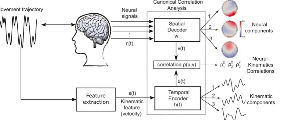
spatial integration of EEG signals recorded from i electrodes (Figure 2):
where * in the first equation denotes convolution between two signals, whereas
the second equation is a weighted summation. The temporal filter h(t) and spatial filter gi
are found by maximizing the correlation between the filtered movement velocity
u(t) and the filtered EEG activity v(t):
To learn the filters that yield maximally correlated EEG and kinematic components,
we performed Canonical Correlation Analysis (Hotelling, 19γ6; De Cheveigne et al., β017)
(CCA), which provides multiple pairs of solutions. Each pair c captures in a spatial
filter of EEG activity and in a temporal filter of the movement velocity. Here we chose
the temporal aperture of the temporal filters to be [-1s,1s] (varying the filter aperture did
not change qualitatively the results). This choice of temporal filter window allowed both
positive and negative lags between the EEG and the velocity signals, which was crucial
for investigating the mutual causal dependencies between the brain and the behavioural
signals. In other words, by allowing the EEG signals to both precede and follow the
velocity signals (within a 1s period), we could identify patterns of brain activity that both
To visualize the spatial distribution of neural activity associated with each filter, we
computed the EEG components using the “forward model” formalism as follows (Parra
et al., β00β; Parra et al., β005; Haufe et al., β014):
where is the autocovariance matrix of the EEG data matrix
and is a matrix containing the C CCA-derived spatial
filters. The corresponding forward models are the columns of matrix .
Hence this approach extracts C pairs of temporal kinematic components and
spatial EEG components ( that correlate with strength in decreasing order
.
To determine statistical significance of the correlations at each learned component
pair ( k > 0), we randomized the phase spectrum of the EEG signals, which disrupted the
temporal relationship between the EEG activity and the kinematics while preserving the
autocorrelation structure of the signals (Theiler et al., 199β). We generated 1000
phase-randomized surrogates of the EEG data and computed EEGβBeh correlations with the
kinematics to define the null distribution from which we estimated p-values. In contrast to
a standard shuffling procedure that disrupts any coordination across EEG sensors, this
phase-randomization procedure maintains the magnitude spectrum of the EEG signals,
thus conserving their autocorrelation structure, which is a fundamental feature of the
original signals when the significance of cross-correlation is assessed. Hence, using this
procedure, the obtained surrogates that define the null distribution are a more plausible
β.4 Source Localization. To identify the brain regions that generated the EEG
component activations we performed a source reconstruction analysis. We used
Brainstorm (Tadel et al., β011), an open-source Matlab package for M/EEG signal
processing, to translate the obtained forward models into distributions of underlying
cortical activity. A standardized head model based on the average template brain of the
Montreal σeurological Institute (MσI) was used as single subject MRI data were not
available. To estimate the sources, we used the whitened and depth-weighted linear
Lβ-minimum norm estimates algorithm with no noise modelling (noise covariance equal to
the identity matrix) and estimated amplitude SσR of the recordings equal to γ (default -
used to compute the regularization parameter). We constrained the orientation of the
source model by modelling at each grid point only one dipole that is oriented normally to
the cortical surface.
β.5 Hierarchical Drift Diffusion Modelling of performance data with EEGβBeh
regressors. We fit the subjects’ performance, i.e. accuracy and response time (RT), with
a hierarchical drift diffusion model (HDDM) (Wabersich and Vandekerckhove, β014) which
assumes a stochastic accumulation of sensory evidence over time, toward one of two
decision boundaries corresponding to correct and incorrect choices (Ratcliff, β00β;
Ratcliff and McKoon, β008; Ratcliff et al., β015; Ratcliff et al., β016). The model returns
estimates of internal components of processing such as the rate of evidence
accumulation (drift rate), the distance between decision boundaries controlling the
amount of evidence required for a decision (decision boundary), a possible bias towards
one of the two choices (starting point) and the duration of non-decision processes
common practice, we assumed that stimulus differences affected the drift rate (Ratcliff
and Frank, β01β).
In short, the model iteratively adjusts the above parameters to maximize the
summed log likelihood of the predicted mean response time (RT) and accuracy. The DDM
parameters were estimated in a hierarchical Bayesian framework, in which prior
distributions of the model parameters were updated on the basis of the likelihood of the
data given the model, to yield posterior distributions (Kruschke, β010b; Wiecki et al.,
β01γ; Wabersich and Vandekerckhove, β014). The use of Bayesian analysis, and
specifically the hierarchical drift diffusion model has several benefits relative to traditional
DDM analysis. First, posterior distributions directly convey the uncertainty associated with
parameter estimates (Gelman, β00γ; Kruschke, β010a). Second, the Bayesian
hierarchical framework has been shown to be especially effective when the number of
observations is low (Ratcliff and Childers, β015). Third and more importantly, this
framework supports the use of other variables as regressors of the model parameters to
assess relations of the model parameters with other physiological or behavioral data
(Cavanagh et al., β011; Cavanagh et al., β014; Frank et al., β015; σunez et al., β015;
Turner et al., β015; Pedersen et al., β016; σunez et al., β017). This property of the HDDM
allowed us to establish the link between the results of the brain-behavior coupling analysis
and the decision parameters of the model.
To implement the hierarchical DDM, we used the JAGS Wiener module (Wabersich
and Vandekerckhove, β014) in JAGS (Plummer, β00γ), via the Matjags interface in Matlab
to estimate posterior distributions. For each trial, the likelihood of accuracy and RT was
model parameters (boundary separation, starting point, non-decision time, and drift rate).
Parameters were drawn from uniformly distributed priors and were estimated with
non-informative mean and standard deviation group priors. The starting point was set as the
midpoint between the two decision boundaries as the experimental design induced no
bias towards one of the two choices (Philiastides et al., β011). There were 5,500 samples
drawn from the posterior; the first 500 were discarded (as “burn-in”) and the rest were
subsampled (“thinned”) by a factor of 50 following the conventional approach to MCMC
sampling whereby initial samples are likely to be unreliable due to the selection of a
random starting point and neighboring samples are likely to be highly correlated (Wiecki
et al., β01γ; Wabersich and Vandekerckhove, β014). The remaining samples constituted
the probability distributions of each estimated parameter.
As part of the model fitting within the HDDM framework, we used the single-trial
EEGβBeh correlations of the identified components as regressors of the decision
parameters (non-decision time, and drift rate, ) as follows:
In these regressions, are the squared single-trial EEGβBeh correlations of the
three components respectively. The coefficients ( ) weight the slope of the
non-decision time (drift rate) by the values of on that specific trial, with an intercept ( ).
By using these eight regression coefficients we were able to test the influences of each
of the three identified components on either of the model parameters (Cavanagh et al.,
β014). Posterior probability densities of each regression coefficient were estimated using
(see Figure 4B-C for examples). Significantly positive (negative) effects were determined
when >99% of the posterior density was higher (lower) than 0.
For comparison with alternate models, we used the Deviance Information Criterion
(DIC), a measure widely used for fit assessment and comparison of hierarchical models
(Spiegelhalter et al., β00β). DIC selects the model that achieves the best trade-off
between goodness-of-fit and model complexity. Lower DIC values favor models with the
highest likelihood and least degrees of freedom.
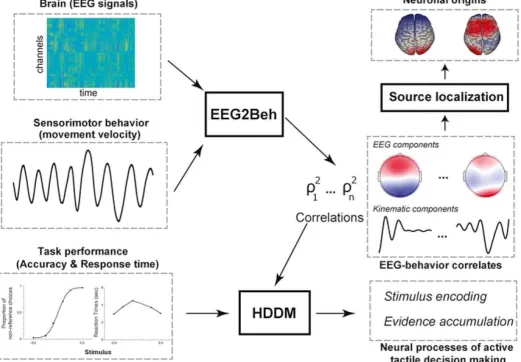
A detailed account of the analysis pipeline implemented in this study is given
graphically in the form of a flowchart in Figure 3.
3. Results
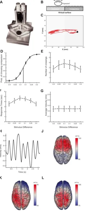
3.1 Tactile discrimination performance. To generate tactile stimulation that can be
actively sensed, we employed a haptic stimulator (Campion et al., 2005; Frissen et al.,
2012) (Figure 1A) and programmed it to render a virtual grating texture with different
amplitudes (Figure 1B). In particular, we split the workspace of the haptic stimulator into
two regions (left - L and right - R) and asked fifteen subjects to actively explore the virtual
surface and report as quickly and as accurately as possible which of the two subspaces
had higher texture amplitude. One of the two regions (termed reference) had a fixed virtual
amplitude while the other subspace (termed comparison) had a varying amplitude for
each trial. On each trial, subjects actively moved their finger to scan the two regions in
order to compare a reference texture amplitude (which was randomly presented in one of
the two regions) and a comparison texture with higher or lower amplitude (six amplitude
improved significantly with increasing stimulus difference, as reflected by a larger fraction
of correct choices (p<10-7, F(2, 36)=27.03) and faster RTs (p<0.05, F(2, 36)=4.04)
(Figure 1D,F).
3.2 Active sensing behavioral kinematics. During this active tactile
decision-making task, we also recorded a) the subjects’ finger position, offering a detailed account
of their active sensing strategy and b) their EEG activity reflecting the neural dynamics
that underlie performance of this task. First, we examined what aspects of the active
sensing strategy used by the subjects were affected by task difficulty. We found that
subjects switched between the two textures (in order to compare their amplitudes before
reaching a decision) more times when the task was harder, but this dependence of the
number of crossings on stimulus differences was not significant at the population level
(p=0.17, F(2,36)=1.87, Figure 1E). Interestingly, the time-averaged speed with which the
subjects scanned the textures was independent of the stimulus difference (Figure 1G).
However, instantaneous finger velocity varied considerably within each trial suggesting
that subjects modulated their tactile exploration speed in order to actively sense the two
surfaces before making a choice (Figure 1H).
3.3. EEG activity. After characterizing the subjects’ active sensing behavior, we
aimed to investigate the structure of their whole-brain activity during performance of this
task. We thus applied Principal Component Analysis (PCA) to the EEG recordings pooled
across all participants to extract the main dimensions of EEG variation and then
performed source localization analysis to the first three PCs to identify the neuronal
origins of these brain activations. We found that the most prominent EEG components
right-lateralized somatosensory as well as other parietal areas (second and third PC,
Figure 1K-L).
3.4 Three distinct brain to active sensing couplings. Following the aforementioned
general characterization of EEG activity in this task, we then probed the relationship
between the subjects’ brain activity and their active sensory experience. We hypothesized
that the subjects’ active sensing strategy is represented by their finger kinematics and in
particular their movement velocity which they varied in order to actively explore the two
surfaces. To relate movement velocity with the recorded EEG signals, we capitalized on
a novel computational approach, termed “Stim2EEG” (Dmochowski et al., 2017), for the
fusion of neuroimaging and dynamic stimulus signals. We extended the applicability of
this approach to sensorimotor behavioral measurements (kinematic signals here) and
termed this analytical method as “EEG2Beh(avior)”. EEG2Beh aims to identify
components of brain – sensorimotor behavior coupling using an optimization procedure
based on Canonical Correlation Analysis (CCA) (Hotelling, 1936). Specifically, EEG2Beh
selects a spatial filter w to apply to the EEG signals and a temporal filter h to apply to the
kinematic feature (i.e. velocity) time series such that the resulting filter outputs are
maximally correlated in time (Figure 2). Ultimately, this approach outputs multiple spatial
EEG components matched with multiple temporal kinematic components as well as the
coefficient of determination (square of the correlation coefficient) of the filter outputs ,
a measure of the brain-behavior coupling for each pair of components.
To identify EEGβBeh components that describe performance of this task
consistently across subjects, we pooled the pre-processed EEG and velocity data across
pairs of distinct EEG (spatial) and kinematic (temporal) components (Figure 2) showing
significant EEGβBeh coupling (p<0.05, corrected for multiple comparisons using
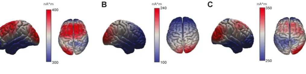
Bonferroni correction). Source localization of the first EEG component revealed a
neuronal origin in the right lateral occipital complex (LτC) (Figure 4A). The brain source
of the second EEG component was localized to the right middle frontal gyrus (MFG)
(Figure 4B), whereas the third component had its origin in the supplementary motor area
(SMA) and premotor cortex (Figure 4C). Interestingly, the first two components with the
highest brain-behavior couplings did not correspond to the EEG components that
accounted for the highest variance in the data (see sources of the three first PCs in Figure
1J). This finding suggests that the components carrying most of the power in the EEG recordings did not correlate with active sensing; instead brain areas with lower activity
(less than 10% of the variance of the EEG data) were more strongly coupled with the
movement kinematics.
To evaluate whether the three extracted EEGβBeh components characterized the
EEG-kinematics relationship for each individual subject, we filtered the single-subject
EEG and velocity signals with the identified spatial and temporal filters respectively and
computed the EEGβBeh correlations of each subject. To test for statistical significance
of the single-subject correlations, we performed a permutation test using
phase-randomized EEG data (see Materials and Methods for details). First, the phase-spectrum
of the EEG time series of each subject was randomized and then the resulting surrogate
EEG data were filtered by the spatial filters before computing the correlations with the
temporally filtered velocity signals. Using this test (repeated 1000 times), we found that
Bonferroni correction) for all but three subjects for each component (different subjects for
each component, so each subject had at least two of the three components), which
suggests that the identified components were present in the majority of the subjects.
3.5 Brain-behavior correlations predict HDDM parameters. Having specified the
main components of brain activity and active sensing behavior that describe this task, we
then aimed to establish the missing link between this brain-behavior coupling and
decision-making performance. We asked whether trial-to-trial fluctuations in the
brain-behavior coupling have a direct influence on brain-behavior and, in particular, which
decision-making processes they may be implicated in. To address this question, we first quantified
the brain-behavior coupling in single trials, i.e. computed single-trial values by filtering
the single-trial EEG and kinematic data with the identified spatial and temporal filters
respectively. Then, we integrated the single-trial values into a hierarchical drift diffusion
model (HDDM) (Ratcliff and McKoon, 2008; Wiecki et al., 2013), a cognitive model of
decision-making behavior that decomposes task performance, i.e. accuracy and RT, into
the internal components of processing representing the rate of sensory information
integration (drift rate, ), the amount of evidence required to make a choice (decision
boundary separation, ), and the duration of other processes (non-decision time, ), i.e.
stimulus encoding and response production.
As part of the fitting of the HDDM model, we estimated regression coefficients ( ,
) to determine the relationship between trial-to-trial variations in and the main
decision parameters. Our hypothesis was that that the strength of the brain-behavior
couplings pertains to decision formation. Hence, this approach served to assess whether
showed any relation to the identified brain-behavior correlations on single trials.
Our results revealed that the task performance data were fit well by the HDDM with
trial-dependent drift rate, non-decision time and decision boundary separation (R2=0.81,
see Figure 5A for the model fits of the behavioral accuracies and RTs). This finding
indicates that the HDDM model can explain behavior during such a task that, in contrast
to most speeded decision-making tasks, includes active sampling and exploration of both
alternatives and consequently longer response times. In particular, we found considerably
longer non-decision times (1.71s±0.01s) than those typically found during rapid
perceptual decisions (0.3s-0.4s), which suggests that these longer non-decision time
durations likely capture the extra time needed to sense both stimuli and switch between
them.
More importantly, the HDDM model with EEG2Beh regressors of the non-decision
times and drift rates, provided a better trade-off between goodness-of-fit and complexity
(as assessed by the Deviance Information Criterion - DIC for model selection
(Spiegelhalter et al., 2002)) compared to alternative HDDM models (see Figure 5 for
DIC comparisons). Specifically, the model of choice (shown in Figure 6A) provided a
better fitting of the task performance data than a) a model that did not include EEG2Beh
regressors, b) models that included regressors of the non-decision times only or the drift
rates only, or c) a model that included a regressor of the decision boundary separation.
Thus, we deduced that using the brain-behavior couplings as predictors of single-trial
non-decision times and drift rates yielded better HDDM model performance.
Central to our study, we then examined whether any of the EEG2Beh regressors
brain-behavior correlations of the first (occipital) component were significantly negatively
correlated to the non-decision times ( 1<0 with p<0.01, i.e. the stronger the coupling the
shorter the non-decision times, Figure 6B) and the correlations of the second (prefrontal)
component were predictive of the drift rate ( 2>0 with p<0.01, i.e. higher drift rates for
stronger couplings, Figure 6C). Interestingly, the estimated effects ( 2) of the of the
second component on drift rate were not significantly different for the three difficulty levels
(Figure 5C) indicating that this relationship is not modulated by the amount of sensory
evidence. In contrast, the constant term ( 0) showed a significant increase (p<0.001) with
the amount of sensory evidence. Taken together, these results suggest that the drift rate
was proportional to the amount of sensory evidence and its trial-to-trial fluctuations were
modulated by the brain-behavior couplings over prefrontal areas. Finally, the third
component showed similar relations to the HDDM parameters as the ones described
above (negative for the non-decision times and positive for the drift rates) but none of the
two were significant (p>0.05).
3.6 No MFG activation when performing active sensing but not decision-making.
To validate the functional roles of the identified components as revealed by the HDDM
analysis, we also applied the EEG2Beh analysis to EEG and kinematic signals recorded
while naïve subjects actively interrogated the same stimuli but did not have to make a
perceptual choice. The obtained neural components localized to SMA (first and third
component) and LOC (all three components, see Figure 7). The presence of these
activations in such a non-decision-making task corroborates their involvement in active
sensing behavior. In particular, these results are consistent with the identified implication
sensory/stimulus-encoding role, and a neither sensory nor decision (but likely a motor) related role for SMA.
Importantly, no MFG activation was found in this control experiment which indicates that
this component is present only when a perceptual choice is made and reflects a
decision-related signal.
4. Discussion
In this study, we probed the components of brain activity and sensorimotor
behavior involved in active perceptual decisions and showed that the sensorimotor
strategy employed for active sensing drives the perceptual and cognitive processes
leading to decision formation. In particular, the quality of tactile stimulus encoding and
evidence accumulation pertains to the coupling between the kinematic patterns of the
subject’s motion and the neural activity that drives (and is driven by) this motion. The
significance of our approach and the implications of the findings are discussed in the
following.
4.1 Active sensing as a window onto the neural processes of decision-making.
There has been significant progress in the study of the neural processes of perceptual
decision-making (Heekeren et al., 2008; Donner et al., 2009; Rushworth et al., 2009;
O'Connell et al., 2012; Wyart et al., 2012; Lou et al., 2014; Hanks and Summerfield,
2017). However, in most decision-making research, sensory information sampling,
processing, and integrating takes place passively, whereas in real-world settings most
perceptual decisions are made during active behaviors (e.g eye movements to gather
information about a visual stimulus (Najemnik and Geisler, 2005; Kleinfeld et al., 2006;
et al., 2013; Toscani et al., 2013) or hand/finger movements to explore a tactile surface
(Lederman and Klatzky, 1986; Lederman and Klatzky, 1987; Oddo et al., 2017; Rongala
et al., 2017)). This process entails the integration of information from multiple locations in
order to both select the next movement and solve the task (Hayhoe and Ballard, 2005;
Rothkopf et al., 2007; Schroeder et al., 2010; Chukoskie et al., 2013; Morillon et al., 2015;
Schroeder and Ritt, 2016; Yang et al., 2016a; Yang et al., 2016b). Here we investigated
this sensorimotor coupling in a decision making task using a novel approach which
decodes a pattern of neural activity that encodes a pattern of the movement kinematics
(Dmochowski et al., 2017). The development of similar approaches relating neural activity
to continuous stimulus or behavioral variables has been a topic of major recent interest
(Crosse et al., 2016; De Cheveigne et al., 2017; Ince et al., 2017; Oddo et al., 2017).
4.2 A distributed neural network for active perceptual decision-making. Here, we
found that movement kinematics are encoded in different brain regions and the respective
brain-behaviour coupling was predictive of dissociable decision-making processes.
First, the coupling of right occipital cortical activity with the movement kinematics
was shown to modulate the non-decision time duration of the decision formation
procedure. This parameter includes the durations of a) the stimulus encoding and b) the
motor response to indicate the choice made. From these two processes, the latter is not
expected to vary significantly from trial to trial in this experimental paradigm and
furthermore, motor actions are not localized in occipital areas. Hence, we deduce that the
correlation of the first pair of EEG2Beh components is likely associated with the stimulus
encoding process. We further discuss the role of visual cortex in tactile decision-making
Second, we found that the component localizing to prefrontal cortex was predictive
of the rate of evidence accumulation towards a tactile decision, which is also compatible
with previous work. The prefrontal cortex has been shown to play an important role in
decision-making and, in particular, it has been implicated in perceptual (but also
economic) information integration (Heekeren et al., 2006; Philiastides et al., 2011;
Rahnev et al., 2016; Sterzer, 2016). We should note that, in this study, the contribution
of prefrontal cortex to evidence accumulation may be direct, i.e. by representing a
decision variable, or indirect, i.e. by playing a role in regulating other cognitive processes
such as task engagement, attention or arousal that impact on the rate at which evidence
is accumulated. Also, our findings do not rule out the possibility that other brain areas –
not directly related to active sensing - may contribute to regulating evidence accumulation
in this task.
We also identified a third component localizing to the supplementary motor area
that showed significant EEG-kinematics coupling but did not correlate with any DDM
model parameter. SMA participates in producing motor behavior and has been previously
demonstrated to be involved in tactile decision-making (Pleger et al., 2006) and, in
particular, to correlate with perceptual sensitivity to tactile roughness (Kim et al., 2015).
SMA has also been implicated in the calculation of motor plans during continuous
movements (Pereira et al., 2017). We thus aim to further elucidate the role of SMA in
active tactile decisions in future work involving simultaneous EEG and fMRI recordings.
Taken together, our results suggest that active perceptual decision-making is
based on the interaction of different neural networks, which have complementary roles in
2007; Heekeren et al., 2008; Mostert et al., 2015; Delis et al., 2016).
4.3 Deciphering the role of visual cortex in tactile decision-making. Our findings
are consistent with prior work associating the lateral occipital cortex with tactile
processing (Sathian, 2005; Zhang et al., 2005; Stilla et al., 2008; Lucan et al., 2010;
Sathian, 2016) and assigning a multimodal role to the visual cortex (Lacey et al., 2007;
Stilla and Sathian, 2008; Lacey and Sathian, 2011, 2012, 2014, 2015; Murray, 2016;
Murray et al., 2016). Importantly, Zangaladze and collaborators demonstrated the causal
involvement of occipital cortex in tactile discrimination performance (Zangaladze et al.,
1999). Here we investigated further its role in tactile behaviors in which decision times
are under subjects' control and showed that occipital cortex contributes to the
transmission of information from the sensory organs to the evidence accumulation
process. In contrast to current belief that visual cortex represents the features of tactile
stimuli that lead to a “tactile object” (tactile features provide explicit information about
shape, orientation etc.) rather than fine grain tactile textures (as in our experiment)
(Zangaladze et al., 1999), our data showed that the representation of the fine tactile
textures indeed localized to visual cortex.
So why do we see visual cortex in a fine grain tactile discrimination task? We
believe that the difference is due to active sensing. Previous work referenced above used
very controlled, short trial-based paradigms where subjects were presented with stimuli
without a need to actively sense. What is unique to our work is that the process of active
sensing likely results in subjects dynamically forming a representation of the tactile
surface into an object. For example, as they move their finger, exploring the fine texture
textural boundaries and the spatial extent of the textures themselves. Though subjects
do not need to report those object-related properties here, having a representation of
such properties enables them to potentially make more efficient decisions — e.g. using a
representation of the tactile boundary to guide rapid comparisons of textural differences.
Though additional experiments are needed to investigate the interaction of the
representation and the task objective (textural decision vs. object-level decision), our
current work provides evidence that active sensing itself allows the brain to take simple
stimuli and tasks and build more complex representations that would be of greater utility
than just solving the simple task at hand.
4.4 Informed cognitive modeling to uncover latent neural processes. An important
contribution of our study is the dissociation of the roles of the identified neural/kinematic
patterns. This was only made possible by the joint cognitive modeling of behavioral and
neural/kinematic data that linked the neural correlates of sensori-motor behavior with the
cognitive processes involved in decision-making. Similar model-based cognitive
neuroscience approaches have been proposed recently and have been shown to be
effective in characterizing the neural underpinnings of behavioral components (Turner et
al., 2015; Turner et al., 2017). By means of this approach, neural and other physiological
measures of various cognitive processes have been identified (Ratcliff et al., 2009;
Cavanagh et al., 2011; Ratcliff and Frank, 2012; Cavanagh et al., 2014; Dmochowski and
Norcia, 2015; Frank et al., 2015; Nunez et al., 2017). Here we asked whether the neural
representations of active sensing are used to generate decision-making behavior and in
particular if their trial-to-trial fluctuations affect decision-making performance. We found
prefrontal cortices – indexes the efficiency of a) stimulus encoding and b) integration of
perceptual information respectively.
Overall, this study indicates that active sensing provides a window into
understanding the patterns of brain activity and sensorimotor behavior that drive
perceptual decision-making and offers the first direct evidence on the neural networks
underlying active tactile decisions. In particular, we demonstrate that, during active tactile
sensing, the right occipital (presumably “visual”) cortex has a central role in forming tactile
stimulus representations whereas the middle frontal gyrus contributes to regulating how
quickly perceptual evidence accumulates towards a choice.
Figure Captions
Figure1. Experimental design, behavioral results and principal components of EEG signals. A. The Pantograph is a haptic device used to render virtual surfaces that can be
actively sensed. B. The stimulus. We programmed the Pantograph to generate a virtual
grating texture. The workspace was split into two subspaces (left - L and right - R) that
differed in the amplitude of the virtual surface that the subjects actively sensed. τne of
the two sides (randomly assigned) had the reference amplitude (equal to 1) and the other
had the comparison amplitude that varied on each trial taking one of the values: 0.5, 0.75,
0.9, 1.1, 1.β5, and 1.5. C. Index finger trajectory indicating the scanning pattern of the
virtual texture in one trial. The two red dots indicate the starting point and endpoint. τn
this trial, the subject actively sensed the left subspace first, then moved to the right
subspace and explored it before coming back to the left subspace again and reporting
for all stimulus differences. Dots indicate average proportion of choices across subjects
and errorbars are standard error of the means (sem) across subjects. Data are fit using
a cumulative Gaussian function. E. Response times for all stimulus differences shown as
averages (± sem) across subjects. F. σumber of crossings (i.e. switchings between the
two stimuli) for all stimulus differences shown as averages (± sem) across subjects. G.
Average finger velocities for all stimulus differences shown as averages (± sem) across
subjects. H. Velocity profile of the finger movement during the example trial. J-K-L. Brain
sources of the first three principal components of the recorded EEG signals across
subjects.
Figure2. Schematic view of EEGβBeh(avior) and the identified . Subjects move their fingers to actively sense a surface while their brain activity (e.g. EEG signals) ri(t) is
recorded. The relevant kinematic features of the sensorimotor behavior (the movement
velocity here) are extracted, resulting in a time series s(t). An optimization procedure,
implemented via canonical correlation analysis, then computes spatial filters w to apply
to the neural signals and temporal filters h(t) to apply to the velocity such that the resulting
filter outputs are maximally correlated in time. The algorithm output is a set of multiple
EEG-kinematic components and their coupling strengths β. Three pairs of EEG
components (scalp maps of neural activity) and their matching kinematic components
(temporal profiles of velocity filters) were found to show significant correlations.
Figure3. Illustration of the analysis framework implemented in this study. To characterize active tactile decision-making, three types of measurements are simultaneously made: a)
EEG recordings, b) sensorimotor signals (movement kinematics), and c) task
are input to the EEGβBeh algorithm that outputs pairs of brain – behavior coupling
components (scalp maps and temporal kinematic filters) and their correlation measures
β. The brain (EEG) components are input to a source localization algorithm to identify
their neuronal origins. The EEGβBeh coupling strengths β inform the hierarchical drift
diffusion modelling (HDDM) of the task performance data. HDDM uses the β to translate
accuracy and RT into the components of decision-making processing (such as evidence
accumulation or stimulus encoding) thereby characterizing the functional role of each
EEGβBeh component.
Figure4. Brain sources of the three EEG components showing significant brain-behavior couplings.
Figure5. HDDM fitting and model comparisons. . Choice proportions and RT distributions are captured by EEGβBeh-informed HDDM. Behavioral RT distributions (in
green) are shown for each stimulus difference together with posterior predictive
simulations from the HDDM (in blue). σegative values in the time axis correspond to
incorrect choices and positive values represent correct choices. Higher histogram values
in the positive time axis indicate higher proportion of correct choices. Fitting accuracy is
worse with lower stimulus differences. B. Comparison with alternate models. We
compared the HDDM model of choice with alternative HDDM models using the Deviance
Information Criterion (DIC). We tested HDDM models where either the drift rate ( ) or the
non-decision time ( ) or both were not dependent on the EEGβBeh correlations and a
model where the decision boundary ( ) was dependent on the EEGβBeh correlations.
Positive difference DIC values (DICmodel – DICoptimal) for all four models indicate that
free parameters.
Figure6. Formulation of best HDDM model and regression results. A. Graphical model showing hierarchical estimation of Drift Diffusion Model parameters with EEGβBeh
regressors. Round nodes represent continuous random variables and double-bordered
nodes represent deterministic variables, defined in terms of other variables. Shaded
nodes represent recorded or computed signals, including single-trial behavioral data
(accuracy, RT) and EEGβBeh coupling measures ( β). τpen nodes represent
unobserved latent parameters. Parameters are modelled as random variables with
inferred means and variances β. Plates denote that multiple random variables share
the same parents and children. The outer plate is over difficulty levels d while the inner
plate is over trials n. For example, each single-trial boundary separation an,d shares the
same parents and β that define the distribution across trials and difficulty levels.
Single-trial variations of non-decision time and drift rate are determined by EEGβBeh
couplings with regression coefficients i and i. B. Violin plots showing the distribution of
the regression coefficients i (100 samples drawn from the distribution) of the coupling
strengths iβ of the three EEGβBeh components for the prediction of single-trial
non-decision times . C. Violin plots showing the distribution of the regression coefficients i
(100 samples drawn from the distribution) of the coupling strengths iβ of the three
EEGβBeh components for the prediction of single-trial drift rates .
Figure7. Brain sources of the three significant EEGβBeh components extracted from the data of the control experiment, i.e. when subjects actively explored the tactile stimuli but
Acknowledgements: This work was supported by the σational Institutes of Health under Grant R01-MH08509β, the U.S. Army Research Laboratory under Cooperative
Agreement W911σF-10-β-00ββ and the UK Economic and Social Research Council
under grant number ES/ L01β995/1 to P.S., and a σARSAD Young Investigator award to
Q.W.. The views and conclusions contained in this document are those of the authors and
should not be interpreted as representing the official policies, either expressed or implied,
of the US Government. The US Government is authorized to reproduce and distribute
reprints for Government purposes notwithstanding any copyright notation herein.
References
B AJ S TJ A
N C
C G W Q H V T P M II A I R
I C I R S V
C JF W TV K A F MJ E
J G
C JF W TV C MX F CM S J S SJ F MJ S
N N
C L S J M MC K RJ S TJ L
P N A S U S A S
C MJ D L GM B A L EC T M T R F TRF
T A MATLAB T R N S C S F H
N
D C A W D D L GM H J S M L EC D
R
D I O A S PG P S P MG S
M EEG N I
D A M S EEGLAB EEG
J N M
D JP N AM C C R T P D
H PL S O
D JP K JJ D G P S P P LC E
N I
D TH S M F P E AK B
C B
J N
F I ) M C G H V G C T
A P A
G A A B I S
R
H TD S C P D M R M H N
H S M F G K D S H JD B B B F O
N I
H M B D E T C S
H HR M S U LG T
N R N
H HR M S B PA U LG A
N
H HR M S R DA B PA U LG I
P N A S USA
H H R B
I RA G BL K C R GA G J S PG A
H
B M
K J C YG P JY C SC W C B HH K SP D A
S M C C P S T R P O
K D A E D ME A
C O N
K JK W B T C S
K JK B W C S
L S S K M
P B R
L S S K R O F V T I T N B
M P M MM W MT B R FL
L S S K V
F
L S S K C M I V T
S
L S C C S K V
P
L S K RL E H M O P B P S
L SJ K RL H M W H O R C
L B L Y P MG S P P
N I
L JN F JJ G R M S K M S T
M B H TA K Y S CE P
C O N
M P K P L FP D
S
M M T I J P
M MM T A T G R V M R M PJ T
N
N J G WS O N
N J G WS E
J V
N V K C R A P P O
P N A S U S A
N MD S R V J I
F
N MD V J S R H
S EEG J M
P
O C RG D PM K SP A
N N
O CM M A S A E JMD M H B F C D M S J H
A
S
P L A C T A P B Y N O A S P L
N
P LC S CD G AD S P R EEG N I
P ML F MJ B G T
P
P M S A M JDR A M C A C S
N
P MG S P T
C C
P MG S P EEG MRI
J N
P MG R R S P N
J N
P MG A R H HR B F C
C B
P B R CC B F B S W K S KE C A F KJ D RJ
N J N
P EJ N SM V K D DI P SE W ME E
D MRI J
N
P M JAGS A B G I
I W D S C
R D N DE R J L AS D E M C
R R A
F P
R R M K G T T
N C
R R F MJ R
N C
R R C R I D F M T C D M
D M D
R R P MG S P Q
EEG P N A S U S A
R R S PL M K G M R R T A D W
D M C D P S
R R S PL B SD M K G D D M C I H
T C S
R LW V P C J W E
J V
R UB M A O CM N A T C N
T I T N N L
R CA B DH H MM T J V
R MFS M RB S C G C
O N
S K V
D
S K A J N
S CE W DA R T S H L P D A S
C O N
S JB R JT S
J N
S DJ B NG C BR L A B
J R S S B
S P M P N A S U S A
S R S K S H B M
S R H R H X M E D G S K N
J V
S C L FP E
N R N
T F B S M JC P D L RM B
MEG EEG C
T J E S L A G B F JD T N T S
M S D P D
T A D A A P
J N
T A A L M WP M E T
L
P N A S U S A
T BM M L F BU I C A T N
T N D D M P R
T BM F BU L BC P TJ V M L A
J M P
W D V J E JAGS A JAGS
B R M
W TV S I F MJ HDDM H B D D M
P F
W I H S T M A ICA
EEG B BBF
W V G V S J S C R
N
Y SC L M W DM A L
Y SCH W DM L M T C O B S
) A E CM G ST S K I
N
) M M E S R S M M H H X S K T
error of the means (sem) across subjects. Data are fit using a cumulative Gaussian function. E. Response times for all stimulus differences shown as averages (±sem) across subjects. F. Number of crossings (i.e. switchings between the two stimuli) for all stimulus differences shown as averages (±sem) across subjects. G. Average finger velocities for all stimulus differences shown as averages (±sem) across subjects. H. Velocity profile of the finger movement during the example trial. J-K-L. Brain sources of the first three principal components of the recorded EEG signals across subjects. (For interpretation of the references to colour in this figure legend, the reader is referred to the Web version of this article.)
Fig. 2. Schematic view of EEG2Beh(avior) and the identified. Subjects move their fingers to actively sense a surface while their brain activity (e.g. EEG signals) ri(t) is recorded. The relevant kinematic features of the sensorimotor behavior (the movement velocity here) are extracted, resulting in a time series s(t). An optimization procedure, implemented via canonical correlation analysis, then computes spatial filters w to apply to the neural signals and temporal filters h(t) to apply to the velocity such that the resulting filter outputs are maximally correlated in time. The algorithm output is a set of multiple EEG-kinematic components and their coupling strengths ρ2. Three pairs of EEG components (scalp maps of neural activity) and their matching kinematic
Fig. 3. Illustration of the analysis framework implemented in this study. To characterize active tactile decision-making, three types of measurements are simultaneously made: a) EEG recordings, b) sensorimotor signals (movement kinematics), and c) task performance measures (accuracy and response time - RT). EEG and kinematic signals are input to the EEG2Beh algorithm that outputs pairs of brain behavior coupling components (scalp maps and temporal kinematic filters) and their correlation measures ρ2. The brain (EEG) components are input to a source localization
algorithm to identify their neuronal origins. The EEG2Beh coupling strengths ρ2 inform the hierarchical drift diffusion modelling (HDDM) of the task performancedata. HDDM uses the ρ2 to
translate accuracy and RT into the components of decision-making processing (such as evidence accumulation or stimulus encoding) thereby characterizing the functional role of each EEG2Beh component.
[image:38.595.38.561.504.621.2]Fig. 5. HDDM fitting and model comparisons. Α. Choice proportions and RT distributions are captured by EEG2Beh-informed HDDM. Behavioral RT distributions (in green) are shown for each stimulus difference together with posterior predictive simulations from the HDDM (in blue). Negative values in the time axis correspond to incorrect choices and positive values represent correct choices. Higher histogram values in the positive time axis indicate higher proportion of correct choices. Fitting accuracy is worse with lower stimulus differences. B.
Comparison with alternate models. We compared the HDDM model of choice with alternative HDDM models using the Deviance Information Criterion (DIC). We tested HDDM models where either the drift rate (δ) or the non-decision time (τ) or both were not dependent on the EEG2Beh correlations and a model where the decision boundary (α) was dependent on the EEG2Beh correlations. Positive difference DIC values (DICmodel DICoptimal) for all four models indicate that the model of choice achieved a better trade-off between goodness-of-fit and number of free parameters. (For interpretation of the references to colour in this figure legend, the reader is referred to the Web version of this article.)
Fig. 6. Formulation of best HDDM model and regression results. A. Graphical model showing hierarchical estimation of Drift Diffusion Model parameters with EEG2Beh regressors. Round nodes represent continuous random variables and double-bordered nodes represent deterministic variables, defined in terms of other variables. Shaded nodes represent recorded or computed signals, including single-trial behavioral data (accuracy, RT) and EEG2Beh coupling measures (ρ2). Open nodes represent unobserved latent parameters. Parameters are modelled as random variables with inferred means μ and variances σ2. Plates denote that multiple random variables share the same parents and children. The outer plate is over difficulty levels d while the inner plate is over trials n.
For example, each single-trial boundary separation an,d shares the same parents μα and σα2 that define the distribution across trials and difficulty levels. Single-trial variations of non-decision time τ
and drift rate δ are determined by EEG2Beh couplings with regression coefficients βi and γi. B. Violin plots showing the distribution of the regression coefficients βi (100 samples drawn from the
[image:39.595.39.562.279.544.2]