White Rose Research Online URL for this paper: http://eprints.whiterose.ac.uk/141998/
Version: Published Version
Article:
Gardner, P., Rogers, T.J., Lord, C. orcid.org/0000-0002-2470-098X et al. (1 more author) (2018) Sparse Gaussian Process Emulators for surrogate design modelling. Applied Mechanics and Materials, 885. pp. 18-31. ISSN 1660-9336
https://doi.org/10.4028/www.scientific.net/amm.885.18
[email protected] https://eprints.whiterose.ac.uk/
Reuse
This article is distributed under the terms of the Creative Commons Attribution (CC BY) licence. This licence allows you to distribute, remix, tweak, and build upon the work, even commercially, as long as you credit the authors for the original work. More information and the full terms of the licence here:
https://creativecommons.org/licenses/
Takedown
If you consider content in White Rose Research Online to be in breach of UK law, please notify us by
Sparse Gaussian Process Emulators
for Surrogate Design Modelling
Paul Gardner
1,a, Timothy J. Rogers
1,b, Charles Lord
1,c,
and Robert J. Barthorpe
1,dDynamics Research Group, Department of Mechanical Engineering, University of Sheffield, Sheffield, UK
a[email protected],b[email protected],c[email protected], [email protected]
Keywords:Gaussian Process, Sparse Gaussian Process, Kriging, Emulator, Surrogate Modelling.
Abstract.Efficient surrogate modelling of computer models (herein defined as simulators) becomes of increasing importance as more complex simulators and non-deterministic methods, such as Monte Carlo simulations, are utilised. This is especially true in large multidimensional design spaces. In order for these technologies to be feasible in an early design stage context, the surrogate model (or emulator) must create an accurate prediction of the simulator in the proposed design space. Gaussian Processes (GPs) are a powerful non-parametric Bayesian approach that can be used as emulators. The probabilistic framework means that predictive distributions are inferred, providing an understanding of the uncertainty introduced by replacing the simulator with an emulator, known as code uncertainty. An issue with GPs is that they have a computational complexity ofO(N3
)(whereNis the number of data
points), which can be reduced toO(N M2
)by using various sparse approximations, calculated from a subset of inducing points (whereM is the number of inducing points). This paper explores the use of
sparse Gaussian process emulators as a computationally efficient method for creating surrogate models of structural dynamics simulators. Discussions on the performance of these methods are presented along with comments regarding key applications to the early design stage.
Introduction
Computer models (simulators) are a vital tool in exploring engineering design options. Often design engineers want to investigate numerous different parameter choices in order to find optimal solutions. These design spaces are often large and multidimensional, meaning that evaluation of the simulator at all parameter combinations of interest is infeasible. In order to reduce the computational load of running numerous simulator evaluations at all parameter combinations of interest, an emulator can be used. An emulator is a fast surrogate model of the computationally expensive simulator that allows accurate interpolation of the design space whilst requiring minimal simulator runs. A common ap-proach for constructing an emulator is to fit a Gaussian process (GP) regression model to simulator evaluations at a small number of predefined inputs in order to learn the simulator’s input to output mapping [1,2]. Optimisation techniques and uncertainty quantification approaches often involve mul-tiple evaluations of the simulator. An emulator provides significant computational savings in being able to interpolate across the design space with reduced computational complexity. As a result, more complex computer models, optimisation or uncertainty quantification techniques become practicable. An additional strength of this approach is the statistical framework of a GP emulator, which pro-vides an assessment of code uncertainty [3] — uncertainty introduced by approximating the simulator with an emulator. The code uncertainty can also be included within an optimisation setting by using a Bayesian optimisation approach [4, 5]; or in a calibration setting with methods such as Bayesian history matching [6, 7]. The inclusion of code uncertainty means that parts of the input space are not excluded or misrepresented when the emulator is uncertain about the prediction of the simulator.
GPs are a popular method for non-parametric, non-linear, Bayesian regression [8, 9]. An issue with GP regression is that training costs O(N3
) (for N observations) with prediction of the mean
and variance costing bothO(N)andO(N2
)respectively [10–12]. Although substantially more com-putationally efficient than running a simulator, this time complexity can make GPs comcom-putationally demanding in circumstances whereN is significantly large. To reduce the computational load, sparse
approximations of the full GP have been developed over recent years; these have been constructed from a regression standpoint [10,12–16]. These sparse approximations reduce the computational com-plexity of training toO(N M2
)[10–12] whereM ≪N andM is a smaller number of inducing points
— a set of pseudo-inputs and their latent function evaluations that are independent from the training data. This paper presents the application of state-of-the-art sparse GP approximations in the context of creating emulators of complex computer models and discusses both model and posterior based ap-proximations and considerations for emulation. The paper outline is as follows: an overview of GP regression is presented, in the following section sparse GP approximations are outlined with discus-sion on model and posterior approximations as well as implications for emulation. Lastly concludiscus-sions are presented highlighting areas of further research.
Gaussian Process Regression
A simulator can be represented by an underlying functional mapping f between a set of inputs X
and their corresponding outputsY = f(X). It may be possible to run the simulator at any arbitrary
set of inputs, however, to evaluate all the combinations of interest is assumed to be computationally expensive; for this reason, only a finite set ofN simulator runs are often available. The objective of
creating an emulator is to reproduce the functional mapping, via regression, so that predictions of the outputs can be made given new inputs. Even though in this paper it is assumed that the simulator is deterministic, a probabilistic approach is useful as the predictive distributions quantify the uncertainty associated with the prediction, known as code uncertainty [3]. A probabilistic framework means that the mapping between a set ofN inputsX ={xn}Nn=1of dimensionDand their corresponding outputs y = {yn}Nn=1 is modelled as p(y|f, X,θ); where θ is a small set of hyperparameters. For a GP
emulator the latent function f is modelled with a GP prior, and the simulator outputs for different
inputs are modelled as jointly Gaussian distributed. The GP prior is formulated as presented in Eq. 1.
p(f|X,θ)∼ N(m, K) (1)
Wheremis a mean function of the formh′(x)β whereh′(x)is a design matrix andβ the
cor-responding hyperparameters. The covariance matrixK defines the prior assumption of the functions
smoothness and is formed from the covariance function whereKij = k(xi, xj), which is dependent
on the hyperparametersθk={σ 2 f, ψ}(σ
2
f is called the signal variance andψare some parameters that
are dependent on the choice of covariance function). The covariance function describes the correla-tion between any two points in the input space via a reproducing kernel Hilbert space. An example covariance function is the squared exponential defined in Eqn. 2.
K =σf2exp((−X−X′)ψ(X−X′)T) (2)
A GP depends on a small number of hyperparameters collectively defined asθ = {β,θk}. The
joint prior between the latent function values (for training f and testing f∗) at training and testing
inputs,XandX∗respectively, can be formed as in Eqn. 3; this uses the definition that a GP is collection
of random variables where a finite set has a joint Gaussian distribution1.
1For compactnessm
ais the mean function relating to the latent functionaandKa,bis the covariance matrix between
[ f f∗ ] ∼ N ([ mf m∗ ] , [
Kf,f Kf,∗
K∗,f K∗,∗
])
(3)
The likelihood for the GP emulator is typically modelled as Gaussian, however the variance term of the likelihood is debated. It is common for a GP emulator to assume that the observations are ‘noise-free’, i.e. repeats at the same set of inputs will always result in the same output — for a deterministic simulator. Even so, due to numerical instabilities in inverting the covariance matrix, GP regression becomes impractical unless a nugget term is added; usually a fixed small number to the diagonal of the covariance matrix. This can be seen as equivalent to assuming a small level of Gaussian white noise on the observation, as assumed in many other fields such as kriging and general regression [9,17] where the likelihood is formed asp(y|f) =N(f, σ2
nI); whereσ 2
nis the variance associated
with the noise. The inclusion of the nugget is known to sometimes lead to inference of the latent functionf that smooths through data points with a variance rather than fitting known input, output
pairs exactly. Andrianakis and Challenor proposed a penalty to the marginal likelihood in order to force a GP emulator with a nugget term to fitting known data points exactly [18]. In this paper a nugget term will be included and assumed to take a very small value. The resulting likelihood is of the formp(y|f) =N (f, νI); whereνis the nugget term.
In order to perform inference the joint prior is combined with the likelihood to form the joint posterior p(f,f∗|y,θ) using Bayes rule (the inputs are dropped for simplicity of notation). The latent training function f can then be marginalised out form the posterior shown in Eqn. 4; this is
possible in closed form due to the Gaussian assumptions.
p(f∗|y,θ) = N(
m∗+K∗,f(Kf,f +νI)− 1
(y−m), K∗,∗−K∗,f(Kf,f +νI)− 1
Kf,∗
)
(4) A fully Bayesian analysis would then require marginalising out the hyperparameters θ, this is
possible forβ and the signal varianceσ2
f [19], but is intractable for the parametersψ. If an MCMC
solution to the hyperparameters is used then this marginalisation provides valuable computational savings. On the other hand if a maximum likelihood approach is used, the computational savings of the marginalisation are minimal as this becomes the optimisation of a small number of parameters. In this paper, a maximum likelihood approach is used due to it being a fast and efficient form of inference with the only negative being that the posterior variance of the GP is slightly underestimated. Inference of the hyperparameters using a maximum likelihood approach requires forming the marginal likelihood, the integral of the prior multiplied by the likelihood, the log form of which is shown in Eqn. 5.
logp(y|X,θ) =−1
2log|Kf,f +νI| − 1
2(y−mf)
T
(Kf,f +νI)− 1
(y−mf)−
N
2 log2π (5) The problem with Eqn. 4 and Eqn. 5 is their dependence on inverting anN ×N matrix requiring
O(N3
)operations [10–12]. If a computationally efficient algorithm is used, the prediction complex-ity of Eqn. 4 is only O(N)with the variance beingO(N2). In order to improve this computational
Sparse GP Approximations
Sparse GP approximations seek to reduce the computational load involved in inverting Kf,f. The
simplest and most naive approach is to select a subset of data (SoD) of size Qfrom the full training
data set (of sizeN whereQ ≪ N) in order to scale down the time complexity toO(Q3
)[10]. The problem is difficult as it relies on a known redundancy within the original data set, which is often not the case — especially in expensive evaluations of a simulator. This loss of information is generally unacceptable in an emulation context, as any simulator runs are expected to have come at a large computational cost. An alternative to SoD is the local GP approach [11]. A simple implementation of local GPs is to divide a data set into equal block sizes of sizeB and fit a GP to each block; reducing
the computational complexity to O(N B2). An issue with the technique is that discontinuities will
occur between each data block, this is often unacceptable in emulators due to their primary use in optimisation or calibration. A less naive implementation of the local GP approach is to use a clustering algorithm to categorise the data into various subsets and fit GP models to each subset of data. As a consequence, the computational complexity of the method will not only be dominated by the largest subset, but will also incur the additional cost of the clustering algorithm. Both SoD and local GP approaches are therefore not ideal for an emulator setting.
This paper explores two key ideas in the generation of sparse GP approximations; approximating the model or the posterior. The techniques use inducing inputs [10] (originally referred to as ‘pseudo-inputs’ [13])Z ={zm}Mn=1, that have a latent function outputu, known as inducing variables in order
to produce sparsity.
Model Approximation Approaches. Quiñonero-Candela and Rasmussen present a unified frame-work for model approximations [10]. These approaches seek to modify the joint prior p(f∗,f) of the GP (Eqn. 3) in order to replace the complexity of invertingKf,f with a less expensive inversion.
This is performed by incorporating inducing points{Z,u}(whereZ are a set of inducing inputs and
u are the corresponding latent function evaluations) into the joint priorp(f∗,f,u) and marginalis-ing the inducmarginalis-ing variables,u, out of the posterior (althoughZ will affect the final solution). The key
assumption for these sparse methods is that the joint prior can be approximated by assuming condi-tional independence betweenf∗ andf givenu. This means thatf∗ andf are only linked throughu;
demonstrated in Eqn. 6.
p(f∗,f)≃q(f∗,f) =
∫
p(f∗|u)q(f|u)p(u)du (6)
Wherep(u) = N(0, Ku,u)is the prior2for the latent variablesuand the test conditional,p(f∗|u),
is defined in Eqn. 7.
p(f∗|u) =N(
K∗,uK− 1
u,uu, K∗,∗−Q∗,∗
)
(7)
It is noted that the notationQa,b=Ka,uKu,u−1Ku,bis used in this paper. The two model
approxima-tion methods detailed in this paper differ in their assumpapproxima-tion about the training condiapproxima-tionalq(f |u),
whilst assuming the same prior for the inducing variables and likelihood.
The assumptions for the training conditionalq(f |u), and the marginalised joint priorp(f∗,f),
for both a deterministic training conditional (DTC) and fully independent training conditional (FITC) approximation are shown in Table 1. The main difference between DTC and FITC is clear in the joint prior, presented in Table 1. The top left corner of the covariance is modified in FITC so that the
2It is common for a nugget,ϵIto be incorporated here [20] for the same reasons as outline for emulators previously, i.e. increases the stability of the inversion of the covariance matrix. A nugget is used in this paper meaning
approximation includes the exact covariance on the diagonal. This transforms the training conditional from deterministic to fully independent.
The posteriorsq(f∗|y,θ)and log marginal likelihoodsp(y|X)for the DTC and FITC approx-imations can be unified into the analytical form outlined in Eqn. 8 and Eqn. 9. [12].
q(f∗|y,θ) =N(
Q∗,fK¯− 1
f,fy, K∗,∗−Q∗,fK¯− 1 f,fQf,∗
)
[image:6.595.69.536.270.435.2](8)
Table 1: DTC and FITC assumptions for the training conditionalq(f|u)and the joint priorp(f∗,f) (where diag[A]refers to the diagonal of matrixA). The joint priorp(f,f∗)is calculated by substi-tuting the training conditionq(f|u)into Eqn. 6 and solving the integral which can be done in closed form.
Method Training Conditional,q(f|u) Joint Prior,p(f∗,f)
DTC N(
Kf,uK− 1 u,uu,0
)
N
(
0,
[
Qf,f Qf,∗
Q∗,f K∗,∗ ])
FITC N(
Kf,uKu,u−1u,diag[Kf,f −Qf,f]
)
N
(
0, [
Qf,f −diag[Qf,f −Kf,f] Qf,∗
Q∗,f K∗,∗
])
logp(y|X) = −1
2log|K¯f,f| − 1 2y
TK¯−1 f,fy−
N
2 log2π (9)
WhereK¯f,f = Qf,f +diag[α(Kf,f −Qf,f)] +νI. The marginal likelihood and posterior of the two methods can be formulated by setting α to zero or one for the DTC and FITC approximations
[image:6.595.127.461.503.754.2]respectively. After settingα, the low rank structure ofK¯f,f should be exploited using the Woodbury
inversion and determinant lemmas in order to improve the computational efficiency. These amend-ments reduce the computational complexity for training toO(N M2
)and for prediction toO(M)and O(M2
)for the mean and variance respectively [10–12].
The question remains of how to set the inducing inputs. One approach is to consider the inducing inputs as a subset of the input data. This poses challenges when global prediction quality is required as the selection of inducing inputs from a discrete set of data will involve some form of greedy or combinatorial optimisation. In contrast, the inducing inputs can be considered to be drawn from any point on the real line leading to a continuous optimisation problem [13]. This allows the inducing inputs to be inferred via optimisation of the log marginal likelihood. When the inducing inputs are equal to the training inputs, the marginal likelihood and the posterior are the same as the full GP for both DTC and FITC. A key drawback of model approximation methods are that optimising via the approximate marginal likelihood means treating the inducing inputs as parameters of the model, adding all the problems of overfitting and optimisation that are evident in parametric models [12,14]. This view of the inducing points means the assumptions about the data and inference approximations are coupled. Learning via the exact marginal likelihood of the approximate model also means that the hyperparameters will be optimal for the approximate model and not necessarily the full GP.
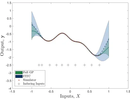
Figure 1 and Fig. 2 present univariate numerical examples where the simulator output is a sample from GP process (a random seed integer of 5 is used in MATLAB) with zero mean and a squared exponential covariance; σ2
f = 1 and ψ = 8. The examples demonstrate the difference in the two
approaches when the hyperparametersθand inducing inputsZ are learnt through optimising the log
marginal likelihood logp(y|X)(Eqn. 9). These illustrate a comparison of the two sparse GP methods, DTC and FITC, with a full GP solution and the training data, where the mean and ±3σ confidence
intervals are displayed for the full and sparse GPs (indicated by the shaded regions). It is shown that FITC gives a better approximation of the variance than DTC, that tends to overestimate (due to the deterministic assumption). Signs of overfitting are present in both methods. In Fig. 1 the variance for DTC whenX ≈ 0.9reduces almost to zero, displaying overconfidence in the prediction when it would be expected to increase from the last training point, as shown in the full GP solution. The FITC approach in Fig. 2 visually fits the middle section of training data well, however the variance starts to increase before the ends of the training data. This indicates that the inducing points have been placed in locations that overfit the middle section of the training data, leading to poor generalisation at the edges of the training data set.
Posterior Approximation Approaches.An alternative approach to model approximations is to apply sparsity at the inference stage; this means approximating the posterior and marginal likelihood. Here two approaches are consider; variation free energy (VFE) [14] and power expectation propagation (PEP), where PEP has been shown to be a framework unifying both VFE and FITC [12].
VFE aims to approximate the true posterior by constructing a variational approximation maximis-ing the evidence lower bound (which is a lower bound of the log marginal likelihood logp(y|X)).
VFE is a specific form of variational inference which can also be formulated in a more general sense (with a uncollapsed form of the bound) [15]. VFE incorporates the inducing inputs as parameters of the variational inference removing problems associated with treating them as model parameters. A varia-tional posterior is proposed, augmented by the inducing variables, whereq(f,u) =p(f,u)φ(u)and
φ(u)is defined as a ‘free’ Gaussian distribution withudepending on the ‘free’ inputsZ. The
induc-ing inputsZ and the ‘free’ distributionφ(u)can be specified by minimising the distance between the variational distribution and the augmented true posterior distributionp(f,u|y), using the Kullback–
Leibler (KL) divergence, KL(q(f,u)||p(f,u|y)). As stated, this is equivalent to maximising the
Fig. 2: Predictions from a sparse FITC GP with 10 inducing points, against a full GP and training simulator data for a numerical example. Shaded regions indicate±3σconfidence levels.
Fv(Z, φ) =
∫
p(f|u)φ(u)logp(y|f)
p(f|u)p(u)
p(f |u)φ(u) dfdu (10)
The optimal choice for the ‘free’ distribution φ(u) can be found analytically by using variational calculus resulting in the Eqn. 11 [14].
Fv(Z) = −
1
2log|Qf,f +νI| − 1 2y
T(Q
f,f +νI)− 1
y− N
2 log2π− 1
2νTrace(Kf,f −Qf,f) (11)
Equation 11 is equivalent to that of DTC with the inclusion of a trace regularisation term. This means that the objective function in the optimisation is a true lower bound of the marginal likelihood. Following the analysis through with the optimal ‘free’ distribution the approximate posterior is formed as defined in Eqn. 12.
q(f∗|y,θ) =N(Q∗,fK˜− 1
f,fy, K∗,∗ −Q∗,fK˜− 1 f,fQf,∗
)
(12)
An additional approach to approximating the posterior is to use a PEP framework [12]. The method seeks to approximate the joint-distribution in the form of Eqn. 13.
p(f∗,y|θ) = p(f∗|y,θ)p(y|θ)≈p(f∗|θ)∏
n
tn(u) = qun(f∗|θ) (13)
Where(·)unindicates an unnormalised process. Eqn. 13 shows that only the likelihood term in the
exact posterior is approximated and by a factortn(u)assumed to be Gaussian. PEP then iteratively
modifies the factors in order to capture the behaviour the true likelihood imposes on the posterior, i.e. the best surrogate likelihood that approximates the posterior. The PEP algorithm involves three steps in which a fractionαof the approximate likelihood function is incorporated iteratively for each factor
that needs to be approximated.
1. Deletion: a fraction of one approximate factor is removed in order to evaluated the cavity distribution (this is an approximate leave-one out joint, where \n indicates leave-one out)3,
qun
\n(f∗,θ)∝qun(f∗,θ)/tαn(u).
2. Projection: a tilted distribution is projected onto the posterior distribution using the alpha-divergence for unnormalised densities. qun
\n(f∗,θ) ← arg minDα(˜p(f∗)||qun\n(f∗,θ)).
The titled distribution is formulated by using the same fraction of the true likelihood as used in creating the cavity distribution,p˜(f∗) =qun
\n(f∗,θ)pα(yn|fn).
3. Update: An updated factor is calculated by the inclusion of a new fraction of the approximate factor,tn(u) =t
1−α n,old(u)t
α
n,new(u)wheretαn,new(u) =qun(f∗,θ)/q\unn(f∗,θ).
As the GP model defined in this paper has a Gaussian likelihood, the PEP approach has a closed form solution. This is because the approximate factors can be defined at convergence as stable fixed points and the update step remains the same. This results in the approximate log marginal likelihood logZP EP and posteriorq(f∗|y,θ)defined in Eqn. 14 and Eqn. 8; where the posterior is equivalent to
the approximate model approach (for brevity of this paper see Bui et al. [12] for complete derivations).
logZP EP =−
1
2log|K¯f,f| − 1 2y
TK¯−1 f,fy−
N
2 log2π− 1−α
2α ∑
n
log(1 +αDfn,fn/νI) (14)
WhereDf,f =Kf,f−Qf,f. Interesting results occur whenα= 1and asα→0, the PEP posterior and log marginal likelihood become equivalent to the FITC and VFE approach respectively. This unifying view is helpful in understanding the effects of the parameter α. Whenα < 1the last term of the PEP log marginal likelihood 1−α
2α
∑
nlog(1 +αDfn,fn/νI)will act as a regularising term and
making sure that the model generalises well to new outputs; the extreme of the penalty term being the VFE trace term. Bauer et al. produced an overview of the differences between the FITC and VFE approaches [20]. They state that FITC has several negative drawbacks, it can overestimate the marginal likelihood, underestimate the noise/nugget, is not guaranteed to improve when more inducing points are added and does not recover the true posterior. VFE in contrast, can overestimate the noise/nugget, does improve with more inducing points and will recover the true posterior where possible whilst providing a true lower bound of the marginal likelihood. When employing a posterior approximation approach, the nugget term will need to be inferred as a hyperparameter, rather than a fixed term. This is because the nugget now includes a measure of the uncertainty introduced by using a low rank approximation when performing inference. It is noted that both VFE and PEP approximations results in a computational complexity of O(N M2
) for training with O(M) andO(M2
) for the mean and variance predictions [12,14].
3p∗
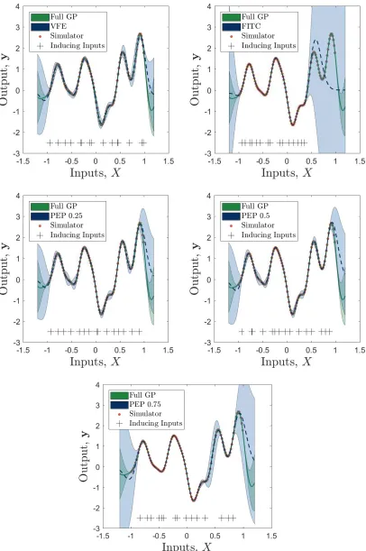
Fig. 3: Predictions from posterior approximation and FITC sparse GPs with 15 inducing points, against a full GP and training simulator data for a numerical example. Shaded regions indicate±3σ
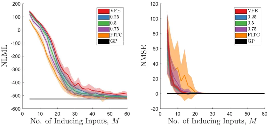
Fig. 4: The effect of the number of inducing inputsM andαon the performance of the PEP
formula-tion of sparse GPs averaged over 25 repeats for the negative log marginal likelihood (NLML, left) and the normalised mean squared error (NMSE, right). Shaded regions indicate±σconfidence intervals.
Figure 3 and Fig. 4 demonstrate the effect of additional inducing points and theαparameter for
a different one-dimensional numerical example. Here the simulator output is a sample from a GP (random seed integer of5is used in MATLAB) with zero mean and a squared exponential covariance function;σ2
f = 1, ψ = 30. Sparse GPs models were created withα = 0, 0.25, 0.5,0.75, 1and are
compared to the full GP solution and training data in Fig. 3, where mean and±3σconfidence intervals
are presented. A stochastic optimisation method was utilised for inferring the hyperparameters with 25 repeats to quantify the variance in the inference, presented in Fig. 4 as±σconfidence intervals. It
is demonstrated that the negative log marginal likelihoods (NLML) (−logp(y|X)) ≈ −Fv(Z) ≈ −logZP EP) reduce as more inducing points are added, stating that the model better explains the
data given more inducing inputs. The NLML also increases withα, in contrast, the normalised mean
squared error (NMSE) (Eqn. 15) is high with larger variance for FITC, a clear indication that the method has experienced overfitting. It is noted that there is significant overlap in NMSE results for VFE and PEP whenα= 0.25,0.5, indicating their predictions are very similar.
N M SE= 100
N σ2 y
∑
(f∗−y)2
(15)
Wheref∗ is the mean prediction of the GP emulator,yandσ2
y are a set of true simulator outputs
and their variance respectively. The NMSE formulation means that a score of zero indicates a mean prediction without error and a score of 100 for scenarios where the prediction is no better than taking the mean of the true values.
The PEP approach, whenα = 0.25, 0.5 provides better predictions of the data when compared to FITC and PEP atα = 0.75, demonstrated by low NLMLs that correspond to low NMSEs. FITC
and PEP when α = 0.75, although showing low NLMLs, have high NMSEs with large variance,
especially when the number of inducing points is low; which is a clear sign of overfitting. VFE tends to have high NLML with comparable NMSE to PEP whenα = 0.25,0.5. Figure 3 demonstrates that
the variance of the VFE prediction is larger than the full GP solution, with the variance of both the PEP formulations whenα = 0.25,0.5visually matching the full GP more closely. For these reasons it can be argued that PEP when α = 0.25,0.5preforms better in these examples. A close inspection of the NMSE in Fig. 4 for PEP when α = 0.5, demonstrates lower values than any of the posterior
values (FITC and VFE included) which is consistent with the findings of Bui et al [12]. The question still arises of how to choose theαparameter. Optimisation is not advised as a value of 1 will lead to
overfitting due to the FITC approximation. It is the experience of the authors that a value of0.5should give satisfactory performance, in-keeping with the finding of Bui et al. [12].
Considerations for Sparse GP Emulators. There are two main reasons why a sparse GP approx-imation can be useful in creating an emulator. Firstly, when a relatively large number of simulator runs are available, a sparse approximation can make inference practical. This is achieved by reducing the computational time complexity toO(N M2
)per simulator observation and reducing the memory requirement. Secondly, when predictions are required at a large number of test inputs a moderate com-putational saving is made,O(M)andO(M2
)per test point. Applications of when these reasons may be applicable is presented in this section.
In the authors opinion, it is not commonplace that the simulator is run at a large number of param-eter combinations. This problem mainly arises in a high dimensional paramparam-eter space where most of the parameters actively and significantly effect the output. Here even a space-filled design will result in a large number of simulator runs and a sparse GP approximation is applicable. Sparse GPs are more useful in a Bayesian optimisation [4, 5] or Bayesian history matching setting [6, 7]. Both methods often require predictions from the emulator for a large number of parameter combinations in order to accurately assess the output space for optimal solutions. The moderate computational saving in the prediction per test point means that a better exploration of the space can be performed. This becomes more important in a sequential design process for adding additional simulator runs to the optimisation, as used in an entropy search or information gain approach [4]. These methods often predict based on a set grid size for the parameter space; reducing the computational load for prediction means a finer grid can be set. Due to the approximate nature of sparse GPs their use is not always needed or favourable for creating emulators. The approximation introduces a nugget term that cannot be fixed as it is a cou-pling between a noise parameter for the data and an estimation of the error introduced by a low rank approximation. This means that deterministic predictions at know simulator outputs are not possible, as is the case with the full GP emulator. This has to be considered when the code uncertainty affects the results of additional processes, as is the case with Bayesian optimisation and Bayesian history matching.
Duffing Oscillator Case Study
A case study is presented showing emulation of a design parameter space for a duffing oscillator — defined in Eqn. 16 — as motivation for the use of sparse GPs as emulators within an early design context. The objective of this case study is to demonstrate the ability of a sparse GP, using the PEP formulation withα= 0.5(due to the reasoning from the previous section), to emulator a large design space based. Specificity, the aim is to emulate a5×5parameter grid of stiffnesskand cubic stiffness k3 terms that relate to a512point displacement time historyy— the total space being12800points.
In order to predict across this design parameter space an emulator is trained on a five simulator evalu-ations from a generalised Latin hypercube design where for each evaluation a512point displacement history is generated.
F =my¨+cy˙+ky+k3y 3
(16) The duffing oscillator in this case study has a mass ofm = 25kg and a damping ratio of ζ = 0.8with which the damping coefficient cis calculated. The forcing F is a 512 point random-phase multisine input [21] displayed in Fig. 5. The grid of stiffness and cubic stiffness coefficients used to test the performance of the emulator arek = {600,650, . . . ,800}N/m and k3 = {4×10
5
,5.25× 105
, . . . ,9×105
}N/m.
show-0 5 10 15 20 -800
[image:13.595.151.445.68.292.2]-600 -400 -200 0 200 400 600 800
Fig. 5: Random-phase multisine force input for the duffing oscillator.
ing an very good fit to the data. Due to the large space being predicted a zoomed in example of the prediction is presented in Fig. 6. The results show that sparse GPs can be used to capture large design parameter spaces, and therefore could be implemented inside an uncertainty quantification or design optimisation technique. The example also shows that the code uncertainty predicted by the emula-tor reflects both the sparse assumption and the size of the training set. In an optimisation context, if incorporated this uncertainty would ensure that parameter space is not excluded due to poor emulation.
Fig. 6: A zoomed in section of the sparse GP emulator (PEP withα = 0.5and250 inducing points) for the duffing oscillator displacement output across the5×5design parameter grid of stiffnesskand
[image:13.595.152.417.453.655.2]Conclusions and Further Work
GP emulators are powerful tools for exploring outputs from an expensive simulator. The approach can be especially useful in a Bayesian optimisation or Bayesian history matching settings. Here code uncertainty can be informative as to where to sequentially add the next simulator runs. The problem with GP models are that they are orderO(N3
)to train and are orderO(N)andO(N2
)for mean and variance predictions per test point. In settings where the simulator is very expensive and the design space is small a full GP solution is practical. However, some applications require a large number of simulator runs if the parameter space is high dimensional and necessitates a combinatorial approach to selecting inputs to understand the simulator output. In this scenario, sparse GP models are appropriate as they reduce the computational load of training toO(N M2
)where a prediction is of the orderO(M) andO(M2
)for the mean and variance respectively. Sparse GPs are also useful when a large number of predictions are required, as is the case in Bayesian optimisation and Bayesian history matching, where a moderate computational saving can be made.
There are two main approaches to sparse GPs, model or posterior approximation approaches. It has been demonstrated that model approximation methods will result in overfitting, due to the inducing points being parameters of a parametric model. For this reason, both a DTC and FITC approach are often not appropriate for sparse GP emulators. On the other hand, posterior approximations provide a solution by treating the inducing points as part of the inference, keeping the model exact and the method non-parametric. The two main approaches to posterior approximation methods are VFE and PEP. It has been shown that VFE will often smooth through the data, due to the trace penalisation term, resulting in predictions that overestimate the noise. PEP resolves these issues by reducing the penalty and generally outperforming VFE (especially whenα = 0.5). Therefore, it is recommended
that when sparse GPs are appropriate a PEP approximation should be used for generating emulators as this provides satisfactory performance.
Further research should be conducted into creating local approximations whilst retaining a global predictive quality. This could be achieved with a partially independent training conditional (PITC) approach where inducing parameters are fixed at known training points where the simulator output is of interest — for example where a maxima or minima is located. This would provide benefits in using the computational savings of a sparse approach will producing full GP inference around local regions of interest.
References
[1] Jerome Sacks, William J. Welch, Toby J. Mitchell, and Henry P. Wynn. Design and Analysis of Computer Experiments. Statistical Science, 4(4):409–423, 1989.
[2] Anthony O’Hagan. Bayesian analysis of computer code outputs: A tutorial. Reliability Engi-neering & System Safety, 91(10-11):1290–1300, oct 2006.
[3] Marc C. Kennedy and Anthony O’Hagan. Bayesian calibration of computer models. Journal of the Royal Statistical Society: Series B (Statistical Methodology), 63(3):425–464, 2001.
[4] Philipp Hennig and Christian J. Schuler. Entropy Search for Information-Efficient Global Opti-mization. Journal of Machine Learning Research, 13:1809–1837, dec 2012.
[5] Jasper Snoek, Hugo Larochelle, and Ryan P. Adams. Practical Bayesian Optimization of Ma-chine Learning Algorithms. InNIPS, pages 2951–2959, jun 2012.
[7] Paul Gardner, Charles Lord, and Robert J. Barthorpe. Bayesian History Matching for Forward Model-Driven Structural Health Monitoring. InProceedings of IMAC XXXVI, 2018.
[8] Anthony O’Hagan and John F. C. Kingman. Curve Fitting and Optimal Design for Prediction.
Journal of the Royal Statistical Society: Series B (Statistical Methodology) (Statistics in Society), 40(1):1–42, 1978.
[9] Carl E. Rasmussen and Christopher K. I. Williams. Gaussian processes for machine learning., volume 14. 2004.
[10] Joaquin Quiñonero-Candela and Carl Edward Rasmussen. A Unifying View of Sparse Approxi-mate Gaussian Process Regression. Journal of Machine Learning Research, 6:1939–1959, 2005. [11] Edward Snelson and Zoubin Ghahramani. Local and global sparse Gaussian process
approxi-mations. In11th International Conference on Artificial Intelligence and Statistics, 2007.
[12] Thang D. Bui, Josiah Yan, and Richard E. Turner. A Unifying Framework for Gaussian Pro-cess Pseudo-Point Approximations using Power Expectation Propagation. Journal of Machine Learning Research, 18(1):3649–3720, 2017.
[13] Edward Snelson and Zoubin Ghahramani. Sparse Gaussian Processes using Pseudo-inputs. In
NIPS, pages 1257–1264, 2005.
[14] Michalis Titsias. Variational Learning of Inducing Variables in Sparse Gaussian Processes. In
AISTATS, volume 5, pages 567–574, 2009.
[15] James Hensman, Nicolo Fusi, and Neil D. Lawrence. Gaussian Processes for Big Data. In
Twenty-Ninth Conference on Uncertainty in Artificial Intelligence (UAI2013), pages 282–290, sep 2013.
[16] Hildo Bijl, Jan Willem van Wingerden, Thomas B. Schön, and Michel Verhaegen. Online sparse Gaussian process regression using FITC and PITC approximations. IFAC, 48(28):703–708, 2015.
[17] Noel Cressie. Statistics for Spatial Data. Terra Nova, 4(5):613–617, 1992.
[18] Ioannis Andrianakis and Peter G Challenor. The effect of the nugget on Gaussian process em-ulators of computer models. Computational Statistics & Data Analysis, 56(12):4215–4228, dec 2012.
[19] Leonardo S. Bastos and Anthony O’Hagan. Diagnostics for Gaussian Process Emulators. Tech-nometrics, 51(4):425–438, 2009.
[20] Matthias Bauer, Mark van der Wilk, and Carl Edward Rasmussen. Understanding Probabilistic Sparse Gaussian Process Approximations. InNIPS, pages 1533–1541, 2016.
[21] Rik Pintelon and Johan Schoukens. System Identification: A Frequency Domain Approach.