The relevance of larval biology on spatiotemporal patterns of pathogen connectivity among open-marine salmon farms
Danielle Cantrell, Ramón Filgueira, Crawford W. Revie, Erin Rees, Raphael Vanderstichel, Ming Guo, Michael G.G. Foreman, Di Wan, Jon Grant
D. Cantrell: Department of Health Management, Atlantic Veterinary College, University of Prince Edward Island, 550 University Ave, Charlottetown, PE, Canada, C1A4P3.
Email: [email protected]
R. Filgueira: Marine Affairs Program, Dalhousie University, 6299 South St, Halifax, NS, Canada, B3H 4R2 Email: [email protected]
C.W. Revie: i) Department of Health Management, Atlantic Veterinary College, University of Prince Edward Island, 550 University Ave, Charlottetown, PE, Canada, C1AP3.
ii) Department of Computing and Information Sciences, University of Strathclyde, 26 Richmond Street, Glasgow, G1 1XQ, Scotland, UK
Email: [email protected]
E. Rees: i.) Department of Health Management, Atlantic Veterinary College, University of Prince Edward Island, 550 University Ave, Charlottetown, PE, Canada, C1AP3.
ii.) Land and Sea Systems Analysis, 14 rue Long, Granby, QC, Canada, J2G 6S8 Email: [email protected]
R. Vanderstichel: Department of Health Management, Atlantic Veterinary College, University of Prince Edward Island, 550 University Ave, Charlottetown, PE, Canada, C1A4P3.
Email: [email protected]
M. Guo: Institute of Ocean Sciences, Fisheries and Oceans Canada, 9860 W Saanich Rd, Sidney, BC, V8L5T5 Email: [email protected]
M.G.G. Foreman: Institute of Ocean Sciences, Fisheries and Oceans Canada, 9860 W Saanich Rd, Sidney, BC, V8L5T5 Email: [email protected]
D. Wan: Institute of Ocean Sciences, Fisheries and Oceans Canada, 9860 W Saanich Rd, Sidney, BC, V8L5T5 Email: [email protected]
J. Grant: Department of Oceanography, Dalhousie University, 6299 South St, Halifax, NS, Canada, B3H 4R2 Email: [email protected]
Corresponding author: Danielle Cantrell, Department of Health Management, Atlantic Veterinary College, University of Prince Edward Island, 550 University Ave, Charlottetown, PE, Canada, C1A4P3.
Abstract
Warming waters are changing marine pathogen dispersal patterns and infectivity worldwide.
Coupled biological-physical modelling has been used in many systems to determine the
connectivity of vulnerable meta-populations via infectious disease particles. Here we model the
connectivity of sea lice larvae (Lepeophtheirus salmonis) among salmon farms in the Broughton
Archipelago, British Columbia, Canada, using a coupled biological-physical model. The physical
model simulated pathogen dispersal, while the biological component influenced the survival and
developmental rates of the sea lice. Model results predicted high temporal variability in
connectivity strength among farms; an emergent effect from the interacting parts of the simulation
(dispersion vs. survival/development). Drivers of temporal variability were disentangled using
generalized additive modeling, which revealed the variability was most strongly impacted by the
spring freshet event, which can act as a natural aid for sea lice control in the Broughton
Archipelago. Our results suggest that farm management strategies can benefit by taking into
account short-term spikes in regional pathogen connectivity among farms. Additionally, future
scenarios of a warming climate with reduced snowpack will likely make sea lice control more
challenging.
Introduction
Transmission of water-borne pathogens (parasites, viruses, bacteria) in marine environments depends on factors influencing the movement and viability of the pathogen. Passive dispersal depends on local hydrodynamics, as dictated by winds, salinity gradients arising mainly from
freshwater discharges, air-sea heat exchanges, and/or tidal forcing (Foreman et al. 2009). Some
pathogens, particularly parasites with a free-living larval stage, possess some movement
round worms) have a free swimming larval stage and several intermediate hosts before ultimately
infecting marine mammals or, in some cases, humans (Lunneryd et al. 2015). Sea lice, an
ectoparasite of commercially and ecologically important fish species (Jones et al. 2006; Costello
2006), also possess a free-swimming larval stage, that influences their horizontal dispersal abilities
(North et al. 2008; Johnsen et al. 2016); however, they are still largely dependent on local
hydrodynamics for large scale (i.e. on the scale of kilometers) dispersal.
Additionally, the ability of water-borne pathogens to infect or infest a host can be influenced by the physical properties of the water they encounter, which can impact the growth, survival, and/or maturation of the pathogen (Brooker et al. 2018). For example, viruses will eventually degrade under ultraviolet B exposure (Jacquet and Bratbak 2003); bacterial or fungal pathogens can
become spores in unfavourable abiotic conditions, to become infectious later in conditions more
suited to their survival (Lennon and Jones 2011); temperature can impact bacterial replication rates
and temperature stress can make hosts more susceptible to bacterial infection (Holt et al. 1989),
and parasitic larvae development and survival rates are dependent on the water salinity and
temperature they encounter (Groner et al. 2016a; Samsing et al. 2016). In addition, in order for a
potential host to be vulnerable to contracting a water-borne pathogen, the host must come into
contact with a sufficient dose of viable pathogen (Schmid-Hempel and Frank 2007). However, the role that any of these processes involved in pathogen dispersion and viability may play in disease
transmission is difficult to determine.
Previous studies on water-borne disease transmission have frequently neglected important aspects related to the multifactorial nature of pathogen dispersion. For example, they often lack the
scale/epidemiological studies often use sea-way distance as a proxy for circulation (Aldrin et al. 2013; Rees et al. 2015). Studies that have explicitly modeled regional circulation (Stucchi et al. 2011; Adams et al. 2012; Asplin et al. 2014; Kough et al. 2015; Johnsen et al. 2016; Kragesteen et al. 2017; Salama et al. 2017; Samsing et al. 2017) typically do not elucidate the contributions of individual drivers to infectious pressure experienced by potential hosts.
The difficulty in determining epidemiologically important drivers of marine pathogen transmission
in real aquatic populations experimentally or observationally has led to the increasingly common
usage of computer simulations (Stucchi et al. 2011; Adams et al. 2012; Asplin et al. 2014; Kough
et al. 2015; Johnsen et al. 2016; Kragesteen et al. 2017; Salama et al. 2017; Samsing et al. 2017;
Arnold et al. 2017; Skarðhamar et al. 2018). These marine pathogen epidemiological simulations
often include: a physical circulation model, a simulated release of particles to be carried by/move
in the circulation (known as a particle tracking model), and a biological model of the lifecycle of
the disease assigned to the simulated particles. When all three models are simulated in sequence,
this can be referred to as coupled bio-physical modelling. Here, we apply a coupled bio-physical
model to the salmon farm, sea-lice system, with the ultimate aim of quantitatively determining which physical drivers lead to farms experiencing increased infective dose from their neighbouring farms.
Sea lice are a naturally occurring ectoparasite that affect salmon farming productivity and the health of wild salmonids (Revie et al. 2003; Jansen et al. 2012; Kristoffersen et al. 2014; Rees et al. 2015). In the northern hemisphere, Lepeophtheirus salmonis is the species of greatest concern
(Costello 2006), though other species, such as the more generalists Caligus clemensi can also
cause infestations. Sea lice attach to the scales of salmonids, and feed on the scales, mucus, and
behaviours (and thus growth), as well as make them susceptible to secondary infections (Mustafa et al. 2000; Wagner et al. 2008). In juvenile fish, infestations can result in death due to
osmoregulatory failure (Brauner et al. 2012; Patanasatienkul et al. 2013), though the levels
required to consider a juvenile to be ‘at risk’ have rarely been reported over the past decade (C.W.
Revie, pers comm). While the exact threshold size where juveniles are susceptible varies by species, generally they are most susceptible when smaller than 1 gram (Jones and Hargreaves 2009).
L. salmonis have several free-living larval stages after hatching, which can widely disperse, and
are usually located in the upper layer of the water column (less than five m of depth) (Johnsen et al.
2014). They do not become infectious and able to attach to a host until molting from nauplii into
copepods (Boxaspen 2006). The egg production, maturation rate, and survivorship of sea lice are
all dependent on the environmental conditions the louse encounters (Stucchi et al. 2011; Groner et
al. 2016a; Samsing et al. 2016). For example, warmer temperatures result in shorter maturation
time from larvae to maturity. Water below salinity thresholds results in death of the larvae or
reduced ability to settle on a host fish. What the threshold precisely is has not yet been agreed on
in the literature and likely varies between larval stages. However, Groner et al.’s 2016
meta-analysis on salinity’s impact on sea lice survival found a general trend of decreasing survival with
decreasing salinity, with 20 psu resulting in larval death (Groner et al. 2016a). The high fecundity
and wide larval dispersal capabilities of the sea lice life cycle benefit their overall survival and
success (Brooker et al. 2018).
A detailed understanding of sea lice dispersion and viability, and pathogens in general, should
salmon are subject to viruses, bacteria, and parasites requiring expensive treatments or large scale culls (Murray and Peeler 2005).Treatments have economic and environmental costs associated with their use to control disease outbreaks, and resistance to such treatments is a growing concern
worldwide for nearly all farmed salmon pathogens (Lees et al. 2008; Grøntvedt et al. 2014; Aaen
et al. 2015; McEwan et al. 2015). Farm-to-farm transmission of pathogens is common in some
areas, where connected clusters of farms must be treated together, or else re-infection is likely.
This has been most well studied in European farming areas (i.e. Scotland and Norway) (Adams et
al. 2012, 2015; Stene et al. 2014; Murray and Gubbins 2016; Samsing et al. 2017). Additionally,
there is concern over the potential for farms to amplify and introduce diseases at higher densities
to wild salmonid populations(Dill 2011; Kristoffersen et al. 2018; Nekouei et al. 2018).
Understanding connections among farms via pathogen transmission, and which environmental
factors contribute to periods of larger infective pressure can help industry coordinate regional
disease interventions as epidemiologically sensible management areas (e.g. groups of farms that
need to be treated as a single unit to minimize outbreak potential) (Aldrin et al. 2013; Adams et al.
2015; Samsing et al. 2017). Selecting the correct spatial and temporal resolution for management
of treatments, stocking/fallowing timing (Adams et al. 2016), and planning of future site locations
is crucial for continued aquaculture sustainability, for quality and quantity of animal production,
and for environmental sustainability to reduce the impact of pathogen spill-over to neighbouring
wild fish populations (Krkosek et al. 2013) .
the difference in the strength of the connectivity among farms via infectious sea lice larvae under
four different simulations, with increasing complexity in the biological model.
The population level patterns were then explored using generalized additive modelling (GAM) to
elucidate the drivers of temporal variability in the infective dose farms exert on each other. This
analysis also assessed whether drivers of temporal variability in the connectivity of farms varied
spatially.
Methods
Study site and simulation period
The model domain is the BA, BC, Canada (Fig. 1); a group of islands off the northeastern tip of
Vancouver Island. It is the site of a currently active salmon farming industry, as well as an
important part of juvenile wild salmonid migratory routes for Pink (O. gorbuscha), Coho (O.
kisutch), and Chum salmon (O. keta), and to a much lesser extent, Sockeye (Oncorhynchus nerka)
and Chinook (O. tshawytscha). It is a highly complex and fjordic area, with currents driven by
tides, winds, and freshwater runoff from rivers whose discharges generally peak in the spring
(Foreman et al. 2015) . Channels are as deep as 600 m, though most range between 50-300 m
(Foreman et al. 2006), and sea surface temperatures have a narrow range, from an average of 7.1C
in January to 10.9 in August (Rogers et al. 2013).
The underlying physical model was constructed using the Finite Volume Community Ocean
March 11th, and ran to July 31st, 2009. The March-July time frame was chosen because this is the period during which the wild juvenile salmon will typically out-migrate from the rivers in which
they were spawned to the open ocean.
The bio-physical model
The underlying circulation model is an update of that described in Foreman et al. (2009) to include
air-sea heat exchanges. These exchanges have four components: sensible heat flux (differences in
temperature between the air and water), latent heat flux (heat arising in changes between states,
such as evaporation), short wave radiations (e.g. solar, some of which may be absorbed by clouds
as well as ground and water), and long wave radiation (i.e. energy that the ground and water
re-emit back to the air).
The model domain is shown in Foreman et al. 2009, Fig. 1. There were 21 vertical gridded layers with variable spacing from sea bottom to surface, with the highest resolution at the surface and bottom layers, and maximum inter layer spacing of 9% of the depth at mid column. Depth ranged
between 3 m and 520 m (Cantrell et al. 2018). Daily freshwater river discharge values were used
(see Fig. 1 for river locations). M2, N2, S2, K1, P1, and O1 tidal constituents were prescribed as
forcing at the model boundaries, and hourly tidal data was used. Hourly wind forcing data was
captured with 9 weather stations deployed across the BA, with winds interpolated between and
extrapolated beyond station locations to all grid elements (Foreman et al. 2009). The FVCOM
physical circulation model outputs (i.e. wind, temperature, and salinity fields, and resulting
currents) were validated by comparing model and observed tidal harmonics and calculating
correlation coefficients between observed and modeled currents at several different depths at five
good agreement, with the correlation coefficient worst at 4.5 m (0.74), and improving with depth,
to a correlation coefficient of 0.94 at 130 m depth (Foreman et al. 2009).
Hourly output from the hydrodynamic model was used by an offline particle-tracking model, in
which each simulated particle represented a cohort of sea lice larvae. Each of these particles was
coupled to a biological model that dictated the maturation and survivorship of the particle based on
the salinity and temperature it encountered(Stucchi et al. 2011; Cantrell et al. 2018).
The details of the equations governing the biology of the sea lice larvae can be found in (Cantrell
et al. 2018). In short, particles where released as pre-infectious nauplii, which matured into
infectious copepods at a rate that was temperature dependent. The relationship between
temperature and maturity was set as a Bělehrádek equation, with lower temperatures resulting in slower maturation rates Additionally, salinity impacts nauplii particle survival, with salinity below
30 psu resulting in decreased survival. Survival decreased at a constant rate once particles matured
into copepods due to a lack of agreement in the literature as to the precise relationship between
salinity and survival for sea lice copepods.
The offline particle-tracking model simulated the release of 50 particles from each farm (n=20)
every hour, for the duration of the simulation. Each release of particles is referred to as a pulse.
The first day of pulses began on March 11th, 2009, and the last day of pulses was on July 20th, resulting in 129 total days, and 3096 pulses. The location and status of each particle was tracked
for 11 days, in order to simulate the hypothetical lifespan of a sea lice copepod in the temperature
Connectivity calculations
Details of the methods used to calculate connectivity using the particle tracking releases can be
found in Cantrell et al. (2018). In brief, the infestation pressure (IP) each farm exerted on every
other farm was estimated as follows: a cohort of sea lice was defined as 24 hours of particle pulses,
and each of these groups was labelled as a “cohort release day” (CRD). The offline
particle-tracking model recorded location, maturation, and survivorship of all particles in each CRD every
24 hours for 11 days. These 11 “snapshots” taken for 24 hours worth of pulses were then
combinedinto a single shape file. Thus, each CRD represents the entire life of a cohort of particles
released from all farms on one particular day of the simulation (Fig. 2 in Cantrell et al. 2018).
Each CRD was then separated by emitting farm (i.e. all particles released from a single farm) and
used as the input for kernel density estimations (KDE), which were then saved as raster files (129
CRDs x 20 farms = 2,580 raster files). From each raster file, the density of particles at the grid
section in which each farm was located was extracted. This density represents the IP that a given
farm exerted on all other farms as well as on itself (self infestation), measured in particles km-2. These densities were stored in connectivity matrices, which were then summed and averaged
(mean) for all 20 farms per CRD. These matrices could then be used to estimate a mean
connectivity value for all connections in the entire network of farms for each CRD in the
simulation. Using this methodological approach, Cantrell et al. (2018) identified four distinct
Farm connectivity with different biological drivers (i.e. maturation and survivorship)
The mean connectivity score for every CRD was calculated for the entire network and for the four
sub-networks. Additionally, each sub-network’s mean connectivity was calculated under four
different scenarios to determine the relative contribution of the maturation and survivorship
coefficients of the biological model by investigating the differences between the following four
simulation scenarios:
I. Physical simulation only, which excludes all parts of the biological model (particles
are passive);
II. Physical simulation plus survivorship simulation, which excludes the impacts of
temperature (includes only the impact of salinity on the survivorship in the biological
model and the physical simulation);
III. Physical simulation plus maturation simulation, which excludes the impacts of
salinity on the biological model (includes only the impacts of temperature on the
maturation in the biological model, and the physical simulation);
IV. Physical simulation plus maturation and survivorship simulation, (includes the impact from both temperature and salinity on the maturation and survivorship,
respectively, and the physical simulation).
Generalized Additive Model to determine drivers of connectivity strength
A GAM approach was used to identify environmental and biological factors influencing the
emergent pattern seen in temporal variability in network connectivity. This modelling approach
was chosen because GAM allows the relaxing of the assumption of linearity between the predictor
and response variables by combining spline functions into a smoother line that best describes the
relationship. GAMs also do not need to determine the functional form of the relationship
beforehand (Guisan et al. 2016). Each sub-network was modelled separately in order to account
for the hierarchy in the data and facilitate interpretation of the results, rather than using a
generalized additive mixed model (GAMM). The response variable was the mean connectivity per
CRD for the sub-network. Four independent predictors were assessed:
I. River discharge in m3s-1, as measured at river mouths in the BA (discharge contributions from eight rivers, with each river assigned to the closest sub-network);
II. Daily solar heat flux value in watts m-2 (identical across the model domain);
III. Either maximum daily or mean daily “along channel” wind velocity in ms-1, extracted from a location near each sub-network, which ever was more significant (coordinates in the
supplementary materials). The sign of the wind gust (i.e. positive or negative) indicated
wind direction (i.e. “up channel”, or seaward). The cross channel wind direction was not
used, as it is unlikely to contribute significantly to the movement of particles up or down
the channels. The maximum daily wind velocity was the more significant predictor for
networks 1, 2, and 4. Mean wind velocity was the more significant predictor for
sub-network 3;
IV. Daily tidal range (maximum minus minimum sea surface height) in m, from the Port Hardy
surface height values have the potential to be impacted by other factors, such as winds.
However, in this case, there was no collinearity observed between tidal height and other
predictors, and tides are the main drivers of sea surface height in this area.
Given that each CRD includes 11 days worth of connectivity information, each predictor was
calculated as a rolling 11-day average to mirror the CRD structure. This resulted in a time series of
129 time points, each an 11-day rolling average.
Each independent predictor was used as an individual predictor first. Any sub-networks that had
more than one predictor with a p-value < 0.15 were then modelled with all possible combinations
of these predictors, including interactions. The top model was selected using AIC model selection
techniques to maximise explanatory power with model parsimony (Burnham and Anderson 2002).
The time series of all predictors (river discharge, heat flux forcing, winds, and tides) were checked
for autocorrelation using an autocorrelation function (“acf” command in the mgcv package in R)
(Wood 2006), (R core team, 2018). All predictors showed substantial autocorrelation, so an
auto-regressive term was included in all models. The value of rho for each model was computed by
extracting the lag 1 value from the autocorrelation function residuals of each model. Rho values
ranged from 0.77-0.9. The fast restricted maximum likelihood method was used for model
building and comparisons (command, method =“fREML” in the bam() command of the mgcv
package in R) (Wood 2006). The number of knots for all models was set using generalized cross
validation in the mgcv package in R (Wood 2006). Heat flux and river discharge demonstrated
collinearity (possibly because hotter days could result in more run-off from snow melt, though
added to each plot of predictor vs. sub-network in order to more easily visualize the relationship
between the two.
Sensitivity Analysis
A sensitivity analysis of the biological parameters (maturation and survivorship) was conducted
for sub-network 2 (farms 6-7, and 16-18), because this sub-network most closely reflected the
overall trend seen when all farms were grouped together (i.e. sub-network 2 also showed evidence
of the four peaks seen in the overall connectivity plot, at the beginning of the simulation and at
CRDs 59, 93, and 123, as seen in Fig. 2D). The sensitivity tests consisted of four simulations,
where the values for maturation or survivorship for each particle for each time step was adjusted in
the following ways: maturation decreased to 50%; maturation increased to 150%; survivorship
decreased to 50%; survivorship increased to 150%.
The total IP that the farms in sub-network 2 exerted on all of the other farms was calculated for
every CRD in the simulation. Self-infestation was excluded to highlight the strength of
connectivity among farms (i.e. the likelihood of parasite transmission between farms), rather than
emphasizing CRDs that had high connectivity within farms. This IP was plotted for every CRD,
and the results of the four simulations were compared with the simulation based on the full
biological model (with both survivorship/maturation at their default levels).
Results
Overall farm connectivity strength under different scenarios
The strength of the network connectivity for the physical model simulation is the highest of the
simulation (Fig. 2a) also has less temporal variability than the other simulations. The IP
experienced per CRD ranges roughly between 7.8 and 10 particles km-2, representing 22% variation.
The survivorship only simulation (Fig. 2b) had lower connectivity strength than the maturation
only simulation (Fig. 2c). The IP ranged between roughly 0.6 and 2.4 particles km-2, representing 75% variation. The survivorship only simulation also had a peak at the start of the simulation,
followed by a gradual decrease for the remainder of the simulation. There are no peaks at CRDs 59,
93 and 123, as seen in the survivorship/maturation simulation (Fig. 2b) or the maturation
simulation (Fig. 2c).
Not surprisingly, both simulations with only a portion of the biological model (the maturation only
and survivorship only simulations) showed connectivity strength and variability intermediate
between the physical model and full biological model (survivorship/maturation) simulations. The
IP in the maturation only simulation (Fig. 2c) ranged from roughly 3.5 to 7.5 particles km-2, representing 53% variation. This simulation has a similar pattern to the full biological model
simulation (Fig. 2d) in that there is a peak in connectivity in the beginning of the simulation that
decreases over the first 20 CRDs, though the peak is smaller than that seen in the
maturation-survivorship simulations. The peaks in connectivity at CRD 59, 93, and 123 also exist in the
maturation simulation.
The survivorship-maturation simulation has the lowest overall connectivity (Fig. 2d), decreased by
an order of magnitude over the purely physical simulation. The infestation pressure ranges roughly
emerges, with the initial CRDs having a much higher overall connectivity than the rest of the
simulation, and then sharply decreasing over the first 20 CRDs. There are also distinct peaks
around CRDs 59 and 93, and a smaller peak around CRD 123. Possible reasons for this pattern are
explained in the discussion.
Sub-network connectivity differences
The drivers of the temporal variability were also explored by sub-network for the simulation that
included all aspects of the biological model (the survivorship/maturation simulation). Sub-network
1 (Fig. 3a) and sub-network 4 (Fig 3d) do not have peaks at CRD 123. Additionally, the initial
peak in connectivity strength is lower than in sub-networks 2 or 3. Sub-network 2 (Fig. 3b) has
the same steep starting peak, as well as peaks at CRD 59, 93, and 123 that are present in Fig. 2d.
Sub-network 3 (Fig. 3c) has only a small increase at CRD 59. Sub-network 4 (Fig. 3d) has a low
overall connectivity. However, even with the low connectivity, there is still a slightly higher
connectivity at the start of the simulation, as well as at CRD 93.
The maturation only simulation resulted in a 40-68% reduction in the AUC depending on network.
For the survivorship only simulation the reduction in AUC was greater than 80% for all
sub-networks. When the full biological model (survivorship and maturation) was used the value of the
AUC was reduced by over 99%.
Salinity and temperature as drivers of the biological model
The mean salinity that each cohort encountered over the 11-day tracking period suggests that there
was an overall decrease in salinity throughout the entire simulation period (Fig. 5a) coinciding
not monotonic here). The temperature drops during the first 20 or so CRDs, but with a subsequent
upswing peaking at CRD 59. There is a second increasing trend with a peak at CRD 93, with the
temperature remaining higher until the end of the simulation, and a small peak again at CRD 123
(Fig. 4b). The water temperature increased on these days due to increases in the heat flux (Fig. 5b).
Within each individual cohort, there is a hooked shape seen in both Figs 5a and 5b. Cohorts start
out at a lower salinity (Fig. 5a) and higher temperature (Fig. 5b). Salinity increases and
temperature decreases over the CRD life, and then levels out slightly lower than the maximum
salinity, and slightly higher than the minimum temperature. This shape is due to the vertical
velocity components. Because the particles have not been assigned either a swimming ability to
combat these downward velocities or a density that would stop descent when neutral buoyancy
was attained, they moved passively with the downward (on average) vertical currents from the
near-surface depths where they were released (until reaching the maximum depth constraint of
5m).
Additionally, Figs. 5a and 5b have a secondary axis, showing the instantaneous survivorship and
maturation for each day of the simulation with that daily temperature and salinity input into the
equations governing maturation and survivorship. The secondary axis shows the close relationship
between the temperature and salinity experienced by particles and the instantaneous maturation
and survivorship of the particles, with each increasing or decreasing together. The threshold in the
survivorship equation is apparent in approximately the first 45 CRDs in Fig 5a, where survivorship
Drivers of connectivity strength
The independent predictors included in the GAM model were the 11-day rolling averages of the
daily values of river discharge, total heat flux forcing, wind, and tidal range (Fig. 4). The same
plots for the river discharge and winds, but showing individual river discharge and weather station
wind gusts, respectively, are in the supplementary materials.
The relationship between all predictors and the connectivity for each sub-network has been
graphed with smoothed plots in Fig. 6. Thus, the impact of river discharge on connectivity is
roughly a nonlinear, negative relationship. When the river discharge increases, connectivity
decreases as water with lower salinity floods the system. Thus, river discharge is a proxy for
salinity (and thus lowers survivorship of sea lice particles). Sub-networks 1-3 were dominated by
the river discharge (Fig. 6a-d), with between 56-74% deviance explained by river discharge alone.
Total heat flux forcing (Fig. 6e-h) has the opposite, also nonlinear relationship, with increasing
connectivity as temperature increases. Heat flux was significant for all sub-networks except 3.
Wind has a direction associated with the sign of the predictor, with negative indicating seaward,
and positive indicating “up channel” wind direction. Sub-networks 2 and 4 were significantly
predicted by wind, with the negative wind direction (seaward) having higher connectivity results
for both. Wind explained 42.9% deviance for sub-network 2 (Fig. 6j) and 13.6% of the deviance
for sub-network 4 (Fig. 6k). Despite this rather low deviance for sub-network 4, wind has the
largest explanatory power as a univariate predictor for this sub-network; the connectivity was not
Tidal range was only significant for sub-network 2 (Fig. 6m-g). The relationship is roughly linear
and negative, so as tidal range increases, connectivity decreases.
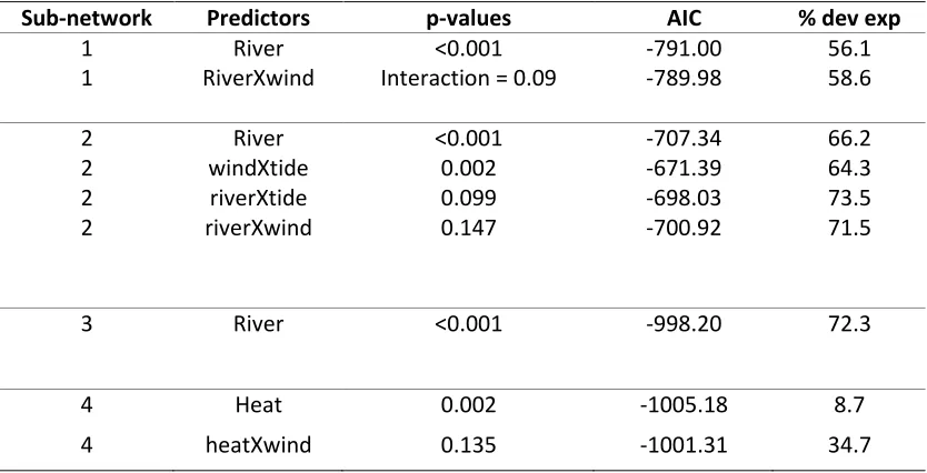
For all sub-networks, all predictors with p-values < 0.15 were combined, as well as their
interactions were tested in further GAMs (Table 3). The model for sub-network 1 did not improve
from adding additional predictors to the river discharge predictor alone, or have any significant
interactions. The top model based on AIC selection techniques from sub-network 2 was also from
river discharge as a predictor alone. However, the interaction for wind and tide was significant
(p=0.002), and the model with river discharge and the interaction between wind and tide
accounted for 82.3% of the deviance (despite having a higher AIC score). Sub-network 3 had only
one predictor (river discharge) as statistically significant, so no further predictors were considered.
The top AIC selected model for sub-network 4 included both heat-flux and wind, which resulted in
a still poor percent deviance explained, of 32.4%.
2009 as a representative year
To determine how representative the simulation period was (March-July, 2009), the main driver of
connectivity strength (river discharge) was plotted against a historical dataset of river discharge.
This historical dataset has 41 years of data on river discharge from the Kliniklani River (Fig. 7).
Kliniklani discharge data began to be collected in 1968, and continues currently, however we only
examined data up until the simulations time period (2009). The Kliniklani has the largest discharge
in the BA, and is thus the most important in terms of impact on local circulation (Foreman et al.
2015). The daily means for 2009 had 26 days during the simulation period that were outside of the
standard deviation for the 41-year daily means. These occurred around simulation day 50, 100, and
2009 was within the standard deviations of the 41-year average for the entire simulation period
(Fig. 7b). Thus, the two plots show that while there are a few days with variability outside of the
standard deviation of the 41 year mean, over all, 2009 remains well within what is “typical” for the
BA.
Sensitivity Analysis
Sensitivity analysis revealed that changing the maturation and survivorship parameters changed
the magnitude of connectivity, but not the pattern in the timing of temporal spikes (i.e. there are
still peaks on the same CRDs). The AUC calculations quantify the change in magnitude compared
to the full biological model (survivorship/ maturation) simulation (Table 2). The percent change
ranges from 38% to 414%, and changes in the maturation impact the AUC more than changes in
the survival. Fig. 8 is the mean connectivity for each CRD for the sensitivity analysis simulations.
Discussion
This study presents the output of a coupled bio-physical model of sea lice dispersal from salmon
farms in the BA. The results provide a framework for how to analyse output from such models to
quantify which processes affect the dispersion and viability of water-borne pathogens. The
connectivity of the farms displayed high temporal variability, an emergent pattern that results from
the many interacting aspects of both the biological and the physical model. GAM was used to
elucidate the main drivers of the population level behaviour in the simulation. These outputs
suggested that temporal patterns were largely dictated by the influence of the spring freshet, which
caused declines in the salinity and temperature of surface waters, and thus modulated the number
of particles that survived and matured into infectious copepodids. Thus, the temporal variability
with each particle in the simulation being impacted by the physical model conditions. The spring
freshet decreases survivorship and slows maturation for larvae located in the upper layers of water.
However, temporary spikes in connectivity can occur when temporary heat flux forcing spikes
lead to temperature increases into the ideal range for sea lice larval maturation (100% hatching and
development success was found to occur between 15-20 °Cby Samsing et al. 2016). Additionally,
spikes occurred when winds were blowing seaward, which allows particles to come into contact
with other farms, rather than being blown towards the top of the fjordic channels where it cannot
encounter another farm.
Temporal variability in pathogen viability
The rapid decrease seen in the first 20 CRDs of the survivorship/maturation simulation appears to
some extent in both the survivorship simulation, and the maturation simulation. Neither part of the
biological model clearly explains the entirety of the peak seen in the first 20 CRDs, suggesting the
impacts of the maturation and survivorship aspects of the simulation are cumulative.
An important part of the circulation of the BA is the spring freshet, when the snow in the
surrounding mountains melts. This results in fresh, cold water entering the BA through river
discharge at an average daily discharge rate upwards of 700m3s-1 by July. This was explicitly modelled in the underlying circulation model, and seems to be the single largest driving factor of
the changes in salinity that impact survivorship in the biological model. Salinity gradually
decreases as the simulation progresses (Fig. 5), with certain cohorts (i.e. around cohorts 105 and
135) experiencing even larger decreases in salinity. The decrease in salinity corresponds to a
decrease in survivorship. Additionally, temperature also drops during this time, also due to the
particles reaching maturation. Thus the first steep drop in connectivity seen in the full biological
model (the survivorship-maturation simulation) is due to the cumulative effects from a decrease in
salinity and temperature, driven by the spring freshet ramping up. This results in fewer infectious
sea lice copepods being present in the model domain, leading to a decrease in the strength of
connectivity across the entire network. The high impact of the spring freshet was confirmed by
GAM modelling, where between 56-76% of the deviance was explained by river discharge alone,
for sub-networks 1-3. The fact river discharge was so much more important as a predictor for
connectivity than heat flux forcing also confirms the importance of survivorship on connectivity,
which is driven by salinity.
The spring freshet might be acting as a “natural control” in the BA, slowing sea lice larval
development and thus helping to keep sea lice loads low, which has also been suggested elsewhere
(Brooks 2005). Thus with the current climate warming, a reduction in snowpack and glaciers is
expected to reduce this “natural control” effect (Kang et al. 2016; Najafi et al. 2017). Additionally,
warmer waters would result in shorter maturation times, and thus a higher density of infectious sea
lice larvae in the water column. This suggests sea lice infection pressure will increase with time if
climate change continues unabated (Bateman et al. 2016).
Despite the importance of the freshet event and salinity on overall farm-to-farm connectivity in sea
lice infection, we still find evidence for the importance of temperature on the temporal variability
of these connectivity patterns. In the BA, temperature can be regulated by the spring freshet (as
described above) and the heat flux forcing of the system to modulate surface water temperature.
We observe a decrease in temperature seen in the first 20 CRDs (due to the river discharge)
temporary increases in the heat flux forcing). These spikes appear in the simulation with both the
survivorship/maturation, and also appear in the maturation simulation, but not the survivorship
simulation. This demonstrates that maturation, which is dictated by temperature (which is in turn,
impacted by both the heat flux and the river discharge), is the main driver of the spikes in the
network strength on those particular CRDs. However, the spikes at CRDs 59, 93, and 123, do not
reach the connectivity strength seen at the start of the simulation (Fig. 2b). Thus, the heat flux
forcing alone was not enough to overcome the impacts of the river discharge on survivorship,
probably because of the countering effect of cold river discharge from snow and glacial run-off.
Additionally, the relatively colder, fresher water tends to stay mostly in a less dense upper layer in
the water column during a freshet event (particularly in fjordic areas), where sea lice are generally
located (Oppedal et al. 2017).
Temporal variability in disease connectivity has been observed in multiyear and annual
simulations from other regions. Samsing et al. (2017) ran bio-physical simulations of the
Norwegian west coast for six years and found strong seasonality in the farm-to-farm connectivity
of sea lice infection, with consistency of seasons across years; although connectivity drivers across
seasons were not discussed. Adams et al. (2016) simulated the Scottish west coast for one year,
and found farm-to-farm sea lice infection connectivity varied over time by a factor of two;
similarly, particular drivers of why this variation exists were not in the scope of the paper. This
suggests that high temporal variability in network connectivity strength in pathogen dispersal may
be the rule, rather than an exception, and thus any connectivity or larval dispersal simulations
could benefit from analyzing temporal variability. Additionally, any management
recommendations made from simulations should use a precautionary management approach, with
as even temporally short “pulses” of high connectivity strength can result in outbreak scenarios
(Velentgas et al. 2013).
Simulation time period
Our model simulates circulation conditions from March—July 2009. The representativeness of a
“typical” year for the BA is important for applying results to other years. Cumulative discharge for
2009 was within the standard deviation of the 41-year mean for the entire simulation period.
However, 17% of the days in the simulation period had daily discharge values outside of the
standard deviations of the 41-year daily mean, generally due to unusually large storm events, of
which there were none during our simulation period. River discharge was the most important
factor impacting connectivity across every connected sub-network of farms. (ie sub-networks 1-3).
Therefore, the circulation conditions of 2009 are likely relatively “typical” for the region, which
increases confidence in applying model results to other “typical” years. However, caution should
be used when applying results to non-typical years (i.e. years with unusually small snow pack in
the mountains and thus a smaller freshet event, or unusually warm years, or years when the freshet
timing may be off). These scenarios may be particularly important in the context of climate change.
Spatial drivers of pathogen dispersion
The fact that the four sub-networks resulted in different variables for creating the top selected
GAM models demonstrates that environmental drivers of connectivity can vary, even on relatively
small spatial scales. It is perhaps not surprising that the farms belonging to sub-network 4 were not
as impacted by river discharge as the other networks, given that the farms involved in this
sub-network are closer to the open ocean, and furthest away from the mouths of rivers compared to the
of discussion, they are in fact a group of independent, unconnected farms. Most of the particles
released from these farms were simply flushed out to sea. Thus, it is likely the connectivity was so
low for this sub-network, finding significant associations with any driver would be difficult, and
the top selected model of both wind and heat-flux only explaining 32.4% of the deviance is
perhaps to be expected. Likewise, the relationship of sub-networks 1-3 to river discharge is
perhaps not surprising, given the much closer proximity of these sub-networks to large river
mouths.
The GAM models indicate wind to be an important driver in sub-networks 2 and 4. Sub-network 2
is in a more closed, protected area of the BA. The negative wind direction (seaward) has a strongly
positive association with connectivity strength. This could be because wind in the seaward
direction (i.e. a south—westerly wind for sub-networks 1 and 2) would create surface currents that
would carry particles from these networks of farms into contact with other farms. For
sub-network 2, a southwesterly wind would push the particles towards each other, to circulate in the
area, rather than being flushed out and away from the farms. There is a less strong, but still
significant relationship between wind and connectivity strength in network 4. For this
sub-network, a north-westerly wind would push particles from farms 19-20 towards farms 8, 9 and
12-14, thus increasing connectivity amongst this low connected sub-network, rather than just being
flushed out of the BA before encountering other farms. Sub-network 1 was not significantly driven
by wind; however, this variable was retained in the top selected model. Furthermore, this
sub-network shares the same trend in wind direction (i.e. seaward resulting in the highest connectivity)
as observed for sub-networks 1 and 4. Only sub-network 3 did not share this trend and seemed to
such a large impact from the river discharge, it essentially “drowned” out any signal from other
drivers.
Tidal range was not detected by the GAM modeling approach to be an important driver in
farm-to-farm connectivity of sea lice infection. However, this could be due in part to the way the particles
were grouped in our analysis. Twenty-four hours of particle pulses where grouped together as one
“cohort”, which could alias the influence of tidal cycles. However, the 24-hour grouping of
cohorts would not mask tidal fluctuations longer than 24 hours in duration (e.g., spring and neap
tides), or seasonal variations in tides, such as the higher tides seen near the summer solstice. This
seasonal variation is more important from an epidemiological perspective, as individual tidal cycle
impacts would be for short period (on the scale of hours) and would essentially repeat daily. Thus,
the variation in IP strength caused from daily tidal cycles would be similar from day to day.
Additionally, the AUC calculations (Table 2) suggest that adding the survivorship of the particles
to the simulation results in a larger reduction in connectivity of the sub-networks. Survivorship
reflects mainly the impact of the freshet. The reduction in AUC from maturation (reflecting the
impact of both heat flux and the spring freshet) is both smaller and more variable across
sub-networks. This variation is likely a reflection of differences in time particles emitted from each
sub-network have around other farms before being flushed out of the vicinity. Sub-network 4 has
the largest impact from maturity, because it had very few particles connect with other farms. Thus,
adding the maturation restriction (i.e. the particles do not “count” in the first few days of their lives
as they are not yet viable) has a larger impact on this sub-network’s connectivity to the other farms
than the other sub-networks. Sub-network 2 has the lowest impact from maturity, as the time those
particles spend around other farms in the BA is quite high, thus adding maturity to the simulation
Impacts of changes in the biological model on connectivity strength
The sensitivity analysis revealed that changing the biological model outcomes by increasing or
decreasing the survivorship and maturation values assigned to each particle resulted in changes in
the strength of connectivity, but did not change the overall pattern observed. In other words, the
particles km-2 might increase with increasing maturation values, but the peaks seen at the beginning of the simulation, as well as at CRDs 59, 93, and 123 remained. This could be
important if the objective is to estimate exact infestation pressures, to keep exposure below a
certain infectious dose. However, in the case of sea lice, the infectious dose necessary to result in a
sea lice infestation is not known. Therefore, translating the absolute number of particles km-2 into absolute risk values is not yet possible (Frenzl 2014). It is, however, possible to consider relative
risk and recommend spatial management solutions that may reduce the likelihood of outbreaks.
These do not change whether the connectivity strength is small or large or orders of magnitude
different. Therefore, in the case of this particular study, the sensitivity analysis revealed that the
parameters are robust when the goal is to identify connectivity patterns.
Applied results for the salmon industry
Outputs from bio-physical simulations for disease management in aquaculture (not only for sea
lice, but for any larval and/or pathogen connectivity study) need to be validated by field data
before being implemented, as excluding key parts of larval biology can change the spatial
connectivity pattern and/or temporal variability tied to the life history of the larvae. Validation of
parasitic larvae dispersal models is difficult and expensive. Some attempts at validation with field
data include plankton tows in areas with higher risk of infestation pressure, as well as sentinel
the water column, typically fewer than five sea lice larvae are found in each standard tow. The low
sample size makes this method a less than ideal validation method. Additionally, it is difficult to
account for the impact of wild salmon on disease transmission, as wild salmon routes are not fully
known and sea lice connectivity simulations thus far do not explicitly model wild salmon
populations. Nevertheless, validation of this model must be undertaken before management
suggestions are implemented, and thus is the focus of ongoing research.
At this stage, the model output can allow for some practical recommendations for the salmon
farming industry in the BA. Model output suggests that outbreak scenarios are more likely to
result when river discharge is low. Years with less snow pack in the surrounding mountains could
contribute to more difficult sea lice management. Managers can also anticipate outbreaks during
warmer time periods, and during periods with seaward winds for each sub-network, which will
keep particles in the BA for longer, and thus result in a higher infestation pressure. This result is a
particular concern as the temperature of the BA coastal waters rise with global warming (Wolff et
al. 2017).
Additionally, the model could be used to simulate hypothetical scenarios to explore the
impact of management practices on sea lice transmission. For example, the effect of
coordinated treatment could be explored by analyzing connectivity after the removal of sea
lice from one/several farms at a given time
Any farms kept in current locations or future farms placed near current farm locations should
consider using these sub-networks as treatment areas for sea lice management, as treating only one
sub-network 4 could result in farms less connected via shared pathogens. Care should be taken to
not place farms near the current farm 11, which acts as a pathway to connect sub-networks 1 and 3
(see Cantrell et al. 2018). Model results suggest that farms located closer to the open ocean are less
likely to infect one-another; however, the role of farms in these locations to infect wild salmon
populations is not known and requires further investigation.
The relevance of sea lice biology on connectivity
Our simulations suggested that connectivity output from coupled bio-physical models is
potentially highly dependent on the biological model of the particle whose dispersal is being
simulated (in our case, the sea lice copepod). However, as recently highlighted in the review paper
by Brooker et al. (2018), there is no final consensus around the parameters or equations governing
sea lice biology. Thus, marine epidemiology, sea lice modelling, and spatial ecology scientific
communities would benefit from a consensus being reached on the impact of salinity and
temperature on the life history of the sea lice larvae.
There are conflicting reports on how salinity and temperature impact sea lice. For example, Groner
et al. (2015) used existing literature on salinity impacts on different life stages of sea lice to fit
salinity dependent logistic-mortality curves, and found that salinity has a non-linear effect on sea
louse survival, with most effects at less than 20 psu; a value substantially lower than the threshold
in our study, which was 30 psu. However, other studies found impacts of salinity on mortality
began at much higher salinity. For example, Bricknell et al. (2006) found that at 29 ppt survival
was severely reduced, and larvae had a reduced ability to sense or respond to the presence of a
reduced activity and survival below 25 ppt (Note that these studies measured salinity in different
units, ppt vs psu, but for practical purposes they are nearly equivalent).
In terms of impact of temperature on development time from nauplius to infectious copepod,
Gravil (1996), Boxaspen and Naess (2000), and Samsing et al. (2016) found different development
times based on nauplius stage, as well as impacts on egg development time. None of these
individual stages were explicitly modelled in our simulation, where particles were considered only
pre-infectious or infectious (i.e. copepodids). While lacking agreement on specific times for each
development stage, all studies on the impacts of temperature on maturation found a substantial
positive relationship, with warmer waters decreasing development time. This relationship suggests
that future scenarios of warming oceans could render control of sea lice more difficult (Groner et
al. 2014; Gallana et al. 2016; Cunningham et al. 2017; Algeo et al. 2019).
Model limitations
Our simulation did not explicitly model several aspects of sea lice larval life history. For example,
the impacts of salinity and temperature on egg hatching rates and success were not modelled.
Additionally, diel vertical migrations have been shown to impact horizontal dispersion of sea lice,
reducing dispersal lengths (Johnsen et al. 2016). Particles in our simulation were not given diel
migration behaviours, thus our simulation may over estimate dispersion lengths, which could
result in the sub-networks being identified to include farms that should not be included.
Settlement of infectious particles on hosts was also not explicitly simulated, though contact time of
infectious copepods and competition for space on hosts is known to be important for attachment
it is not necessary (nor feasible) to model every single detail of a system (Grimm et al. 2005).
Though we did not explicitly model impacts on host seeking behaviour and settlement, we did
model the impact of salinity on survivorship, with salinity below 31 psu adversely impacting
survival. This was one of the higher salinity thresholds in the literature. This most likely captures
at least some aspects of survival and settlement impacts, and would again mean dispersal lengths
are over estimated in our simulation. Accordingly, both of these limitations represent a “worst case
scenario” in terms of connectivity, which is compatible with the proposed precautionary approach
to sea lice management. We also were not able to include wild salmon in the simulation, which
could act as vectors for sea lice transmission in addition to the hydro-dynamic connectivity
explored in this paper.
Conclusions
The outcomes of this coupled bio-physical modelling exercise emphasize the importance of
physical exchange in the absolute magnitude of connectivity. As indicated, the addition of
biological parameters greatly attenuates connectivity. For pathogens where biological aspects are
poorly understood (viruses), physical connectivity alone would provide an uncertain representation
of infection pressure. In addition, uncertainty in the physical model or its forcing inputs (e.g. wind)
would introduce large errors in the modelling framework if biological components were
subsequently added as layers.
In terms of sea lice management specifically, the temporal variability in the network strength is
important from an epidemiological perspective, as even small peaks in infectious dosage can result
in higher incidents of disease (Frenzl 2014). Therefore, a precautionary approach to management
infectious copepods in the water. Similarly, modelling assumptions should aim to capture “worse
case scenarios”, i.e. maximizing connectivity. The spring freshet event was the single most
important driver of sea lice connectivity in the Broughton Archipelago region, and played a role in
attenuating the strength of the connectivity between farms. Epidemiologically relevant spatial
management holds promise towards improving the sustainability of the aquaculture industry, by
refining the efficacy and economics of infectious disease treatments, improving farmed fish
welfare, and minimizing pathogen spill over to wild fish stocks.
Acknowledgements
This study was funded by an NSERC Collaborative Research and Development Grant to JG and
RF, and by the Industrial Research Chair in Sustainable Aquaculture held by JG at Dalhousie
University.
References
Aaen, S.M., Helgesen, K.O., Bakke, M.J., Kaur, K., and Horsberg, T.E. 2015. Drug resistance in sea lice: A threat to salmonid aquaculture. Trends Parasitol. 31(2): 72–81. Elsevier Ltd. doi:10.1016/j.pt.2014.12.006. Adams, T., Aleynik, D., and Black, K. 2016. Temporal variability in sea lice population connectivity and implications for regional management protocols. Aquac. Environ. Interact. 8: 585–596.
doi:10.3354/aei00203.
Adams, T., Black, K., MacIntyre, C., MacIntyre, I., and Dean, R. 2012. Connectivity modelling and network analysis of sea lice infection in Loch Fyne, west coast of Scotland. Aquac. Environ. Interact. 3(1): 51–63. doi:10.3354/aei00052.
Adams, T.P., Proud, R., and Black, K.D. 2015. Connected networks of sea lice populations: Dynamics and implications for control. Aquac. Environ. Interact. 6(3): 273–284. doi:10.3354/aei00133.
Aldrin, M., Storvik, B., Kristoffersen, A.B., and Jansen, P.A. 2013. Space-Time Modelling of the Spread of Salmon Lice between and within Norwegian Marine Salmon Farms. PLoS One 8(5): 1–10.
doi:10.1371/journal.pone.0064039.
Algeo, T., P., Chipman, R., B., Slate, D., Freier, J., E., and DeLiberto, T., J. 2019. Predicted Wildlife Disease-Related Climate Change Impacts of Specific Concern to USDA APHIS Wildlife Services. Proc. Vertebr. Pest Conf. 26(2001): 310–315. doi:10.5070/v426110483.
Arnold, W.S., Meyers, S.D., Geiger, S.P., Luther, M.E., Narváez, D., Frischer, M.E., and Hofmann, E. 2017. Applying a Coupled Biophysical Model to Predict Larval Dispersal and Source/Sink Relationships in a Depleted Metapopulation of the Eastern Oyster Crassostrea virginica. J. Shellfish Res. 36(1): 101–118. National Shellfisheries Association. doi:10.2983/036.036.0112.
Asplin, L., Johnsen, I.A., Sandvik, A.D., Albretsen, J., Sundfjord, V., Aure, J., and Boxaspen, K.K. 2014. Dispersion of salmon lice in the Hardangerfjord. Mar. Biol. Res. 10(3): 216–225.
doi:10.1080/17451000.2013.810755.
Bateman, A.W., Peacock, S.J., Connors, B., Polk, Z., Berg, D., Krkošek, M., and Morton, A. 2016. Recent failure to control sea louse outbreaks on salmon in the Broughton Archipelago, British Columbia. Can. J. Fish. Aquat. Sci. 73(8): 1164–1172. doi:10.1139/cjfas-2016-0122.
Boxaspen, K. 2006. A review of the biology and genetics of sea lice. ICES J. Mar. Sci. 63(7): 1304–1316. Oxford University Press. doi:10.1016/j.icesjms.2006.04.017.
Brauner, C.J., Sackville, M., Gallagher, Z., Tang, S., Nendick, L., and Farrell, A.P. 2012. Physiological consequences of the salmon louse (Lepeophtheirus salmonis) on juvenile pink salmon (Oncorhynchus gorbuscha): implications for wild salmon ecology and management, and for salmon aquaculture. Philos. Trans. R. Soc. B Biol. Sci. 367(1596): 1770–1779. doi:10.1098/rstb.2011.0423.
Brooker, A.J., Skern-Mauritzen, R., and Bron, J.E. 2018. Production, mortality, and infectivity of planktonic larval sea lice, Lepeophtheirus salmonis (Kroyer, 1837): Current knowledge and implications for epidemiological modelling. ICES J. Mar. Sci. 75(4): 1214–1234. doi:10.1093/icesjms/fsy015.
in the Broughton Archipelago of British Columbia, Canada. Rev. Fish. Sci. 13(3): 177–204. doi:10.1080/10641260500207109.
Burnham, K.P., and Anderson, D.R. 2004. Multimodel inference: Understanding AIC and BIC in model selection. 261 Sociological Methods Research. doi:10.1177/0049124104268644.
Cantrell, D.L., Rees, E.E., Vanderstichel, R., Grant, J., Filgueira, R., and Revie, C.W. 2018. The Use of Kernel Density Estimation With a Bio-Physical Model Provides a Method to Quantify Connectivity Among Salmon Farms: Spatial Planning and Management With Epidemiological Relevance. Front. Vet. Sci. 5: 269. Frontiers. doi:10.3389/fvets.2018.00269.
Chen, C., Liu, H., and Beardsley, R.C. 2003. An unstructured grid, finite-volume, three-dimensional, primitive equations ocean model: Application to coastal ocean and estuaries. J. Atmos. Ocean. Technol. 20(1): 159–186. doi:10.1175/1520-0426(2003)020<0159:AUGFVT>2.0.CO;2.
Costello, M.J. 2006, October 1. Ecology of sea lice parasitic on farmed and wild fish. Elsevier Current Trends. doi:10.1016/j.pt.2006.08.006.
Cunningham, A.A., Daszak, P., and Wood, J.L.N. 2017, July 19. One health, emerging infectious diseases and wildlife: Two decades of progress? The Royal Society. doi:10.1098/rstb.2016.0167.
Dill, L.M. 2011. Impacts of salmon farms on Fraser River sockeye salmon : results of the Dill investigation. Cohen Comm. Tech. Rep. (5C): 113p. Available from www.cohencommission.ca [accessed 8 December 2018].
Foreman, M.G.G., Chandler, P.C., Stucchi, D.J., Garver, K.A., Guo, M., Morrison, J., and Tuele, D. 2015. The ability of hydrodynamic models to inform decisions on the siting and management of aquaculture facilities in British Columbia. DFO Can. Sci. Advis. Secr. Res. Doc. 2015/005(April): vii + 49 p. doi:10.13140/RG.2.1.4973.2002.
Foreman, M.G.G., Stucchi, D.J., Zhang, Y., and Baptista, A.M. 2006. Estuarine and tidal currents in the Broughton Archipelago. Atmos. - Ocean 44(1): 47–63. doi:10.3137/ao.440104.
Foreman, M.G.G.G., Czajko, P., Stucchi, D.J., and Guo, M. 2009. A finite volume model simulation for the Broughton Archipelago, Canada. Ocean Model. 30(1): 29–47. doi:10.1016/j.ocemod.2009.05.009.
Frenzl, B. 2014. Understanding key factors associated with the infection of farmed Atlantic salmon by the salmon louse Lepeophtheirus salmonis. : 1–176. University of Stirling. Available from
https://dspace.stir.ac.uk/handle/1893/22320#.XA9Dn_ZKjOQ [accessed 10 December 2018]. Gallana, M., Ryser-Degiorgis, M.-P., Wahli, T., and Segner, H. 2016. Climate change and infectious diseases of wildlife: Altered interactions between pathogens, vectors and hosts. Curr. Zool. 59(3): 427–437. doi:10.1093/czoolo/59.3.427.
Grimm, V., Revilla, E., Berger, U., Jeltsch, F., Mooij, W.M., Railsback, S.F., Thulke, H.H., Weiner, J., Wiegand, T., and DeAngelis, D.L. 2005, November 11. Pattern-oriented modeling of agent-based complex systems: Lessons from ecology. American Association for the Advancement of Science.
Groner, M.L., Gettinby, G., Stormoen, M., Revie, C.W., and Cox, R. 2014. Modelling the impact of temperature-induced life history plasticity and mate limitation on the epidemic potential of a marine ectoparasite. PLoS One 9(2): e88465. Public Library of Science. doi:10.1371/journal.pone.0088465. Groner, M.L., Mcewan, G.F., Rees, E.E., Gettinby, G., and Revie, C.W. 2016. Quantifying the influence of salinity and temperature on the population dynamics of a marine ectoparasite. Can. J. Fish. Aquat. Sci. 73(May): 1281–1291. doi:10.1139/cjfas-2015-0444.
Groner, M.L., Rogers, L.A., Bateman, A.W., Connors, M., Frazer, L.N., Godwin, S.C., Krkos, M., Lewis, M.A., Peacock, S.J., Rees, E.E., Revie, C.W., and Schla, U.E. 2016b. Lessons from sea louse and salmon epidemiology. Philos. Trans. R. Soc. B Biol. Sci. 371: 20150203.
doi:10.1098/rstb.2015.0203.
Grøntvedt, R.N., Jansen, P.A., Horsberg, T.E., Helgesen, K., and Tarpai, A. 2014. The surveillance programme for resistance to chemotherapeutants in salmon lice ( Lepeophtheirus salmonis ) in Norway 2013. Surveill. Program. Terr. Aquat. Anim. Norway. Annu. Rep. 2013.: 2–15. doi:ISSN 1894-5678. Guisan, A., Edward, T.C., Jr, and Hastie, T. 2016. Generalized linear and generalized additive models in studies of species distributions: setting the scene. Ecol. Modell. 157(157): 89–100.
Holt, R.A., Amandi, A., Rohovec, J.S., and Fryer, J.L. 1989. Relation of Water Temperature to Bacterial Cold-Water Disease in Coho Salmon, Chinook Salmon, and Rainbow Trout. J. Aquat. Anim. Health 1(2): 94–101. Taylor & Francis Group. doi:10.1080/1548-8667(1989)001[lt]0094[co]ROWTTB[gt]2.3.CO;2. Jacquet, S., and Bratbak, G. 2003. Effects of ultraviolet radiation on marine virus-phytoplankton
interactions. FEMS Microbiol. Ecol. 44(3): 279–289. doi:10.1016/S0168-6496(03)00075-8.
Jansen, P.A., Kristoffersen, A.B., Viljugrein, H., Jimenez, D., Aldrin, M., and Stien, A. 2012. Sea lice as a density-dependent constraint to salmonid farming. Proc. R. Soc. B Biol. Sci. 279(1737): 2330–2338. The Royal Society. doi:10.1098/rspb.2012.0084.
Johnsen, I., Asplin, L., Sandvik, A., and Serra-Llinares, R. 2016. Salmon lice dispersion in a northern Norwegian fjord system and the impact of vertical movements. Aquac. Environ. Interact. 8: 99–116. doi:10.3354/aei00162.
Johnsen, I.A., Fiksen, �yvind, Sandvik, A.D., and Asplin, L. 2014. Vertical salmon lice behaviour as a response to environmental conditions and its influence on regional dispersion in a fjord system. Aquac. Environ. Interact. 5(2): 127–141. doi:10.3354/aei00098.
Jones, S.R.M., and Hargreaves, N.B. 2009. Infection threshold to estimate lepeophtheirus salmonis-associated mortality among juvenile pink salmon. Dis. Aquat. Organ. 84(2): 131–137.
doi:10.3354/dao02043.
Jones, S.R.M., Prosperi-Porta, G., Kim, E., Callow, P., and Hargreaves, N.B. 2006. The occurence of Lepeophtheirus salmonis and Caligus clemensi (Copepoda:Caligidae) on three-spine stickleback
Kough, A.S., Paris, C.B., Behringer, D.C., and Butler, M.J. 2015. Modelling the spread and connectivity of waterborne marine pathogens: The case of PaV1 in the Caribbean. In ICES Journal of Marine Science. Oxford University Press. pp. i139–i146. doi:10.1093/icesjms/fsu209.
Kragesteen, T., Simonsen, K., Visser, A., and Andersen, K. 2017. Identifying salmon lice transmission characteristics between Faroese salmon farms. Aquac. Environ. Interact. 10(Kabata 1979): 49–60. doi:10.3354/aei00252.
Kristoffersen, A.B., Jimenez, D., Viljugrein, H., Grøntvedt, R., Stien, A., Jansen, P.A., Grøntvedt, R., Stien, A., and Jansen, P.A. 2014. Large scale modelling of salmon lice (Lepeophtheirus salmonis) infection pressure based on lice monitoring data from Norwegian salmonid farms. Epidemics 9: 31–39. Elsevier B.V. doi:10.1016/j.epidem.2014.09.007.
Kristoffersen, A.B., Qviller, L., Helgesen, K.O., Vollset, K.W., Viljugrein, H., and Jansen, P.A. 2018. Quantitative risk assessment of salmon louse-induced mortality of seaward-to post-smolt Atlantic salmon. Epidemics 23: 19–33. doi:10.1016/j.epidem.2017.11.001.
Krkosek, M., Revie, C.W., Gargan, P.G., Skilbrei, O.T., Finstad, B., and Todd, C.D. 2013. Impact of parasites on salmon recruitment in the Northeast Atlantic Ocean. Proc. R. Soc. Biol. Sci. 280(1750): 20122359. doi:10.1098/rspb.2012.2359.
Lees, F., Baillie, M., Gettinby, G., and Revie, C.W. 2008. The efficacy of emamectin benzoate against infestations of Lepeophtheirus salmonis on Farmed Atlantic Salmon (Salmo salar L) in Scotland, 2002-2006. PLoS One 3(2): 2002–2002-2006. Public Library of Science. doi:10.1371/journal.pone.0001549.
Lennon, J.T., and Jones, S.E. 2011. Microbial seed banks: the ecological and evolutionary implications of dormancy. Nat. Rev. Microbiol. 9(2): 119–130. Nature Publishing Group. doi:10.1038/nrmicro2504. Lunneryd, S.-G., Boström, M.K., and Aspholm, P.E. 2015. Sealworm (Pseudoterranova decipiens) infection in grey seals (Halichoerus grypus), cod (Gadus morhua) and shorthorn sculpin (Myoxocephalus scorpius) in the Baltic Sea. Parasitol. Res. 114(1): 257–264. doi:10.1007/s00436-014-4187-z.
McEwan, G.F., Groner, M.L., Fast, M.D., Gettinby, G., and Revie, C.W. 2015. Using agent-based
modelling to predict the role of wild refugia in the evolution of resistance of sea lice to chemotherapeutants. PLoS One 10(10). Public Library of Science.
Murray, A.G., and Gubbins, M. 2016. Spatial management measures for disease mitigation as practiced in Scottish aquaculture. Mar. Policy 70: 93–100. Elsevier. doi:10.1016/j.marpol.2016.04.052.
Murray, A.G., and Peeler, E.J. 2005. A framework for understanding the potential for emerging diseases in aquaculture. In Preventive Veterinary Medicine. Elsevier. pp. 223–235.
doi:10.1016/j.prevetmed.2004.10.012.
Mustafa, A., Speare, D.J., Daley, J., Conboy, G.A., and Burka, J.F. 2000. Enhanced susceptibility of seawater cultured rainbow trout, Oncorhynchus mykiss (Walbaum), to the microsporidian Loma salmonae during a primary infection with the sea louse, Lepeophtheirus salmonis. J. Fish Dis. 23(5): 337–341. John Wiley & Sons, Ltd (10.1111). doi:10.1046/j.1365-2761.2000.00235.x.