Characterization of the Ren4 resistance locus through the integration of de novo assembly, expression analysis, and Genotyping-by-Sequencing data

(1)

Rochester Institute of Technology

RIT Scholar Works

Theses Thesis/Dissertation Collections

9-25-2014

Characterization of the Ren4 resistance locus

through the integration of de novo assembly,

expression analysis, and

Genotyping-by-Sequencing data

Jacquelyn A. Lillis

Follow this and additional works at:http://scholarworks.rit.edu/theses

This Thesis is brought to you for free and open access by the Thesis/Dissertation Collections at RIT Scholar Works. It has been accepted for inclusion in Theses by an authorized administrator of RIT Scholar Works. For more information, please [email protected].

Recommended Citation

(2)

Page | 1

Characterization of the

Ren4

resistance locus

through the integration of

de novo

assembly,

expression analysis, and

Genotyping-by-Sequencing data

Jacquelyn A. Lillis

Cadle-Davidson Lab (USDA-ARS)

A Thesis submitted in partial fulfillment of the requirements for the degree of

Master of Science in Bioinformatics

Department of Bioinformatics

College of Science

Rochester Institute of Technology

Rochester, NY

(3)

(4)

Page | 3

Thank you for being understanding and patient with my insane school and work schedule throughout the past two years. Thank you for trusting my insights, pushing back on my conclusions, and all your input throughout the course of this (and all) research. I know that this will never be “as hard as it gets” but this experience has taught me that no matter how hard I may

think it is, anything is possible and I will come out smiling .

To Michael Osier,

I will never forget the 60+ email thread we had going during my very first programming course at RIT. Your commitment to your student’s education is both inspiring and enabling. I know for a fact, that if it wasn’t for your guidance, advice, and patience I would not have been able to complete this program. Thank you for believing in me and pushing me to my extremes. Thank

you for never letting it be easy, because the best things never are.

To Family, Jason Londo, Emy Londo, Gary Skuse, Mikhail Osipovitch, Miriam Barnett, and Nick Merowsky,

(8)

Page | 7

Introduction

Grapevine and Powdery Mildew Biology

The history and co-evolution of grapevine and its pests provide key insights into modern

day breeding and economic challenges. The origin of domesticated grapevine (Vitis vinifera) can

date as far back as the seventh millennia BC between the Black Sea and Iran (Terral et al., 2010).

Grapevine powdery mildew (Erysiphe necator) is thought to have originated on wild Vitis in

North America (Brewer and Milgroom, 2010), and co-evolution resulted in powdery mildew

resistant wild Vitis with low quality fruit, in contrast to the high quality, susceptible V. vinifera.

While little is known about the population genetics of E. necator in Asia, many wild Asian Vitis

genotypes are highly resistant.

Planted in more than 7.4 million hectares across varying regions of the globe, grapevine

(Vitis vinifera) is an important perennial fruit crop to the world economy. Aside from sales in the

table grape and raisin industry, grapevine is a crucial component to the wine and juice industries.

Cultivation for the wine industry has remained relatively static for centuries due to the desire to

preserve specific traits associated with quality wine in terms of taste, tannins, and color. Vitis

vinifera is the most extensively cultivated grape species and is used throughout the production of

wine, raisin, table grapes and juices. Although it contains highly desired traits regarding fruit

quality, V. vinifera cultivars typically lack tolerance to several abiotic and biotic stresses.

Regarding biotic stresses, V. vinifera is highly susceptible to a variety of pathogens and diseases,

for example, powdery mildew, downy mildew, black rot, phomopsis canker, and Pierce’s

Disease. In contrast, wild species of grapevine are not widely cultivated due to their poor fruit

qualityyet many wild accessions have been shown to carry a variety of disease resistance and

(9)

Page | 8

quality with abiotic and biotic stress tolerance through interspecific hybridization, creating

hybrid varieties with a blend of cultivated and wild traits.

One of the most damaging pathogens of cultivated grapevine is powdery mildew

(Erysiphe necator), an obligate biotrophic fungus dependent on host tissue for survival. All

green tissues of most V. vinifera cultivars are highly susceptible to the fungus, and the disease is

a problem everywhere grapes are grown (Gadoury et al., 2012). To control powdery mildew

epidemics, U.S. grape growers apply an estimated 30 million pounds of sulfur and additional

chemicals. The application of chemicals and sulfur treatments not only impact the growers

financially but also have negative impacts on the surrounding environment, rural communities,

and farm workers. Even with chemical applications, powdery mildew still reduces fruit quality

and yield. The development of powdery mildew resistant grape cultivars could result in

significant improvements to both the economic and environmental impacts associated with

widespread infections.

An attractive alternative to chemical treatments, breeding for genetic loci that contribute

resistance to powdery mildew could lead to enhanced grapevine resistance and reduced chemical

applications. Several resistance genes have been identified from a number of wild grapevine

species via genetic studies. For example, the Run1 locus is derived from V. rotundifolia. In the

early 1900s, Run1 was introgressed into V. vinifera background, and its genetics has been

thoroughly studied. Recently, Run1 was localized to a cluster of resistance gene analogues

(RGAs) on chromosome 12 (Barker et al., 2005). However, single genetic loci that confer

resistance are only short-term solutions to powdery mildew infections as the pathogen can evolve

to overcome host resistance. This is exemplified by the recent discovery of E. necator isolates

(10)

Page | 9

Thus, identification of new resistance loci is important for improving the durability of powdery

mildew resistance. To date, at least 6 resistance gene loci have been characterized in Vitis (Table

[image:10.612.75.516.179.391.2]

1). Of these, Ren4 is thought to be the strongest and broadest spectrum (Gadoury, et al., 2012).

Table 1. A collection of known powdery mildew resistance loci.

Locus Chromosome Source of resistance Origin of

R loci Reference

Ren1 13

Vitis vinifera cv. ‘Kishmish

vatkana’

Central Asia Hoffmann et al. (2008)

Ren2 14 Vitis cinerea North America Dalbo et al. (2001) Ren3 15 ‘Regent’* North America Welter et al. (2007)

Ren4 18 Vitis romanetii Eastern Asia (Mahanil et al., 2012)

Ren5 14 Muscadinia

rotundifolia North America Blanc et al. (2012)

Run1 12 Muscadinia

rotundifolia North America

Pauquet et al. (2001) Baker et al. (2005)

Run2 18 Muscadinia

rotundifolia North America Riaz et al. (2011) *Complex interspecific hybrid cross

Ren4 is a single-dominant locus conferring non-race-specific resistance from the Asian

species V. romanetii. The Ren4 locus has been mapped to chromosome 18 in multiple

segregating populations previously studied (Mahanil et al., 2012b). Ren4 was introgressed into

V. vinifera breeding lines by the USDA-ARS raisin and table grape breeding program in Parlier,

CA.

Understanding the timing of the powdery mildew infection process is critical to

understanding the resistance response. A powdery mildew conidium that comes into contact

with any surface is able to develop a germ tube followed by the production of a multilobed

appressorium within 4 hours of contact. On susceptible host tissue, the appressorium will

penetrate the host epidermis by a penetration hypha that is subtended by a haustorium – the

(11)

Page | 10

2012). Within about 12 hours of inoculation, the haustorium secretes effector proteins into the

host epidermal cell in an attempt to alter gene expression, suppress resistance responses and

export nutrients from the host to the pathogen. In a susceptible interaction, secondary branched

hyphae form and spread across the surface of host tissue. Additional appressoria and haustoria

are produced, leading to the development of a powdery mildew colony. Finally, dense colonies

of conidiophores are produced perpendicular to the host surface and sporulation, generating

conidia, which are dispersed into the environment to form subsequent infections on neighboring

host tissue.

In contrast, when powdery mildew conidia come in contact with resistant tissue, the

progression of the infection is much different. Powdery mildew is unable to produce secondary

hyphae when in contact with Ren4 resistant tissue therefore preventing colony formation,

conidiophore production, and sporulation. It is hypothesized that a collection of R genes work

together as surveillance proteins, initiating a defense mechanism within the host during the first

24 hours post-inoculation (hpi). Although little research has been completed to fully characterize

the genetic basis for this response mechanism, phenotypic data has been collected indicating

which stages of infection are interrupted by various resistance loci. For example, the Run1 locus

allows the formation of secondary hypha but programmed cell death (PCD) occurs within the

epidermal layer within 48hpi inhibiting further development of the infection. The Ren4 locus is

able to stop the progression of the infection even earlier by inhibiting the formation of secondary

hyphae, which is hypothesized to be due to penetration resistance genes or extremely fast-acting

resistance (Mahanil, et al., 2012).

To-date, characterization of the genetics of resistance to E. necator has involved the

(12)

Page | 11

Chromosome (BAC) inserts physically linked with resistance markers, and of RNA sequences

up- or down-regulated in resistant vines. Genomic tools such as Genotyping-by-Sequencing

(GBS) and RNA-Seq are now available to be used with BAC libraries and with F1 families

segregating for resistance to identify the genes underlying resistance.

Genotyping-By-Sequencing

Due to high levels of sequence diversity and polymorphisms (>1 substitution for every

hundred nucleotides) observed across a wide variety of plant species, the traditional genotyping

methods used for humans and other low-diversity species have limited applicability in plants.

Genotyping-by-sequencing (GBS) is a robust, multiplexed technology developed for genetically

diverse species (Elshire et al. 2011). This reduced-representation Illumina sequencing method

targets polymorphisms adjacent to the ApeK1 restriction site to generate a subset of short

genomic sequences for analysis. Single nucleotide polymorphisms (SNPs) and small insertions

or deletions (Indels) can be identified in these short sequences (Elshire et al., 2011). During

sample preparation, by ligating barcoded adapters to restriction digested DNA, many samples

(currently up to 384) can be multiplexed into a single Illumina flowcell. Multiplexing reduces

the per sample cost of genotyping and makes GBS useful for generating high density SNPs and

Indels for population studies, germplasm characterization, trait mapping and breeding

applications (Elshire, et al., 2011).

The primary challenge to applying GBS is data analysis, particularly due to the

sequencing at low coverage and arbitrary sampling of sequence reads across sites (“Tags”) and

samples (“Taxa”). As a result, Taxa have missing data for many Tags, and heterozygous sites

(13)

Page | 12

reference genomes can be summarized by several key steps: 1) Demultiplexing and rigorous

quality control including the removal of adapter dimer sequences, unexpected sequence

surrounding the barcode and restriction site, and any sequences containing an “N” within the first

72 nucleotides (nt), then trimming the reads after the restriction site to 64nt Tags. In addition, if

either the ApeK1 site or the first 8 bases of the adapter are encountered within a trimmed Tag, the

read would be truncated and padded with polyA (Elshire, et al., 2011), 2) generating a matrix of

all Tags-by-Taxa (TBT), 3) mapping all Tags to the reference genome, Tags-on-physical-map

(TOPM), 4) SNP calls based on all of the observed alleles present for all Taxa, which can

include statistics resulting from read depth (VCF file) or not (hapmap file).

RNA-Sequencing

Although a wealth of knowledge can be obtained through GBS and other DNA marker

technologies, transcriptome data from RNA-Seq can help elucidate genes underlying the markers

and differentially expressed in association with the trait. Since the current genome assembly

available for grape is a single haplotype of V. vinifera, there is a possibility that introgressed

genes and/or transcripts of interest will not map to the reference genome. Clean RNA-Seq reads

that do not align to the reference genome are then removed from subsequent analysis steps

resulting in a loss of biologically relevant information. In order to run differential expression

analysis and discover candidate genes associated with the Ren4 resistance locus, it would be

advantageous to generate a de novo transcriptomeassembly of the wild source of powdery

mildew resistance, V. romanetii. The generation of a V. romanetii assembly would have

significant implications in terms of characterizing differential expression levels for candidate

(14)

Page | 13

Bioinformatic tools

Velvet is widely used for assembly of Illumina genome sequence data, such as the

assembly of Ren4-related BAC sequences. Velvet was developed for short read Illumina

sequencing which results in read lengths ranging from 50-100bp which typically requires the

utilization kmers from 36bp to 90bp (Zerbino and Birney, 2008). However, the long read lengths

currently produced by MiSeq Illumina sequencing (250bp) suggest that a larger kmer value may

be required for the generation of an optimal assembly. Included in the Velvet software bundle is

a plugin, Velvet Optimiser, a semi-automated command line tool that runs velvth and velvetg

iteratively across a range of kmer values developed by Simon Gladman and Torsten Seeman

(2008), to identify an optimal kmer value by iteratively executing assemblies for a range of

kmers. The plugin reports the optimal kmer value and assembly based on the largest Contig N50

value, longest contig length, and number of clean reads used in the assembly process. The Contig

N50 value states that 50% of your total assembly length is contained within contigs this value or

larger. Since the BAC assemblies were never larger than 200kb in size, this iterative evaluation

of all kmers within a range was practical.

Although Velvet produces high quality contigs that are comparable to other assembly

tools, assembling many individual clones independently could results in a variety of overlapping

contigs that could be merged to form continuous scaffolds. SSAKE-based Scaffolding of

Pre-Assembled Contigs (SSPACE) was selected to utilize paired-end read information to bridge

junctions between neighboring contigs to better assemble the Ren4 locus (Boetzer et al., 2011).

This software program is a standalone tool which aligns paired-end reads to pre-assembled

contigs with bowtie and requires a 5 read pair alignment to merge two existing contigs (Boetzer

et al., 2011).While Velvet and SSPACE are the program of choice for de novo genome

(15)

Page | 14

three main modules within Trinity are Inchworm, Chrysalis, and butterfly. These modules that

work together to develop de bruijn graphs for complex gene families. Inchworm initially builds a

kmer (25-mers) dictionary to then be used to generate linear contigs (Grabherr et al., 2011). Prior

to dictionary construction all error containing, singleton, and low-complexity kmers are

removed. The most frequent kmer is then selected as a seed for extension from both termini with

k-1 overlap with other highly frequent kmers (Grabherr et al., 2011). This process is repeated

until the kmer dictionary is exhausted (Grabherr et al., 2011)..

The next module in the Trinity software is Chrysalis which constructs de bruijn

transcript graphs. Initially, Chrysalis recursively clusters linear contigs provided by inchworm to

define component clusters which contain contigs thought to be derived from the same gene as a

result of alternative splicing events (Grabherr et al., 2011). The recursive clustering is based on

a k-1 overlap between 2 linear contigs and a fixed read depth requirement that span the junction

between contigs (Grabherr et al., 2011). Finally, a de bruijn graph with nodes represented as a k

-1 word size and an edge represented as k. All edges are assigned a weight depending on how

many clean reads support the kmer. All input clean reads are then fractionated into the

component clusters based on the number of kmers the read the has in common with the

component, then all kmer regions within the read are defined for subsequent use (Grabherr et

al., 2011).

The final phase of the Trinity assembly process is accomplished by Butterfly, which

defines all possible full-length linear transcripts from Chrysalis’ input graphs (Grabherr et al.,

2011). This reconstruction process works by merging neighboring nodes to form longer graph

paths and by removing edges that suggest minor and insignificant deviations that have a low

(16)

Page | 15

algorithm is implemented that utilizes the paired-end read information to overcome any

ambiguities that exist within the graph path (Grabherr et al., 2011).

With this computational approach, the software is able to generate multiple isoforms for a

given gene to capture all the expressed splice variants within a given sample. The assembler

generates one output fasta file containing all assembled transcripts named based on the assembler

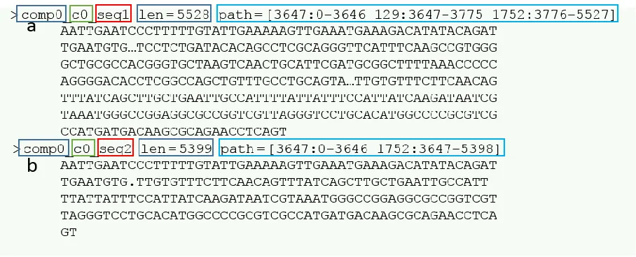
algorithm (Fig. 1). Each transcript name provides details regarding how the transcript was

reconstructed based on Chrysalis’s component ID (comp#), butterfly’s disconnected subgraph ID

(c#), and a final sequence identifier (seq#) (Haas et al., 2013). The combination of comp# and

c# can be interpreted as a gene, and seq# as an isoform of that gene. Throughout the course of

this body of work a transcript is defined to refer to either a gene or an isoform and will be used

[image:16.612.72.526.395.579.2]

unless a higher resolution is required.

(17)

Page | 16

to b) seq2. In addition here we can see that the splice variant, or isoform seq2, does not contain sequence information from node 129 (Haas et al., 2013).

Once Trinity assemblies have been generated they can be used as reference

transcriptomes to identify differentially expressed transcripts. The differential expression

pipeline first estimates expression levels for each sample using RNA-Seq by

Expectation-Maximization (RSEM) by aligning the clean reads to a reference transcriptome. Initially,

rsem-prepare-reference invokes bowtie2-build for the generation of the indexed transcriptome. The

rsem-calculate-expression command is then executed to invoke bowtie2 for single-end, strand

specific clean reads for the alignment of short clean reads to the indexed reference. Once the

alignments are complete the algorithm calculates the maximum likelihood expression values

using the previously generated alignments and the expectation-maximization statistical model (Li

and Dewey, 2011). The output is a tab delimited matrix file of transcript abundance estimates by

individual sequenced. These estimates are non-integer values representing the number of

fragments derived from a specific gene or isoform (Li and Dewey, 2011). All raw transcript

estimate matrices are then merged into one matrix file following the same layout describe for

individual matrix files.

Following the generation of transcript abundance estimates edgeR is invoked to identify

and analyze differentially expressed transcripts. Within edgeR pairwise comparisons are

executed between conditions using the quantile-adjusted conditional maximum likelihood

(qCML) method. This method relies on the implementation of the estimateCommonDisp() and

estimateTagwiseDisp() functions to generate common dispersion and tag dispersion statistics.

Finally differentially expressed transcripts are identified using the exactTest() and topTags()

(18)

Page | 17

than an user defined significance level. In addition to the identification and analysis of these

transcripts, edgeR can be utilized to assess the Biological Coefficient of Variant (BCV) for a

given experiment. This technique is implemented to characterize or assess the amount of

biological variation present between replicates. In addition, Multidimensional scaling (MDS) can

assist the user to visualize the scatter or dispersion of samples also providing key insights into

replicate relatedness.

Normalization methods are critical in comparing transcript abundances between samples

within an RNA-seq experiment. The TMM (trimmed mean of M-values) normalization approach

enables the comparison of transcript expression levels across multiple samples by accounting for

differences present in total RNA production levels across all samples (Haas et al. 2013). More

specifically, the TMM approach converts relative transcript abundance estimates to absolute

measures. The TMM normalized factor is defined as the ‘weighted mean of log ratios’ between

the test samples and an arbitrarily selected reference sample (Dillies et al., 2013). A ‘TMM

factor’ can be computed for all samples and is used to calculate effective library sizes which is

then used to transform FPKM transcript counts for downstream analyses. The definition of

library size can encompass the number of total expressed transcripts along with these transcript

lengths. This normalization method can correct for false-positives without the loss of statistical

power and can handle libraries of variable size and RNA composition (Dillies et al., 2013). The

false-discovery rate (FDR) is regarded as one of the least stringent multiple-test correction

methods, but when coupled with the TMM normalization method false-positives can be

corrected for in multiple steps.

The RNA-seq analyses implemented throughout this study was designed differently from

(19)

Page | 18

maximize biological variability derived from loci away from the Ren4 locus. Individual

seedlings were unreplicated, but all Ren4-resistant seedlings were combined to form

pseudo-replicates for comparison to all susceptible seedlings, resulting in abundant genetic variation

away from the locus, with the expectation of reproducible expression near the Ren4 locus.

Overall, we hypothesized that the integration of genetic, transcriptomic, and genomic

data would enable a detailed characterization of the Ren4 resistance locus providing insight into

key components of the resistance mechanism in grapevine.

Methods

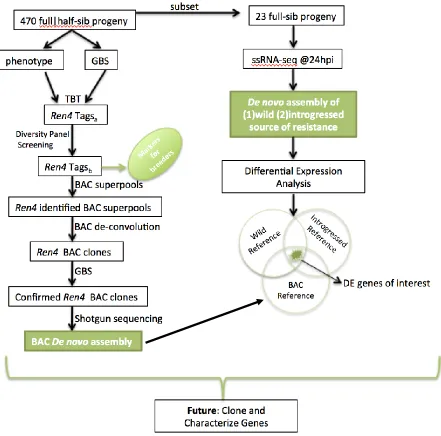
The scope of the thesis research is summarized in Figure 2. Analytical techniques were

completed on a USDA Linux machine with 24 cores, 32GB RAM, and 3TB HDD. Memory

intensive computations were carried out on a Linux machine with 64 cores, 512GB RAM and a

(20)

[image:20.612.79.520.76.512.2]

Page | 19

Figure 2. Experimental Flow Diagram detailing experimental methods and technologies to be

used for identifying the Ren4 locus. Expected deliverables noted in green.

Plant Material

As described previously, the ARS-Parlier breeding program has developed a series of

(21)

Page | 20

seedlings, segregating for Ren4 was developed from two resistant full-sibling parents (C87-41

and C87-14) each cross-hybridized to susceptible V. vinifera parents (Ramming, et al., 2010).

Each of these 470 progeny was phenotyped for powdery mildew resistance across multiple years

and was sampled for GBS, all prior to this research project. In addition, a subset of these

progeny, composed of 23 full-sibling grapevines were sampled in replicate for laboratory

inoculation, phenotyping, and RNA-sequencing during this project. As previously described,

Ren4 resistance was qualitative and summarized as susceptible (0) and resistant (1) for the

purpose of the following analyses. One replicate leaf for each individual was harvested 24hpi to

identify transcripts expressed in response to the onset of infection with an RNA-sequencing

approach. The remaining replicate leaf was harvested 7dpi in order to collect phenotype data

regarding the severity of infection in terms of sporulation and percent powdery mildew coverage

across the leaf surface. Results of the phenotypic data collection confirmed phenotypic data

collected within the field.

Ren4 enriched Tag Identification

A custom Perl program was developed to parse a 7.6 GB TBT file containing all Tags

generated for the 470 seedlings. Candidate Tags were selected based on two thresholds to limit

output Tags based on their uniqueness: at least 9:1 ratio enrichment for resistant to susceptible

Taxa (R:S) and requiring support from at least 10 resistant Taxa (Fig. 2). Candidate Tags were

then queried against a diversity panel of 6,851 grape accessions to remove Tags not fully

associated to the Ren4 resistant locus, ie present in germplasm unrelated to Ren4.

To fully characterize the source of Ren4 resistance present within V. romanetii, BAC

clones were generated prior to this project to capture genomic fragments arbitrarily distributed

(22)

Page | 21

generated using either BamHI or HindIII, each with 5X genomic coverage and distributed in

fifty-four 384-well plates. Each library was cloned into a BAC construction vector

pINDIGOBAC-5 specific to the restriction sites. The average insert size of V. romanetii DNA

was estimated as 128Kb for the BamHI library and 150Kb for the HindIII library. Row, column,

and plate superpools were generated combining multiple clones based on an orthogonal pooling

for subsequent GBS analysis. Plate superpools are simply all 384 BAC clones from one plate

pooled together in one well. Thus, there are 108 total plate superpools. Each row or column

superpool is composed of a single row or column from about 14 consecutive plates. Thus, a

superpool consists of 1 row of 24 wells from 14 consecutive plates. Therefore, within one

row-superpool there are 336 pooled BAC clones. Similarly, column-row-superpools are composed of 1

column of 16 wells from each of 14 plates, and each column-super pool consists of 224 pooled

BAC clones. Thus, each individual clone is present in one plate superpool, one column superpool

and one row superpool.

The presence of a DNA marker in three orthogonal superpools can be used to infer the

source well by deconvolution, or triangulation. To assist manual deconvolution, a correlation

matrix of R2 values was calculated for each pair of BAC clones, based on which GBS tags were

present in each clone. Clones with R2_{≥0.25 were grouped together for visual inspection. The}

simplest deconvolution was for clones with three GBS tags representing a unique

plate-row-column location. These were identified first and selected for BAC sequencing. Then clones

with six GBS tags representing two unique locations (two plates, two rows, two columns) were

identified. If a unique location had already been identified for one set of coordinates, a unique

location for the second clone could be inferred. If not, then eight wells could possibly contain

(23)

Page | 22

approach, any time we could deconvolute to 8 or fewer clones, we selected those for BAC

sequencing.

BAC Sequencing and Quality Control

All multiplexed Illumina libraries were submitted for sequencing on an Illumina HiSeq or

MiSeq at the Genomics Facility at Cornell University. Prior to sequencing all multiplexed

libraries were evaluated on the BioAnalyzer to evaluate the integrity of the samples regarding

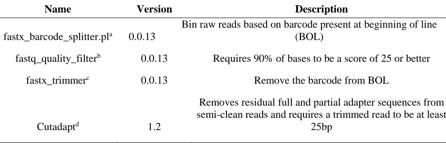
quality and quantity. Raw data was processed using a custom-built quality control pipeline

(qc-pipeline) utilizing publically available tools listed in Table 2. To elucidate the effectiveness of

the qc-pipeline the quality of a subset of samples were evaluated using FastQC before and after

the qc-pipeline, with an emphasis on nucleotide distribution, quality score distribution, and kmer

profile. All samples contain a 5 nucleotide barcode, followed by an ‘A’ as required by the T/A

ligation method to attach the barcode to any sequence contained within the library. This barcode

is utilized within the first phase of the qc-pipeline for demultiplexing and is subsequently

removed from the demultiplexed sequences (Table 2). A summary file was generated for each

lane to detail the read counts before and after quality control. The qc-pipeline resulted in high

[image:23.612.74.534.564.712.2]

quality, analysis-ready reads (clean reads).

Table 2. Tools included within the qc-pipeline. Tools a-c are all part of the FastX-Tool Kit developed by Hannon Lab, Cold Spring Harbor Laboratory (2008). Cutadapt was developed by Marcel Martin, MIT (2011).

Name Version Description

fastx_barcode_splitter.pla _0.0.13

Bin raw reads based on barcode present at beginning of line (BOL)

fastq_quality_filterb _0.0.13 _{Requires 90% of bases to be a score of 25 or better}

fastx_trimmerc _0.0.13 _{Remove the barcode from BOL}

Cutadaptd _1.2

Removes residual full and partial adapter sequences from semi-clean reads and requires a trimmed read to be at least

(24)

Page | 23

a_{–exact; –BOL; –suffix .fq} b _{-Q33; –q 25; –p 90} c _{-Q33; –f 7}

d _{–a; –minimum-length 25; –O 6}

BAC Assembly

Following the qc-pipeline, estimated depth of coverage was computed for each restriction

enzyme used to generate the BACs. A fully automated python script was developed to

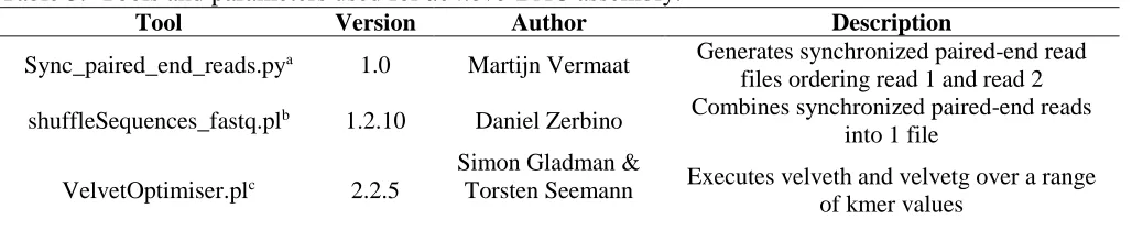
iteratively assemble all BAC clones. The pipeline is detailed in Table 3 and utilizes

sync_paired_end_reads.py (Martijn Vermaat), shuffleSequences_fastq.pl, and

velvetOptimiser.pl. Velvet optimizer is a wrapper script developed to generate an optimal

assembly using Velvet. The optimizer tool takes a variety of command line parameters including

–s and –e which represent the lower and upper bounds for kmer length, respectively. In addition,

a hash step size of 4 was defined with the –x parameter (Table 3). With these parameters the

optimizer tool generates assemblies using kmer hash length of 149-250 with a step size of 4bp to

find the assembly with the largest N50 value (Table 3).

Velvet Optimiser computes a variety of quality metrics along with the final assembly.

Final assemblies are selected based on their length of total assembly, length of longest contig,

[image:24.612.72.586.578.683.2]

number of contigs, and N50 value.

Table 3. Tools and parameters used for de novo BAC assembly.

Tool Version Author Description

Sync_paired_end_reads.pya _1.0 _{Martijn Vermaat} Generates synchronized paired-end read

files ordering read 1 and read 2

shuffleSequences_fastq.plb _1.2.10 _{Daniel Zerbino} Combines synchronized paired-end reads

into 1 file

VelvetOptimiser.plc _2.2.5

Simon Gladman &

Torsten Seemann Executes velveth and velvetg over a range of kmer values

a _{1.fq; 2.fq; Sync_1.fq; Sync_2.fq;}

(25)

Page | 24

c _{-s 149; -e 250; -x 4; -t 8; -p}

MUMmer version 3.23 was used to evaluate the physical positions of all BAC contigs using

the parameters detailed in table 4. The minimum match length parameter (-l) was defined at

200bp to ensure a significant match was observed but relaxed enough to take species divergence

into consideration between V. romanetii and V. vinifera (Table 4). In addition, sequence

information for the SSR marker PN18-01, a marker co-located with the Ren4 region, was used to

provide a point of reference. A perl script was developed to parse the non-uniform mummer

output into a more user-friendly, tab delimited document easily imported into excel for the

[image:25.612.114.498.352.434.2]

generation of BAC contig distribution plot.

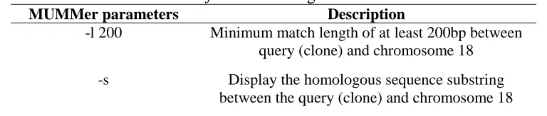
Table 4 | MUMMer command line parameters used for aligning BAC contigs to the Vitis vinifera reference genome.

MUMMer parameters Description

-l 200 Minimum match length of at least 200bp between query (clone) and chromosome 18

-s Display the homologous sequence substring between the query (clone) and chromosome 18

BAC Scaffolding and Fragmentation

Vector and contaminate sequences were trimmed or removed from individual BAC

assemblies using SeqClean and the UniVec database (NCBI). A total of 1790 contigs, from all

111 BAC clones, were processed by SeqClean resulting in 1755 trimmed sequences and 35

discarded sequences. A scaffolded assembly was generated using SSPACE_Basic_v2.0 with a

variety of user defined command line parameters (Table 5).

Table 5 | SSPACE implemented command line parameters for scaffold generation from pre-assembled Velvet contigs.

SSPACE parameters Description

(26)

Page | 25

-s FASTA file of all SeqCleaned contig sequences

-m 50; This value is the minimum number of overlap required between a seed and a contig.

-k 5; Number of paired-end reads to support a scaffold

-g 3; Gaps allowed during bowtie alignments

*Information was held consistent for all BAC clones. Insert size = 650bp; Error rate= 0.95; strand specificity= FR; Insert size can be defined as the expected length of sequence information contained in between paired-end reads. The error rate allows for a level of deviation to be

tolerated in this expected insert size estimate. Thus, if our expected insert size is 650 and an error rate of 0.95 our acceptable range is 33bp-1267bp.

The BAC scaffolds were used as a reference for RNA-Seq analysis. Rather than annotate

gene sequences in the scaffolds and introduce annotation errors, such as by missing truncated

genes at the end of a contig, a custom Perl script was used to disassociate the BAC assembly into

1kb fragments. Fragments were named with their source scaffold name concatenated with the

fragment number 0...n, where n is the number of fragments generated

RNA-Sequencing and Quality Control

The RNA-sequencing was accomplished by the generation of cDNA libraries prepared

using a strand-specific approach with custom barcoded adapters (Zhong et al., 2011).

Multiplexed libraries were then subjected to single end (SE) Illumina HiSeq sequencing with

100bp raw reads. Deep sequencing was executed for both the wild (NY19-91) and introgressed

resistance (y302_183) sources of Ren4 resistance through the utilization of both paired-end (PE)

2x250bp Illumina MiSeq and PE 2x150bp Illumina HiSeq sequencing. The qc-pipeline was

executed on all RNA-seq raw reads with previously defined parameters (Table 2).

Trinity de novo Assembly

For de novo transcriptome assembly using the hybrid approach, the clean reads from

MiSeq and HiSeq were concatenated into one file per individual, NY19-91 or y302_183. Trinity

(27)

Page | 26

their respective values were selected based on experiment design and previously published data

(Table 6) (Haas et al., 2013). Quality statistics were generated using the TrinityStats.pl script

provided by the developers. For each transcriptome, clean reads were aligned back to their

[image:27.612.69.541.270.376.2]

respective assembly using the align_reads_to_assembly.pl script.

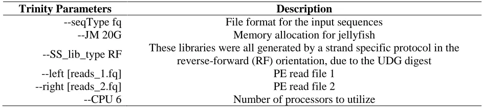
Table 6 | Displays the command line parameters given to trinity for both de novo transcriptomes. The –left and –right parameters were specific to what assembly was being created, all others were held constant See Zhong, et al. 2011 for more details regarding the UDG digest method for strand-specific library preparation. For a more detailed explanation of all Trinity parameters see http://trinityRNA-seq.sourceforge.net/ (Haas et al., 2013)

Trinity Parameters Description

--seqType fq File format for the input sequences

--JM 20G Memory allocation for jellyfish

--SS_lib_type RF These libraries were all generated by a strand specific protocol in the reverse-forward (RF) orientation, due to the UDG digest

--left [reads_1.fq] PE read file 1

--right [reads_2.fq] PE read file 2

--CPU 6 Number of processors to utilize

Differential Expression Analysis

For the identification of differentially expressed transcripts, a semi-automated command

line protocol was followed (Haas et al., 2013). Read alignment and abundance estimation was

executed using run_RSEM_align_n_estimate.pl on all clean reads (Workflow 1). Transcript

abundance estimates were generated for each sample and merged using

merge_RSEM_frag_counts_single_table.pl into one matrix containing abundance estimates for all

transcripts expressed within each sample.

To characterize the BCV of the experiment, data was reduced to only transcripts with

counts per million (cpm) > 100 and present in 10 or more individuals. MDS plot was generated to

visually describe the data for one reference transcriptome.

Differentially expressed transcripts were identified using run_DE_analysis.pl (Workflow

(28)

Page | 27

library to define the average library size observed throughout all samples (Dillies et al., 2013).

Significant differentially expressed transcripts are identified using analyze_diffexpr.pl. Nomial

and FDR corrected p-value plots were constructed for each transcriptome to define alpha, α, for

identifying significant differentially expressed transcripts. All command line parameters used

(29)

Page | 28

(30)

Page | 29

Candidate Evaluation

There are a variety of characteristics that would make a differentially expressed transcript

an ideal candidate as a Ren4 resistance gene: (1) statistically significant differential expression

with a high fold-change, (2) the physical mapping of the transcript to the Ren4 locus, based on

the V. vinifera PN40024 reference genome, (3) the presence of the candidate within the

scaffolded BAC assembly, and (4) a functional annotation of a role in disease resistance. The

collection and integration of these data was conducted to identify candidates for cloning and

functional characterization.

Following DE analysis, transcripts are selected for annotation if they satisfy the following

two criteria such as FDR corrected p-value ≤ = 1.0x10-3 and a FPKM expression ratio ≥ 30

(resistant vines to susceptible vines). All identified transcripts, meeting these criteria, were

extracted from their respective reference transcriptome indexes using a custom Perl script. This

script requires three command line arguments to be defined (1) the indexed reference

transcriptome, (2) a list of candidate names for extraction, in agreement with the naming scheme

within the indexed reference, and (3) an output FASTA file name that the script will populate

with sequence data. BLAT v.34 was then used to assess the physical positioning of these

candidates within PN40024 and the scaffolded BAC assembly. The resulting output file was in

the “.psl” format and was parsed for a variety of characteristics including query

mismatches/matches, length, start/stop coordinates and source chromosome/node from the

reference material. To support a candidate as a Ren4 resistance gene, we required the transcript

to align with chromosome 18 (PN40024) near the Ren4 locus, defined as being between

30Mb-34.5Mb. The presence of the candidate within the scaffolded Ren4 BAC assembly further

confirmed the location and provided information regarding regulatory regions useful for

(31)

Page | 30

For cloning and functional characterization, ten candidate transcripts could reasonably be

pursued with the resources available. Identifying this small number of elite candidate transcripts

required data summarization, interpretation, and selection of objective thresholds. Following

summarization of the above data, the best candidates for functional characterization met the

following requirements: FDR ≤ 0.001, FPKM expression ratio ≥ 30 (resistant vines to

susceptible vines), homology ≥ 125bp with either a Ren4 BAC scaffold or PN40024 reference

genome on chromosome 18 around the locus 30Mb-34.5Mbp.

A custom Perl program was developed to extract candidates from the scaffolded BAC

assembly with additional +/-4Kb flanking the candidate transcript, allowing for the isolation of

the full-length gene and native promoter for cloning and functional characterization.

The last phase in selecting top candidates for cloning was functional annotation using

Blast2go. Blastx was used internally within blast2go to annotate a FASTA file containing

previously selected candidate transcripts against the non-redundant NCBI database. A blast

expect threshold value of 1.0E-3 was set and 20 blast hits were collected for each candidate and

reported in the XML format. GO-Mapping and InterPro-Scan were also executed following

default parameters.

Results

Ren4 enriched Tag Identification and BAC Selection

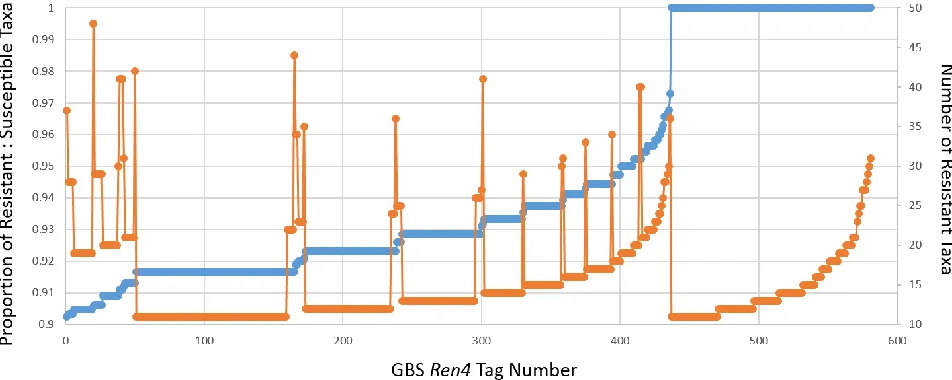
From 471 full- and half-sib progeny segregating for Ren4 introgressed into a V. vinifera

background, 581 tags were found to be associated with resistance (Fig 4). A diversity panel of

6,851 Vitis accessions was screened for the presence of these 581 tags, and 70 tags were found

only in Ren4-related germplasm. The remaining 511 tags were frequently found in V. vinifera

(32)

[image:32.612.79.555.80.270.2]

Page | 31

Figure 4 | Displays preliminary results of the 581 tags regarding association with resistant taxa. The primary axis (blue) displays the proportion of resistant taxa associated with each Tag. The secondary axis (orange) displays the total number of Resistant Taxa associated with each tag.

The use of these 70 Tags to deconvolute the BAC superpools resulted in a total of 111

clones selected for sequencing. A total of 33 BACs were deconvoluted with high certainty and

probability given that a GBS tag occurred in a unique plate, row, and column superpool. The

remaining 78 clones had uncertain deconvolution such that we selected 2 to 8 clones from which

there should be one true positive Ren4 BAC. Given this redundancy, of the 111 selected clones,

about 50 were expected to match the Ren4 locus and the rest to be arbitrarily distributed across

the genome.

BAC Sequencing and Quality Control

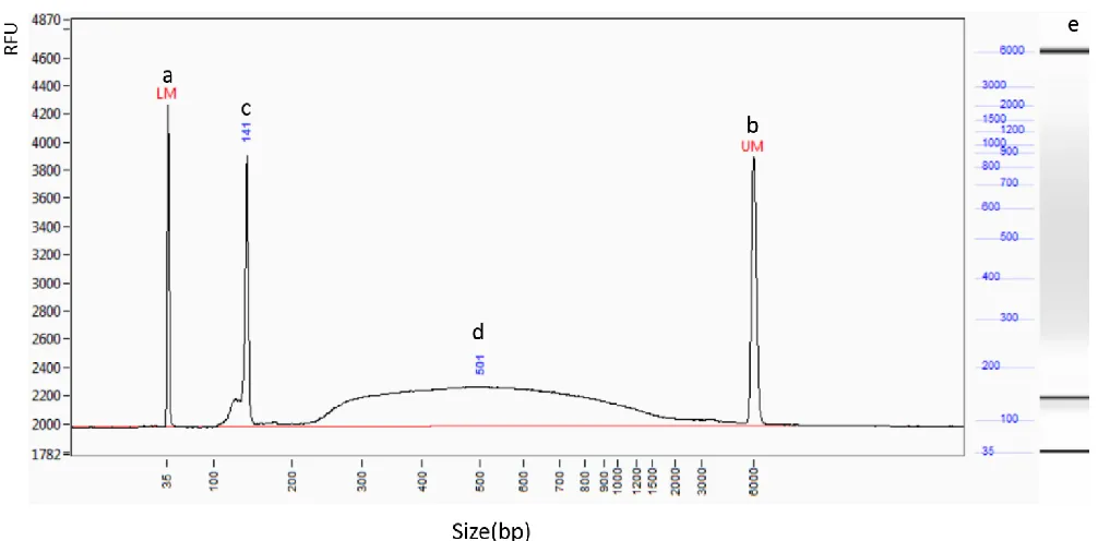
BioAnalyzer evaluation resulted a fragment analysis summary report containing

information regarding the integrity of the multiplexed library (Fig 5). The results illustrate an

adapter dimer peak with a size of 141bp with an intensity of 3900RFU which can be removed

prior to sequencing (Fig. 5c). A broad smear of BAC fragments for Illumina sequencing can be

(33)

[image:33.612.76.579.86.334.2]

Page | 32

Figure 5 | Fragment Analyzer run summary provided by Cornell’s sequencing facility, regarding one multiplexed BAC Illumina library. The y-axis displays the intensity of the DNA peak in RFU and the x-axis displays the size of the DNA fragments in bp a) The lower bound size standard at 35bp. b) The upper bound size standard at 6kb. c) Undesirable adapter dimer, which can result during the ligation phase of the library generation, at 141bp. d) Broad smear of fragments containing randomly sheared DNA from the BAC clones ranging from 250bp-3kb with the highest quantity of fragments at 501bp. e) Alternative illustration of the results indicating size on the left hand side and a electrophoretic gel simulation on the right, showing how the previously mentioned fragments migrated.

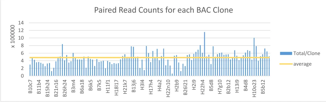
The qc-pipeline resulted in an average of 482,877 clean reads per clone (Fig. 6). Clone

B26h21 had the least amount of sequencing depth with only 61,163 clean reads whereas B12j6

had the greatest sequencing depth of 811,599 clean reads (Fig. 6). On average, 23% of raw reads

were lost throughout the qc-pipeline. Clones with low clean read counts, such as B26h21, had

additional quality issues in the raw reads. For example, B26h21 nucleotides throughout the first

half of the raw reads had an uneven nucleotide distribution (Fig. 7-Raw reads). Raw nucleotide

distributions of moderate and high-sequenced clones show uniformity across the read for all

(34)

Page | 33

site (Fig.7-Raw reads). All nucleotide distributions indicated that, regardless of sequencing

depth, quality of some raw reads began a linear decline after 140bp (Fig. 7). Thus, after quality

trimming approximately 50% of the reads retained high quality scores throughout the 250bp read

length (Fig. 8-Clean reads). The quality score plot also illustrates that the overall quality of

B26h21 (with low read count) was overall much lower and more variable compared to the

medium and highly sequenced library (Fig. 8). Overrepresented kmer sequences were present in

all raw libraries regardless of read count (Fig. 9). The presence of overrepresented kmer

sequences is eliminated by the qc-pipeline (data now shown). On average, all HindIII and

[image:34.612.71.590.331.494.2]

BamHI libraries were sequenced to 810x and 665x coverage, respectively (Table 7).

Figure 6 | Clean paired-read count for each BAC Clone. Details the paired-end read counts for each BAC clone library within one lane of sequencing. Each pair is graphed separately to illustrate the variation in read counts between R1 and R2 files. The average read count is indicated in yellow around ~5k clean reads/clone.

0 2 4 6 8 10 12 14 B10c 7 B11b 4 B15h 24 B21n 16 B26h 24 B3m 4 B6a 18

B6k5 B7k5 _H11f1

H

18l

17

H

21k7 _B13j6 H3l

4 H17h 4 H 4a2 H 22n 10 H 2b 9 B26l21 H 2i 9 H 22h 4

B5d8 _H7g10

B2b1 2 H 13i 9 B4d 8 H 10o 23 B5b1 2 x 1000 00

Paired Read Counts for each BAC Clone

Total/Clone

(35)

[image:35.612.86.539.77.521.2]

Page | 34

(36)

[image:36.612.82.532.75.572.2]

Page | 35

(37)

[image:37.612.162.454.76.590.2]

Page | 36

(38)

[image:38.612.80.505.473.715.2]

Page | 37

Table 7 | Displays average insert size, expected read length and estimated coverage for all BAC clones created with the HindIII and BamHI restriction enzymes.

a_{Restriction enzyme utilized to digest the genomic}_{DNA for generation of BAC clones.} b _{Average Read Count/Clone is the average number of clean reads per clone.}

c _{Average Insert Size the average expected size in nucleotides (nt) of the genomic material}

contained within a given BAC.

d_{Expected Read Length is the expected MiSeq raw read length.} e_{Observed Read Length is the average clean read length.}

f_{Observed Coverage is defined as: (observed read length x average read count/clone)/average}

insert size.

BAC Assembly

The assembly results for a subset of clones is shown in Table 8. On average, the kmer

value that generated the optimal results was 214 (Table 8), resulting in a total of 1,789 BAC

nodes across all clones. Contig N50 values ranged as low as 11,347nt to as high as 68,076nt. The

average total length of the subset displayed is 121,600nt. The average N50 value across all 111

clones was 25,037nt.

Table 8 | Assembly statistics for a subset of clones assembled using Velvet Optimizer.

Clone Kmera _{Total Nodes}b _{N50 (nt)}c _{Max Length (nt)}d _{Total Length (nt)}e

B10d7 221 16 14,046 34,005 109,531

B10c7 221 11 26,309 41,739 106,374

B10m7 217 12 29,253 43,488 121,025

B11b4 201 8 40,627 53,492 141,124

B11b12 213 4 68,076 68,076 123,982

B12j6 213 18 17,531 29,182 116,873

B12j10 213 22 11,347 20,032 132,288

H10c1 225 19 19,203 21,883 140,854

H10o23 225 22 20,314 32,455 158,334

H13b8 213 46 11,713 29,330 200,908

H13b9 205 24 13,361 25,365 126,873

H13i8 213 10 17,537 23,662 128,990

H13i9 205 38 47,525 96,731 224,590

H14c6 213 24 67,287 71,673 181,862

H7g10 213 10 40,087 51,333 125,004

Restriction Enzyme a

Average Read Count/Clone b

Average Insert Size c

Expecte d Read Length d

Observed Read Length e

Expected Coverage f

Observed Coverage g

(39)

Page | 38

Average 214.1 18.9 29,614.4 42,829.7 142,574.1

a_{Kmer shows the optimal values in nucleotides (nt) identified during Velvet Optimiser.} b_{Total nodes represents the total number of contigs contained within the assembly.} c_{For N50, the majority of observed contigs is this reported size or larger.}

d_{Max Length is the largest reconstructed contig within the assembly.} e_{Total Length is the nucleotide sum of all assembled contigs for that clone.}

Aligning the above 1,789 BAC nodes against the PN40024 chromosome 18 there were

1,130 homologies at least 200bp in length. Of these 1,130 homologies, 719 of them were present

within the Ren4 locus defined broadly as 25Mb-34.5Mbp (Fig. 10). There was a total of 76 BAC

clones that had homology with chromosome 18 and 35 clones that did not share homology with

[image:39.612.77.574.346.561.2]

chromosome 18.

(40)

Page | 39

BAC Scaffolding and Fragmentation

The scaffolding process of all contigs of all clones resulted in 1,413 scaffolds totaling

13.7Mb (Table 9). The maximum, minimum, and average scaffold size was 112,994nt, 166nt,

and 9,720nt respectively (Table 9). SSPACE records Contig N50 values throughout the

[image:40.612.75.542.333.381.2]

algorithm, after the incorporation of additional previously assembled contigs, and are shown in

Fig. 11. The N50 of the final scaffolded assembly was 24,740nt (Table 9). Scaffolded BAC

assembly fragmentation for alignment of RNA-Seq reads resulted in a Pseudo-transcriptome

[image:40.612.74.526.379.654.2]

with 14,371 pseudo-transcripts ≤1kb in length.

Table 9 | Displays total number of scaffolds, sum length (bp), maximum scaffold size, minimum scaffold size, average scaffold size, and N50 value for the Scaffolded BAC Assembly of 111

clones.

Total Number

of Scaffolds Sum (nt)

Max Scaffold Size (nt)

Min Scaffold Size (nt)

Average Scaffold sizeSize (nt)

N50 (nt)

1,413 _13,734,859 _112,994 ₁₆₆ _9,720 24,740

(41)

Page | 40

Figure 11 | Reported contig N50 values while iteratively incorporating previously assembled BAC contigs from the 111 clones into the scaffolded assembly. The initial reported N50 was 18,047nt and the final contig N50 value was 24,740nt an overall improvement of 6,693nt.

RNA-Sequencing and Quality Control

RNA-Seq data was collected for 23 F1 seedlings and two genotypes for the generation of

de novo transcriptomes. Illumina HiSeq 1x100bp sequencing resulted in an average of 5.2M

clean reads per seedling, ranging from 590,614 to 13,442,689 (Fig. 12a). On average, 30% of

raw reads were lost per individual throughout the course of the QC-pipeline.

During deeper sequencing of two samples for development of reference transcriptomes, a

technical artifact of Illumina HiSeq 2x150 sequencing resulted in the loss of many R1 reads. A

total of 92.8% and 85.4% of R1 reads were lost during the QC-pipeline for y302_183 and

NY19-91 respectively, versus 47.8% and 33.5% of R2 reads. This resulted in unbalanced read depth

(Fig. 11) and many unpaired reads. Illumina MiSeq 2x250 sequencing of the same individuals

produced balanced results with approximately 35% of reads lost during the QC-pipeline for both

R1 and R2 reads for both individuals. All paired reads for the two sequencing technologies were

combined to produce 49.2M and 57.8M reads for y302_183 and NY19-91, respectively (Fig.

(42)

[image:42.612.83.582.74.418.2]

Page | 41

Figure 12 | RNA-seq read counts across all seedlings. (a) Single end clean read counts for each seedling within the segregating population. The orange horizontal line shows the average read count of 5.2M reads. (b) Paired-end MiSeq and HiSeq clean read counts for each genotype used for de novo transcriptome assembly. All R1 read counts are illustrated in blue and all R2 read counts are in orange.

Transcriptome Assembly

The combined paired-end reads were used in Trinity for de novo transcriptome assembly.

Trinity descriptive statistics provided information regarding transcripts, components, and contig

N50 (Table 10). Mapping all input clean reads (HiSeq and MiSeq) resulted in right only (R2)

reads being the highest proportion of reads aligning to the reference transcriptome (Table 10c/d).

The second highest classification for reads mapped back was “proper pairs” or concordant read

pairs, at 25.78% and 22.96% for NY19-91 and y302_183, respectively (Table 10c/d). The final

(43)

Page | 42

MiSeq clean input reads resulted in the highest proportion of improper pairs to align to the

[image:43.612.57.583.327.670.2]

reference transcriptome (Table 10e/f).

Table 10 | Assembly and quality evaluation statistics regarding Trinity-assembled de novo transcriptomes a) Number of trinity assembled transcripts and components along with Contig N50 b) Number of trinity assembled transcripts and components along with Contig N50 c) All input clean reads, 2x150 HiSeq and 2x250 MiSeq mapped back to reference transcriptome, NY19-91, results including right only, proper pairs, improper pairs, and left only reads d) All input clean reads, 2x150 HiSeq and 2x250 MiSeq mapped back to reference transcriptome, y302_183, results including right only, proper pairs, improper pairs, and left only reads e) Only 2x250 MiSeq clean reads mapped back to reference transcriptome, NY19-91, results including right only, proper pairs, improper pairs, and left only reads f) Only 2x250 MiSeq clean reads mapped back to reference transcriptome, y302_183, results including right only, proper pairs, improper pairs, and left only reads

NY19-91 y302_183

a b

Transcripts 156,525 Transcripts 135,146

Components 89,644 Components 76,921

Contig N50 2,104bp Contig N50 1,716bp

2x150 HiSeq & 2x250 MiSeq

c d

Read Type Count Percent (%) Read Type Count Percent (%)

Right only 67,245,243 50.58 Right only 51,478,060 54.26

Proper pairs 34,273,202 25.78 Proper pairs 21,783,860 22.96

Improper pairs 24,107,716 18.13 Improper pairs 15,782,310 16.64

Left only 7,328,422 5.51 Left only 5,821,550 6.14

2x250 MiSeq

e f

Read Type Count Percent (%) Read Type Count Percent (%)

Right only 4,940,420 14.07 Right only 4,73,075 11.64

Proper pairs 5,707,010 16.26 Proper pairs 9,621,500 25.61

Improper pairs 20,890,004 59.51 Improper pairs 19,404,586 51.65

Left only 3,566,721 10.16 Left only 4,173,600 11.11

(44)

Page | 43

Differential Expression Analysis

Twenty-three seedlings were sequenced using a strand-specific RNA-Seq approach, and

clean reads were aligned to the y302_183 and NY19-91 reference transcriptomes as well as to

the BACfrag pseudo-transcriptome reference. On average 36,160 and 60,657 (genes/isoforms)

were expressed using the y302_183 transcriptome; 35,513 genes and 57,575 isoforms were

expressed using the NY91-19 transcriptome; 4051 of 14,371 BAC fragments were expressed.

Not including Y302_183, there was a nearly perfect correlation between the number of genes or

isoforms expressed in the two reference transcriptomes (R2>0.998, Fig. 13a). The outlier to the

right of each line shows the values for Y302_183, which had more transcripts identified when

aligned to its own reference transcriptome than when aligned to NY19-91. Regressing the

isoforms versus the genes for each assembly also showed a nearly perfect correlation (R2_>0.997),

and the slope suggested that there are 1.8 expressed isoforms per expressed gene, regardless of

(45)

[image:45.612.151.497.76.488.2]

Page | 44

Figure 13 | Correlation of transcript alignments across seedlings. For each seedling, clean RNA-Seq reads were aligned to NY19-91 and Y302_183. Each data point shows for a single seedling the number of transcripts (genes or isoforms) having aligned reads. A) the regression of NY19-91 versus Y302_183 shows the similar results from the two references. The outlier to the right of each line shows the values for Y302_183, which was not included in the regression

calculations, since it was also a reference transcriptome. B) the regression of isoforms versus genes shows the reproducible number of isoforms per gene across both assemblies.

Nominal and FDR corrected p-value plots display an exponential phase and a linear

phase (Fig. 14) that suggested significance thresholds at the inflection points, typically around

(46)

Page | 45

nominal p-value > 1.0x10-3 were observed in the linear phase (Fig. 13), so this value was used as

[image:46.612.155.457.131.569.2]

a conservative significance threshold for subsequent analyses.

Figure 14 | Nominal (blue) and FDR-corrected (orange) p-value plots for differentially expressed transcripts for three reference transcriptomes on a logarithmic scale of p-values. Differentially expressed transcripts identified aligning to the a) y302_183 reference

transcriptome, b) NY19-91 reference transcriptome, and c) BACfrag pseudo-transcriptome.

The raw data was filtered to capture transcripts broadly expressed in all individuals. This

(47)

Page | 46

of the filtered population illustrates a randomly dispersed pattern of F1 progeny (Fig.15). The

BCV on the filtered population is 0.4599. These results reflect the experimental design and goal

that the genome-wide variance within treatment should as great as the variance between

[image:47.612.70.539.178.562.2]

treatments.

Figure 15 | Multidimensional scaling plot of normalized FPKM expression valuesof all transcripts expressed within the segregating population when aligned to the y302_183 de novo transcriptome for transcript quantification.

(48)

Page | 47

Comparing resistant seedlings versus susceptible seedlings, 35 transcripts were differentially

expressed at an FDR threshold of α = 1.0x10-3_{. Of these 35 isoforms, 25 had an average}

resistant:susceptible (R:S) FPKM ratio ≥30. These 25 isoforms represented 17 unique genes.

The heat map dendrogram hierarchically clusters genotypes and transcripts based on expression

values that are log2 transformed and median centered (Haas et al., 2013). The columns and rows

of the heatmap represent samples and transcripts, respectively (Fig. 16). The expression pattern

of the differentially expressed transcripts correctly cluster the genotypes into two groups,

(49)

[image:49.612.130.490.64.549.2]

Page | 48

Figure 16 | Hierarchically clustered F1 seedlings (column) and differentially expressed

(50)

Page | 49

NY19-91

expressed at an FDR threshold of α = 1.0x10-3_{. Of these 28 isoforms, 19 had an average}

resistant:susceptible (R:S) FPKM ratio ≥30, representing 12 unique genes. Hierarchical

clustering of genotypes and transcripts based on log2-transformed, median-centered expression

values correctly clustered the genotypes into two groups, susceptible and resistant seedlings (Fig.

(51)

[image:51.612.137.483.68.548.2]

Page | 50

Figure 17 | Hierarchically clustered samples (column) and differentially expressed

(52)

Page | 51

BACfrag

expressed at an FDR threshold of α = 1.0x10-3_{. Of these 21 transcripts, 10 had an average}

resistant:susceptible (R:S) FPKM ratio ≥30. Hierarchical clustering of genotypes and transcripts

based on log2-transformed, median-centered expression values correctly clustered the genotypes

(53)

[image:53.612.115.487.64.589.2]

Page | 52

Figure 18 | Hierarchically clustered samples (column) and differentially expressed

(54)

Page | 53

Candidate Evaluation

Candidate evaluation focused on the differentially expressed transcripts identified within

the F1 population when aligned to the 2 de novo reference transcriptomes. Differentially

expressed transcripts identified with the BACfrag pseudo-transcriptome were not included in this

phase of candidate evaluation. In total, 44 isoforms were identified with an FDR p-value ≤

1.0x10-3_{and an R:S ratio of ≥ 30. A variety of additional requirements were implemented to}

further reduce the candidate pool: 1) homology to chromosome 18 of PN40024 within the Ren4

locus defined as 30Mb-35Mb, 2) homology with at least 1 BAC clone, and 3) functional

annotation. A phylogenetic analysis of all candidates reveals there are 3 instances of candidate

pairs when a candidate from each genotype transcriptome is identical (Fig. 19).

Of the 44 initial candidate isoforms, 31 were found on chromosome 18. Of these 31, 19

were found within the Ren4 locus. A total of 29 of the 31 candidates shared sequence homology

with an assembled BAC clone. Several of the initial 44 candidates were isoforms of the same

gene (based on sharing the same comp identifier and different seq IDs). One instance of each

gene was selected for annotation. Finally, all data was taken into account and 7 resistance genes

(55)

[image:55.612.119.498.71.666.2]

Page | 54

Characterization of the Ren4 resistance locus through the integration of de novo assembly, expression analysis, and Genotyping-by-Sequencing data

RIT Scholar Works

Characterization of the Ren4 resistance locus

through the integration of de novo assembly,

expression analysis, and

Genotyping-by-Sequencing data

Characterization of the

Ren4

resistance locus

through the integration of

de novo

assembly,

expression analysis, and

Genotyping-by-Sequencing data

Jacquelyn A. Lillis

Cadle-Davidson Lab (USDA-ARS)

A Thesis submitted in partial fulfillment of the requirements for the degree of

Master of Science in Bioinformatics

Department of Bioinformatics

College of Science

Rochester Institute of Technology

Rochester, NY

Contents

Methods

Results

Paired Read Counts for each BAC Clone