City, University of London Institutional Repository
Citation
: Kyriazis, N., Koukouvinis, P. ORCID: 0000-0002-3945-3707 and Gavaises, M.
ORCID: 0000-0003-0874-8534 (2018). Modelling cavitation during drop impact on solid
surfaces. Advances in Colloid and Interface Science, 260, pp. 46-64. doi:
10.1016/j.cis.2018.08.004
This is the accepted version of the paper.
This version of the publication may differ from the final published
version.
Permanent repository link:
http://openaccess.city.ac.uk/id/eprint/20484/
Link to published version
: http://dx.doi.org/10.1016/j.cis.2018.08.004
Copyright and reuse:
City Research Online aims to make research
outputs of City, University of London available to a wider audience.
Copyright and Moral Rights remain with the author(s) and/or copyright
holders. URLs from City Research Online may be freely distributed and
linked to.
City Research Online:
http://openaccess.city.ac.uk/
[email protected]
Modelling cavitation during drop impact on solid
surfaces
Nikolaos Kyriazisa,∗, Phoevos Koukouvinisa, Manolis Gavaisesa
aSchool of Mathematics, Computer Science & Engineering, Department of Mechanical
Engineering & Aeronautics, City University London, Northampton Square EC1V 0HB, United Kingdom.
Abstract
The impact of liquid droplets on solid surfaces at conditions inducing
cavita-tion inside their volume has rarely been addressed in the literature. A review
is conducted on relevant studies, aiming to highlight the differences from
non-cavitating impact cases. Focus is placed on the numerical models suitable for the
simulation of droplet impact at such conditions. Further insight is given from
the development of a purpose-built compressible two-phase flow solver that
in-corporates a phase-change model suitable for cavitation formation and collapse;
thermodynamic closure is based on a barotropic Equation of State (EoS)
repre-senting the density and speed of sound of the co-existing liquid, gas and vapour
phases as well as liquid-vapour mixture. To overcome the known problem of
spurious oscillations occurring at the phase boundaries due to the rapid change
in the acoustic impedance, a new hybrid numerical flux discretization scheme is
proposed, based on approximate Riemann solvers; this is found to offer
numeri-cal stability and has allowed for simulations of cavitation formation during drop
impact to be presented for the first time. Following a thorough justification of
the validity of the model assumptions adopted for the cases of interest,
numer-ical simulations are firstly compared against the Riemann problem, for which
the exact solution has been derived for two materials with the same velocity
∗Corresponding author
Email addresses: [email protected](Nikolaos Kyriazis ),
[email protected](Phoevos Koukouvinis),[email protected]
and pressure fields. The model is validated against the single experimental data
set available in the literature for a 2-D planar drop impact case. The results
are found in good agreement against these data that depict the evolution of
both the shock wave generated upon impact and the rarefaction waves, which
are also captured reasonably well. Moreover, the location of cavitation
forma-tion inside the drop and the areas of possible erosion sites that may develop on
the solid surface, are also well captured by the model. Following model
valida-tion, numerical experiments have examined the effect of impact conditions on
the process, utilising both planar and 2-D axisymmetric simulations. It is found
that the absence of air between the drop and the wall at the initial configuration
can generate cavitation regimes closer to the wall surface, which significantly
increase the pressures induced on the solid wall surface, even for much lower
impact velocities. A summary highlighting the open questions still remaining
on the subject is given at the end.
Keywords: Cavitation, drop impact, approximate Riemann solvers,
OpenFOAM
1. Introduction
Droplets impacting onto solid or liquid surfaces are of significant importance
in many engineering applications, oceanography, food science and even forensics;
see selectively [1, 2, 3, 4, 5, 6] among many others. For isothermal conditions,
the Weber We, Reynolds Re, Ohnesorge Oh and Froude Fr numbers are
fre-5
quently utilised to characterise the droplet impact outcome; these are defined
as We = ρlu2impD
σ , Re =
ρluimpD
µl , Oh =
√
We
Re and Fr = uimp
√
gD, respectively. In
these relations,uimp is the impact velocity normal to the wall surface,D is the
droplet diameter,µland ρl are the dynamic viscosity and density of the liquid
droplet respectively,σ is the surface tension andg is the gravitational
acceler-10
ation. A number of post-impact outcomes are known for the normal/inclined
impact of spherical droplets onto flat and smooth surfaces [7, 8]. In the vast
evo-lution of the droplet shape upon impact can be described assuming that the
liquid and the surrounding media behave as incompressible media. Still, out of
15
the very broad literature on the subject, or interest to the present paper are
the cases of impact at velocities of the order of 200m/s (M ≈ 0.6 for air at room temperature and atmospheric pressure) which are high enough for
com-pressibility effects to become important. Moreover, at such conditions pressure
waves developing within the liquid during impact may induce cavitation
for-20
mation within the droplet volume. Cavitation as a phenomenon involves the
formation of vaporous/gaseous cavities in the bulk of liquid, due to localized
static pressure drop. This can happen due to strong accelerations, high
veloci-ties or pressure waves. In the first case, cavitation is termed as ’hydrodynamic’
and may occur in any device operating with liquids, e.g. propellers, turbines,
25
pumps, valves etc. In the second case, cavitation is termed as ’acoustic’, since it
is induced by the presence or interaction of acoustic waves. Phase-change during
cavitation is inertial driven [3] as opposed to phase-change processes driven by
the temperature difference between the liquid, air and the solid surface.
More-over, for the high impact velocity conditions leading to cavitation formation,
30
the impact outcome is expected to be in the splashing regime, where a corona
is initially formed and gradually disintegrates into a number of droplet
frag-ments. Such impact velocities can be realised, for example, in steam turbines
and aircraft components. The steam in the turbine engine operating at low
pres-sure conditions is prone to condensation and thus, water droplets are formed.
35
These droplets travel with the flow and can impact the turbine blades with high
speeds [2, 9]. The problem is further complicated by the subsequent cavitation
formation and collapse induced by the pressure waves developing within the
droplet’s volume. At such conditions, surface erosion and damage may occur,
not only because of the impact pressure, but also due to the pressure increase
40
occurring during the collapse of the cavitation bubbles. The early experimental
work of Field et al. [10] documented that the edge pressures depend on the
impact velocity and the angle between the liquid and the solid surfaces (see also
liquids using several different techniques. By adding gelatine in the water, they
45
produced 2-D planar ’droplets’ between two transparent plates while impact
was achieved by a projected third plate. The shock waves produced and the
resulting vapour formation due to cavitation within the bulk of liquid has been
observed qualitatively. So far, no other studies are known in this field. The
present paper aims to contribute to this area by conducting initially a literature
50
review on the subject, followed by numerical simulations from a purpose-built
computational model. The literature review starts with a summary of relevant
numerical works for droplet impact of incompressible liquids. Then a short
review on phase-change models and numerical methodologies for cavitation,
rel-evant to the current study is included, followed by a review of the studies that
55
have addressed the role of compressibility during droplet impact. As already
mentioned, in the absence of computational studies in the literature for droplet
impact in the presence of cavitation formation and subsequent collapse, the
pa-per presents results from a newly developed computational fluid dynamics flow
solver suitable for such conditions. Following validation against the experiments
60
of [12], parametric studies aim to provide further inside on the problem physics.
2. Literature Review
2.1. Summary of methodologies applied to droplet impact assuming
incompress-ible liquids
Both experiments and complex numerical simulations based on the solution
65
of the Navier-Stokes equations have been utilised to characterise the impact
process of liquid droplet onto solid or liquid surfaces. Within the context of
in-compressibility and at conditions that surface tension (i.e. sufficiently small We
numbers) dominates the temporal development of the phenomenon, Lagrangian
(interface tracking) and Eulerian (interface capturing) approaches, or even a
70
combination of the two have been utilised to simulate the process. For example,
Harlow and Shannon [13] where the first to utilise the Lagrangian approach
and viscosity, while the volume of fluid (VOF) model was introduced by Hirt
and Nichols [14]; later Youngs [15] proposed a 3-D volume tracking algorithm
75
(see also [16]). Aniszewski et al. [17] made a comparative study among different
VOF methodologies. Numerous follow-up studies have addressed the problem
under various impact conditions [18, 19, 20], different fluids [21], elevated wall
temperatures [22], impact on non-flat [23, 24] or complex [25, 6] surfaces and
impact of stream of droplets [26, 27]. Apart from the VOF method, the
Piece-80
wise linear Interface Calculation (PLIC) approach [28, 29], the Weighted Linear
Interface Calculation (WLIC) method, which was introduced by Yokoi [30] and
independently by Marek et al. [31] and the Tangent of Hyperbola for
Inter-face Capturing (THINC) interInter-face reconstruction scheme, which was described
by [32]; the more recent works of [33, 34] are an extension of THINC scheme.
85
Fukai et al. [7] developed a finite element model (FEM) for the incompressible
flow equations but the hyperbolic character of the equations was obtained by
the artificial compressibility method. Although the VOF method was originally
developed and has been mainly used for incompressible flows, it has been also
extended to compressible fluids, see for example [33, 35, 36, 37, 38, 39].
Nowa-90
days, VOF methods with arbitrary unstructured meshes have become
popu-lar and have been implemented in the open source CFD toolbox OpenFOAM
[40, 41]. Along these lines, Gerris, an open source incompressible VOF solver
with adaptive mesh refinement capabilities, originally developed by Popinet [42],
has been used for two-phase flows where surface tension is prevalent but without
95
modelling phase-change phenomena (see also [43]). Overall, such methods are
in principle applicable to cases with cavitation developing during the droplet
impact; however, as it is demonstrated later, accurate modelling of the
liquid-gas interface becomes important at time scales much longer than the cavitation
formation and collapse, and thus these methods are less important or can be
100
2.2. Models for cavitation and interaction with surfaces
As the physics and relevant models for cavitation are the primary focus of the
present work, an extended summary of models is provided. The review considers
models applicable both to microscales (single bubble collapses) or cavitation
105
clouds comprising a large population of bubbles and thus more suitable for
problems of engineering interest. The thermodynamic closure of such models is
also briefly addressed.
2.2.1. Models suitable for single-bubbles (microscales)
From a historical perspective, interaction of cavitation bubble collapse with
110
a nearby solid surface has been studied since 1970 [44] (see also the
experi-mental works of Launterborn et al. [45, 46, 47]). Along similar lines are the
investigations of [48, 49] on bubble deformation and collapse near a wall,
em-ploying the Boundary Element Method (BEM). This method is still being used
for high fidelity bubble simulations [50] and interactions with deformable
bod-115
ies [51, 52]. Despite its relative simplicity and accuracy, BEM is susceptible to
instabilities and it is difficult to handle topological changes of the bubble
inter-face [53], which require regularization and smoothing. Moreover, the potential
solver, at the core of BEM, lacks small scale dissipative mechanisms leading to
singularities [54]. Extensions of BEM involve Euler/Navier-Stokes flow solvers,
120
which may include compressibility effects as well and sharp interface/ interface
capturing/tracking techniques [55]. More recent work employs multiphase flow
techniques for handling of the gas/liquid interface [56, 57] using a
Homoge-neous Equilibrium Model. Apart from single fluid approaches, various interface
tracking methodologies have been employed for the prediction of pressure due
125
to bubble collapse. A notable example of high-end simulations of bubble cloud
collapse is [58]; the authors performed simulation of a resolved bubble cloud,
consisting of 15,000 bubbles in the vicinity of a wall, using a supercomputer. Representative studies using the Volume Of Fluid (VOF) approach to predict
bubble collapses and jetting phenomena include [59, 60, 61]. Instead of VOF,
130
of different bubbles at different distances from nearby walls. Both techniques
have their advantages and disadvantages; VOF ensures conservation, whereas LS
offers high accuracy calculation of the interface curvature and surface tension.
An alternative to interface tracking methodologies is the front tracking method
135
[54], such as the one used in [64] for the simulation of gas bubbles collapsing in
finite/infinite liquid domains. This method differs from VOF or LS, in the sense
that the interface is explicitly tracked by a set of Lagrangian marker points that
define the interface topology, enabling high fidelity simulations and predictions
to be made, without smearing of the interface. Assessing current methodologies,
140
the treatment of the vapour/gas and liquid mixture, both Homogeneous
Equilib-rium [57] or non-equilibEquilib-rium interface tracking immiscible fluid methodologies
are applicable. While both methodologies have been successfully employed for
studying the pressure field generated on the wall due to the collapse of nearby
bubbles for various configurations, the methodology of interface capturing is
145
definitely less restricting, allowing one to simulate gaseous/vaporous mixtures
within the bubble, while also prescribing finite rate of mass transfer and
giv-ing the opportunity of imposgiv-ing surface tension, which is important in the case
of bubble nucleation. The front tracking method has the advantage of being
capable of incorporating the capabilities of the interface tracking and the two
150
fluid approach, without interface diffusion; however, it is somewhat problematic
in complicated interface topologies [65]. With regards to simultaneous
simula-tions of pressures resulting from the collapse of cavitating bubbles and material
response to induced load, very few studies have been published [66, 67, 68].
2.2.2. Cavitation models suitable for engineering scales
155
Cavitation models applied to length/time scales of practical or engineering
interest, can be classified into three categories. The first approach invokes the
thermodynamic equilibrium assumption, leading to an effective mixture
equa-tion of state that returns the vapour volume fracequa-tion directly from the
cell-averaged fluid state [56]. As this mixture model constitutes a natural sub-grid
160
individ-ual bubbles for sufficient resolution, it can be employed within a physically
motivated implicit LES approach [69]. Whereas all practical applications in
en-gineering relevant cases at high ambient pressures indicate that the equilibrium
model gives the correct prediction in terms of cavitation and wave dynamics,
165
detailed investigations of incipient cavitation or wall-bubble interactions may
depend on other processes, for example, gas content, wall crevices and local
heating effects. For such phenomena at single bubbles, interfacial effects are
potentially important and can be treated by sharp-interface methods [70, 56].
The second approach is based on the introduction of a rate equation for the
170
generation of vapour that employs explicit source/sink terms. Both
Eulerian-Eulerian and Eulerian-Eulerian-Lagrangian formulations can be used to track the vapour
production and its interaction with the liquid. For example, Eulerian-Eulerian
models use a bubble-cloud model applied to Reynolds-averaged turbulence
mod-elling [71, 72] and LES. In the model of [73] instead of treating cavitation as
175
a single mixture, the two-fluid method was employed; two sets of conservation
equations are solved, one for the liquid and one for the vapour phase. With this
approach the two phases can have different velocities. Another variant of the
bubble model is the approach of [74, 75] in which the classical interface
captur-ing Volume of Fluid (VOF) method was utilised for simulatcaptur-ing the scalar volume
180
fraction of a bubble cloud. Similar models are currently available in commercial
CFD models [76, 77, 78]. Typically, these models utilize the asymptotic form
of the Rayleigh-Plesset equation of bubble dynamics. They all require
informa-tion on the bubble number density and populainforma-tion present in the liquid prior
to the onset of cavitation, while, depending on their complexity and
sophisti-185
cation, they may include or ignore mass transfer between the liquid and the
vapour phases and may consider or not gas content in the liquid. It is clear that
at their current state such models require case-by-case tuning of the involved
parameters in order to predict realistic cavitation images.
The Eulerian-Lagrangian formulation also aims to provide a coupling
be-190
tween the interaction between the liquid (Eulerian) and vapour (Lagrangian)
cavitation model of [79, 80] that uses the Rayleigh-Plesset equation of bubble
dynamics for estimating the cavitation volume fraction. More recent advances
(selectively [81, 82, 83]) have proposed models that account for collective
com-195
pressibility and shock wave interaction effects in polydispersed cavitating flows.
Some models do exist for predicting the collapse process of individual vapour/air
bubbles or bubble clouds within the bulk of the liquid or even near a wall
sur-face (selectively [84, 85, 86, 87]) but most of them have not been applied to
flows of industrial interest while effects such as chemical composition change,
200
heat transfer and liquid heating are ignored. It is also worth mentioning that
effects of dissolved gas, multi-component fluids (such as fuels) and pre-existing
nucleation sites in the fluid have not been investigated so far.
The third approach for describing cavitation effects is by employing
Prob-ability Density Functions (PDF) and related transport models. In [88] a PDF
205
transport model is used for the vapour fraction, based on the Boltzmann
trans-port equation, in order to model the highly dynamic and stochastic interaction
of the turbulent flow field with the cavitation structures. An additional novelty
of [88] is the fact that the solution of the PDF is done entirely in an
Eule-rian framework, avoiding the expensive cost and the inaccuracies induced by
210
coupling an Eulerian and Lagrangian solver. The authors have shown that by
coupling the PDF method with a compressible LES framework, they obtained
good results for a variety of Venturi-like tubes and shapes. The applicability
of such models to engineering-scale problems has not been tested yet. Finally,
apart from the aforementioned models, which are based on the finite volume
215
framework, there have been efforts for describing cavitation using alternative
frameworks. Examples of such works may include (a) simulation of cavities
due to the entry of high speed objects, using the mesh-less Smoothed Particle
Hydrodynamics (SPH) [89] and the Finite Element method (FEM) [90], (b)
simulation of cavities at the wake of submerged bodies in liquid [91], using
220
Distributed Particle Methods and focusing on the SPH method in particular,
(c) simulations of forward step geometries, resembling the orifice of injectors,
non-exhaustive. There are many different approaches, most of them at an
in-fancy stage, for attacking the phenomenon of cavitation, each having specific
225
advantages and disadvantages on specific flow types. On the other hand, the
Finite Volume framework is mature enough and offers better handling of the
underlying flow phenomena with less uncertainties over the physics for general
flow types.
2.2.3. Thermodynamic closure
230
A common issue that is found in bubble dynamics simulations in the recent
literature is the EoS of the materials involved and, more generally, material
properties and their variation in respect to pressure and temperature. It is well
known that gas/vapour bubbles may be at sub-atmospheric conditions when at
maximum size, but during the last stages of the collapse pressures may reach the
235
order of GPa and temperatures the magnitude of several thousand Kelvin. In
the literature, however, it is commonly assumed that liquids behave according
to the stiffened gas EoS and the gas/vapour as an ideal gas [58, 93, 94] despite
the strong evidence that the stiffened gas EoS may not be adequate, since it
cannot replicate at the same time both the correct density and the speed of
240
sound of the liquid [95]. For this reason, many researchers have recently turned
towards more accurate relationships for describing the materials involved [57]
and [96] developed by the authors. Such accurate EoS have been formulated by
NASA [97, 98] or in other investigations [99].
The value of the calculated pressures on the wall can be indicative of the
245
loading expected. However, these are subject to grid resolution, as mentioned
earlier. Moreover, erosion is observed after long operation time, which is
some-thing that is not addressed here.
2.3. Droplet impact and compressibility effects
The aforementioned studies regarding cavitation have never been applied so
250
far to cases of droplet impact. There are some studies addressing compressibility
liter-ature. The analytic solutions of Heymann [100] and Lesser [101] were the first
to consider compressibility. Heymann [100] performed a quasi-steady state 2-D
analysis of the dynamics of impact between a compressible liquid droplet and
255
a rigid surface. However, this analysis is only valid for the initial stages of the
impact, during which the shock is attached to the solid surface, so the jetting in
the contact edge could not be predicted. Later on, Lesser [101] expanded this
work and took into account the elasticity of the surface while he also gave an
analytic solution of the 3-D droplet impact problem (see also [6]). Numerical
260
simulations have been also employed. For example, a front tracking solution
procedure was proposed by Haller et al. [102] for high-speed impact of small
size droplets. A rectangular finite difference Eulerian grid and a moving lower
dimension Lagrangian one to track the location of the wave fronts have been
utilized (see also [103]). In another compressible approach, Sanada et al. [104]
265
used the multicomponent Euler equations to model high-speed droplet impact.
They developed a third-order WENO scheme with an HLLC Riemann solver
and the time advancement was achieved by a third-order TVD Runge-Kutta.
More recently, Niu and Wang [105] developed a compressible two-fluid model
for the Euler equations and they proposed an approximated linearized Riemann
270
solver for the liquid-gas interface. Surface tension was neglected due to high We
number, as well as in the above high-speed droplet impacts. Furthermore, they
showed that higher impact speed results in higher impact pressure and possible
damage in the solid surface. Algorithms able to handle liquid-gas interface have
been also developed by Lacaze et al. [106], ¨Orley et al. [107] and Gnanaskandan
275
and Mahesh [108] but droplet impacts have not been simulated so far. More
recently, Shukla et al. [35] solved the multi-component compressible flow
equa-tions with an interface compression technique aiming to capture the thickness
of the interface within a few cells. Summarising, it can be said that although
vast number of studies are available for compressible flows, these have not been
280
applied so far to cases of droplet impact at conditions inducing cavitation within
2.4. The present contribution
With the exception of the observations of Field et al. [12], to the author’s
best knowledge, there is no other experiment and no numerical study published
285
in which the formation and development and cavitation within the bulk of the
impacting droplet is considered; the only relevant numerical study is the work of
Niu et al. [105], where cavitation zones have been identified but without actually
simulating the phase-change process. The aforementioned experimental data of
Field et al. [12] have not been so far simulated by any of the studies available
290
in the open literature.
This problem is addressed here for the first time using a newly developed
numerical algorithm implemented in OpenFOAM. For modelling cavitation, the
thermodynamic closure is achieved by a barotropic approach for the three phases
[107]. In order to keep the conservative form of the solved equations, the gas
295
phase is modelled by a VOF-like method. Moreover, a hybrid numerical flux,
which is free of numerical dispersion in the phase boundaries and suitable for
a wide range of Mach number flows, is also proposed. The numerical model is
utilised to demonstrate and quantify the effect of pressure-driven phase change
taking within the drop’s volume during the initial stages of impact. The
pres-300
sures induced on the solid wall during the collapse of cavitation are computed as
function of the impact conditions and are compared to those resulting from the
impact itself. Moreover, the influence they have of the temporal development
of the splashing liquid during the initial stages of impact are explained.
The paper is organized as follows. In the following section, the numerical
305
method is described, including the EoS for the three phases and the time/space
discretization employed. Then the results are presented and discussed;
verifica-tion and validaverifica-tion of the numerical method is performed against the the exact
Riemann problem and the 2-D drop impact experiment [12], respectively. Then
a parametric study utilising 2-D axisymmetric drop impacts is performed for
dif-310
ferent impact velocities; the most important conclusions are summarised at the
end. Finally, in Appendix A, the methodology for deriving the exact solution to
methodology was used to obtain the exact solution for the benchmark Riemann
problem. In Appendix B, the temperature difference in an isentropic
compres-315
sion process is calculated, justifying that way the choice of the barotropic EoS.
3. Numerical Method
In this section, the developed numerical methodology (2phaseFoam), able
to predict liquid, vapour and gaseous phases co-existence under equilibrium
conditions has been developed in OpenFOAM [109]; this has been based on the
320
single-phase solver rhoCentralFoam. Initially, the main assumptions adopted
for the application of the model to drop impact cases inducing cavitation are
justified, followed by the mathematical description of the model itself.
3.1. Model assumptions
For the cases of drop impact investigated here, the flow can be considered
325
inertia driven since the Reynolds number Re is 106; typically this is calculated
for impact velocity 110m/s, D = 10mm, ρl = 998.207kg/m3 and thus, the
viscous effects can be neglected. Moreover, interest is focused primarily during
the initial stages of impact when cavitation formation and its subsequent
col-lapse take place; these occur during the early stages of splashing which is also
330
inertia driven, so the solution of the Euler equations instead of the full
Navier-Stokes are rendered suitable for capturing the relevant physics. Furthermore,
the minimum Weber number We in the present drop impact simulations is
cal-culated to be around 105 and thus, surface tension is negligible; the minimum Froude number Fr is 88 and therefore the gravitational forces are insignificant
335
compared to inertia. Due to the high impact velocities which result in high We
and therefore neglecting the surface tension, contact angle boundary conditions
are not explicitly defined. Zero gradient boundary condition in the transport
equation for the gas mass fraction is used at the wall instead (equivalent to a
contact angle of 180◦). Surface wettability plays an important role only when a
340
significant [25]. However, in the present study the lamella velocity is
approxi-mately 10 times higher than theuimp= 110m/sand therefore such effects are
ignored.
In the HEM approach which is followed in the present work, infinite
nu-345
cleation points and infinite mass transfer rate are assumed, so thermodynamic
equilibrium is achieved instantaneously. In order to add nucleation sites in the
Eulerian framework, a mass transfer model is necessary, such as the Singhal
model [75], the Zwart-Gerber-Belamri Model [110] or similar. However, such
models are empirical and case dependent and thus, tuning is necessary.
Al-350
ternatively, an Eulerian approach for the liquid and a Lagrangian method for
the discrete bubbles based on the modified Rayleigh-Plesset equation has been
employed in [111, 112, 113]. Apart from having a restricted validity for
spher-ical bubbles, which is a strong assumption, such models significantly increase
the computational cost. All things considered, the Eulerian diffuse interface
355
approach, which is not possible to capture discrete nucleation sites has been
utilized here as a compromise between model complexity and numerical
effi-ciency and due to lack of information for the composition and the character of
the nuclei [114]. This methodology has been demonstrated to accurately
pre-dict the Rayleigh collapse of vaporous structures (see [107, 115, 116]). Given the
360
original configuration and the final simulation time, which corresponds to the
early stages of drop splashing, sharp interface algorithms have not been used in
the present study. The drop is initially placed next to the wall impinging with
velocityuimpinto stagnant air and as a consequence, there is no drop motion in
the air before the impact. The latter would necessitate sharp interface schemes
365
in order to avoid having a diffusive interface while the drop is travelling in the
air. In addition, at later stages of splashing, which are not simulated in the
present study, sharp interface algorithms are necessary in order to provide a
smear-free interface. Finally, temperature effects are not taken into account in
the present study, since they are negligible. The interested reader is addressed
370
3.2. Governing equations
The three dimensional compressible Euler equations in conservative form are
considered:
∂U
∂t +
∂Fk(U)
∂xk
= 0, in Ω, (1)
wherek= 1,2,3 denotes thex, y, zdirections. The following initial and
bound-375
ary conditions are used for the PDE system:
U(x,0) =U0(x), in Ω, (2)
U=UD, on ∂ΩD, (3)
∂U
∂n =UN, on ∂ΩN, (4)
where
U=hρ ρYg ρu1 ρu2 ρu3
iT
is the conservative solution vector,ρis the mixture density,ρYgis the gas mass
fraction and ρu is the mixture momentum. Here the absence of the energy
380
equation is due to the barotropic approach (see section 3.3), whereas a transport
equation for modelling the non-condensable gas phase is used. The flux tensor ¯
¯
F is the convective term and can be analysed into x, y and z components: ¯
¯
F=hF1 F2 F3
i
, where:
F1=
ρu1
ρYgu1
ρu2 1+p
ρu1u2
ρu1u3
, F2=
ρu2
ρYgu2
ρu2u1
ρu2 2+p
ρu2u3
F3=
ρu3
ρYgu3
ρu3u1
ρu3u2
ρu23+p
3.3. Thermodynamic Model
385
A homogeneous-mixture approach is used for describing the liquid,
liquid-vapour regime (referred as mixture from now on) and gas phases, which means
that the three phases are in mechanical and thermal equilibrium. The mixture
densityρis:
ρ=βlm[ (1−αv)ρl+αvρv] +βgρg, (6)
In the above relation, the subscripts l, m, g represent the liquid, mixture and gas regimes respectively, whereaslmrefers to the liquid-vapour mixture which is governed by a single EoS and it is treated as a single fluid. The volume
fraction is denoted byβ andαis the local volume fraction. The density of the componenti=l, m, g can be found from:
390
ρi=
mi
Vi
= Yim
βiV
= Yi
βi
ρ, (7)
where the volume fractionβ of theicomponent is:
βi=
Vi
V,
X
i
βi= 1, (8)
the mass fractionYi of theicomponent is:
Yi=
mi
m,
X
i
Yi= 1, (9)
and the local volume fraction can be calculated from the formula:
αv=
0, ρ≥ρl,sat
βlm
ρl,sat−ρlm
ρl,sat−ρv,sat, ρ < ρl,sat
(10)
The single fluid model for the liquid and mixture is extended by a transport
equation for the non-condensable gas. A linear barotropic model has been
uti-lized for the pure liquid and mixture (lm). The densityρlm of the latter is:
395
ρlm=ρl,sat+
1
c2(p−psat), c=
cl, p≥psat
cm, p < psat
whereρl,satis the density of the liquid at saturation condition andcis the speed
of sound of the liquid or the mixture, depending on the saturation pressurepsat.
The gas phase, has been modelled by an isothermal ideal gas EoS and thus, the
gas density is given by:
ρg=
p RgTref
, (12)
where the reference temperature isTref = 293.15K and the specific gas
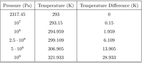
con-stant isRg = 287.06J/(kg K). The barotropic approach is followed since the
temperature difference in the following simulations is negligible (the interested
reader is referred to Appendix B, where the temperature difference in an
isen-tropic compression process is calculated).
400
Differentiating isentropically Eq. (11) with respect to density, constant speed
of sound for the liquid and mixture is found for water: cl = 1482.35m/sand
cm= 1m/s, following Brennen [114] and ¨Orley et al. [107]. For the ideal gas,
the speed of sound is calculated from:
cg=
p
RgTref, (13)
where the specific heat ratio γ = Cp
Cv is unity (isothermal approach). In the
three phase mixture, the speed of sound betweenlmandgphases is determined by the Wallis speed of sound [114, 117]:
1
ρc2 =
1−βg
ρlmc2lm
+ βg
ρgc2g
, (14)
In order to calculate the pressure of the mixture, a closed form equation of state
405
describing the co-existence of three phases is employed from Eq. (6):
ρ=βlm
h
ρl,sat+
1
c2(p−psat)
i
+βg
p RgTref
, (15) replacing the volume fractionβg from Eq. (7) and eliminatingβlmby using Eq.
(9) and Eq. (12), a quadratic equation for the pressure is derived:
where
A= 1
c2, (17)
B =ρ(Yg−1) +ρl,sat−
p c2 −
YgρRgTref
c2 , (18)
C=YgρRgTref
p
sat
c2 −ρl,sat
. (19)
In the case of two real solutions p1, p2 ∈R, the largest root of Eq. (16) is 410
kept. The speed of sound in Eq. (17), (18) and (19) is set to either cl or cm,
depending on the pressure at the previous time step for identifying the liquid or
mixture regions. Therefore, Eq. (16) is solved iteratively, in case the computed
pressure does not fulfil the original assumption. In practice, the algorithm is
repeated for no more than three iterations.
415
3.4. Discretization
Due to the large variation in the speed of sound, the Mach number in three
phase flows can range from 10−2 up to 102 or even higher [118]. As it can be seen in the previous sub-section from Eq. (13) and (11), the speed of sound
can vary from 1m/s in the mixture regime, up to 1482.35m/s in the liquid
420
region, whereas in the gaseous phase the speed of sound is 290m/s. This is an obstacle in density-based solvers, since they are prone to slow convergence and
dispersion in low Mach number flows [119, 120, 121]. In order to handle the low
Mach number problem, a hybrid flux, suitable for multiphase flows, is proposed
here for first time.
425
The aforementioned flux is based on the Primitive Variable Riemann Solver
(PVRS) [122] and the Mach consistent numerical flux of Schmidt et al. [123].
That way, an efficient and robust solver is developed, by utilizing an
scheme is suitable for subsonic up to supersonic flow conditions. The numerical
430
inviscid flux in thekdirection at thei+ 1/2 interface takes the following form:
Fi+1/2k =ρL/Ru?k
1
YgL/R
uL/R1 uL/R2 uL/R3
+p?
0 0 δ1k δ2k δ3k , (20)
where the interface velocityu?
k is approximated by:
u?k = 1
CL+CR[C LuL
k +C RuR
k + (p
L−pR)], (21)
andCis the acoustic impedance C=ρc. The interface pressurep? is:
p?= (1−β)p?,incr+βp?,comp. (22) In Eq. (22), the interface pressure is the sum of the incompressible and the
compressible parts, where the incompressible contribution is:
435
p?,incr= C
LpR+CRpL
CL+CR , (23)
and the compressible contribution is:
p?,comp=C
LpR+CRpL+CRCL(uL k −uRk)
CL+CR (24)
Depending on the Mach number, the contribution of the incompressible or the
compressible part in Eq. (22) is more dominant and the weighted termβ is :
β = 1−e−αM, (25) where the Mach numberM is defined as:
M =max|u
L|
cL ,
|uR|
cR
The blending coefficient is α∼(10,100). For incompressible single phase flow,
440
Eq. (23) is taking the form of 12(pL+pR) since CL =CR. However, for
two-phase flows, Eq. (23) is much closer to the exact solution.
Linear interpolation (2nd order spatial accuracy) with van Leer flux limiter
has been used [124]. A four stage Runge-Kutta (RK), 4th order accurate in
time has been implemented for time advancement [122], in order to capture the
445
waves which are propagating in the domain.
4. Results
In this section, verification and validation of the numerical method is
per-formed; then, the effect of various impact velocities on a 2-D axisymmetric drop
impact is investigated. The Riemann problem is chosen for verifying the
algo-450
rithm accuracy and demonstrating its ability to resolve wave dynamics. Possible
difficulties of the numerical scheme, which is prone to numerical diffusion and
dispersion, especially at the phase boundaries are also investigated. The 2-D
planar drop impact case is then selected for qualitative validation of the
prop-agating shock and the reflected expansion waves against available experimental
455
data. Finally, the 2-D axisymmetric drop impingement on a solid wall is
mod-elled for different impact velocities, in order to investigate the extent of the
cavitation zone and how bubble collapse can possibly lead to material erosion.
The drop impact simulations are summarised in Table 1, where the Reynolds,
Weber and Froude numbers are calculated.
460
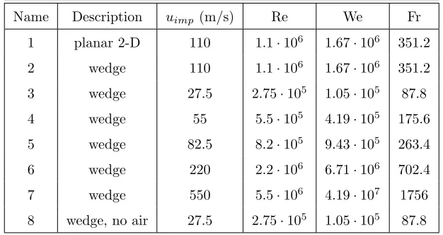
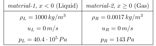
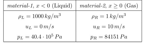
4.1. Riemann Problem
The first benchmark case is the Riemann problem in the computational
do-mainx∈[−0.5,0.5] with initial conditions for the left state: ρL = 998.2kg/m3,
uL = 0m/s, Yg = 0 and for the right state: ρR = 0.017kg/m3, uR = 0m/s,
Yg = 1. Wave transmissive boundary conditions have been used for the left
465
and the right sides of the shock tube, that isUn+1(x=L) =Un(x=L) and
Table 1: Numbering, description, impact velocity, Reynolds, Weber and Froude numbers of
the drop impact cases which have been simulated. As wedge are denoted the 2-D axisymmetric
simulations and no air means that in the initial condition the drop is attached to the wall,
in comparison to the rest of the simulations where the drop is 3 cells above the wall in the
beginning of the simulation.
Name Description uimp(m/s) Re We Fr
1 planar 2-D 110 1.1·106 1.67·106 351.2 2 wedge 110 1.1·106 1.67·106 351.2
3 wedge 27.5 2.75·105 1.05·105 87.8
4 wedge 55 5.5·105 4.19·105 175.6
5 wedge 82.5 8.2·105 9.43·105 263.4
6 wedge 220 2.2·106 6.71·106 702.4
7 wedge 550 5.5·106 4.19·107 1756
8 wedge, no air 27.5 2.75·105 1.05·105 87.8
step selection in the explicit algorithm. Comparison between the exact and the
numerical solution is shown in Fig. 1 at timet= 0.1µs, where second order of spatial accuracy with 500 equally spaced cells in the x direction was used for
470
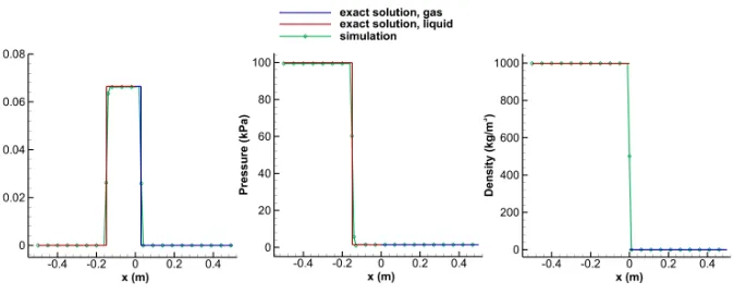
obtaining the numerical solution. A close-up view in order to compare first and
second order in space schemes with resolution either 500 or 1000 equally spaced
cells in the x direction is shown in Fig. 2. In Fig. 1, the exact solution of the
Riemann problem and the computed one are in satisfactory agreement and the
wave pattern has been correctly captured. As it was expected in Fig. 2, the 2nd
475
order solutions in space have minimal numerical diffusion, which is dominant
in the 1st order schemes. In addition, the computed solution is getting closer
to the exact by increasing the mesh resolution and the numerical diffusion is
eliminated. No dispersion is noticed at the boundary interface (between the
gas and the liquid), which is the case when using conventional schemes such as
480
HLLC or similar. The exact solution of the Riemann problem is not trivial for
multi-material cases and it has been derived following the Appendix A of the
Figure 1: Verification of the two-phase solver in the Riemann problem. Comparison of the
x-velocity (left), pressure (middle) and density (right) between the exact and the numerical
solution at timet= 0.1 µs. Second order accuracy in space with 500 cells has been used.
4.2. Planar drop impact
The second test case examined is a planar ’drop’ impact on a solid wall for
485
which experimental data are available [12]. A 2-D simulation, with second order
discretization in space has been performed in order to validate the algorithm
against the 2-D experimental data of Field at al. [12]. In the experimental
apparatus of [12], a small quantity of liquid was placed between two transparent
plates, separated by a small distance. Due to surface tension, the liquid formed
490
a circular area of diameterD= 10mm; the distance between the two plates is negligible compared to the diameterD. The impact was modelled by a third plate which was projected with velocity 110m/samong the two plates. In the numerical simulation, the water drop (Y = 0) and the surrounding air (Y = 1) were set as initial conditions in the transport equation for the gas mass fraction.
495
Therefore, the centre of the drop was placed at (x0, y0) = (0,0.00505)min the
computational domain (−0.2,0.2)×(0,0.2)m; 150 cells have been placed along the initial drop radiusR (grid size∼33µm). The same cell size as in the drop radius has been kept until distance 2R in the positive and negative x-direction and until 1.5Rin the positive y-direction. After that, a stretching ratio of 1.05
500
Figure 2: Close-up view of the Riemann problem. Comparison of the x-velocity (left) and
pressure (right) between the exact and the numerical solution at timet= 0.1µs. First and
second order spatial accuracy schemes with resolution of 500 and 1000 cells have been used.
5·10−9s) in the explicit algorithm. Initially, the pressure of the surrounding
air and the water drop is atmospheric,p(t= 0) = 101326P a. In this way, the initial density for the two phases is calculated from the barotropic EoS:ρl(t=
505
0) = 998.207kg/m3 and ρg(t = 0) = 1.204kg/m3. Zero gradient boundary
conditions have been selected for the right, left and upper faces, whereas the
lower face is set as wall. In Fig. 4 the experiment [12] (left) and the numerical
[image:24.612.143.475.493.610.2]solution (right) for the drop impact are compared.
Figure 3: Computational grids for the planer drop impact (left) and for the 2-D axisymmetric
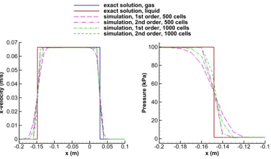
The main mechanisms noticed both in the experimental work [10, 12] and
510
past numerical simulations [102, 104, 105] are jetting, as well as shock and
expan-sion waves; these are also identified in the present study. In the aforementioned
compressible numerical studies, cavitation was not modelled and different
im-pact conditions were simulated compared to the present work. In frame(a)the
drop impacts the wall, whereas in the next frame, a shock wave is forming, as a
515
result of the impact. While the liquid close to the impact point is compressed,
the information of the impact has not travelled in the rest of the drop, which is
still moving with the impact velocity [100]. Those two regions are separated by
the shock front (frame(b)), which is created by individual wavelets emanating
from the contact edge [101, 10]. In the preliminary stages of the impact, the
520
edge velocity is higher than the speed of sound and there is a tendency to
de-crease. As long as the edge velocity is higher than the shock speed, the shock is
attached to the contact edge. When the edge velocity reaches the critical value
of the shock speed, the shock wave is detached from the contact line (frame(c))
and it is propagating in the rest of the liquid (until frame(g)). This mechanism
525
is responsible for the expansion of the liquid and the jetting, which is created
in the contact edge (frame (d), denoted as J in the experimental results). In
frames(e), (f ) and (g), the shock wave is reflected normal to the free surface
as an expansion wave which focuses in the inner region of the drop. These low
pressure areas are potential cavitation regimes and their extent, as well as the
530
volume of the vapour depend on the impact velocity [105]. In frames(g), (h),
the shock wave reaches the highest point of the drop and it is then reflected
downwards. In the last frames, the jetting is more advanced and the reflected
shock is shown in the upper middle of the drop at frames(i) and(j) (denoted
as R in frame(i) and focused to point F in frame(j) of the experiment).
535
Comparing the present simulation with previous experimental studies of
Field et al. [12], similar wave structures at the same time scale are noticed.
The edge pressure in the contact edge is around 0.22GP a and it exceeds the water hammer pressure [10], which is estimated about 0.16GP a, where the wa-ter hammer pressure is defined as pwh = ρlcluimp. The shock wave moving
upwards and its reflection have been recognized at similar time frames between
the experiment and the simulation. Furthermore, the jetting (starting from
frame (d)) is around ten times the impact speed, or even higher, as it has
been mentioned in [10]. Rarefaction waves have been also identified in the later
stages of the drop impact and they follow the same pattern as in the
experi-545
mental study. The production of vapour in the final stages is evident due to
the pressure drop and the areas where vapour is generated are in accordance
to the experiment. However, in the experimental study the maximum volume
of vapour is in the centre of the drop, whereas in the present work, vapour is
more dominant on the upper sides, perimetrically of the drop. This is because
550
[image:26.612.134.482.325.615.2]the bulk liquid tension cannot be captured with the present methodology.
Figure 4: Validation of the numerical solution (right) against experiment (left) for a 2-D drop
impact on a solid wall with impact velocity 110m/s. The interframe time ist= 1µs. The
4.3. 2-D axisymmetric drop impact
The previous simulation is now performed in a 2-D axisymmetric
compu-tational domain, in order to model the impact of spherical drops. A 3-D
sim-ulation would generally capture the 3-D interfacial instabilities due to surface
555
tension, but since the We number is above 105 and in order to reduce the
com-putational cost, a 2-D axisymmetric simulation is performed instead. The drop
impact time scale istimpact =D/uimp and in the present configuration for
im-pact velocity uimp = 110m/s is calculated to betimpact ≈9·10−5s, whereas
the cavitation collapse time is approximated from the characteristic Rayleigh
560
timetcav = 0.915R0,vap
q ρ
l
p∞−psat and it is calculated to betcav≈2.2·10
−5s.
Starting from the half of the 2-D meshes of 4.2, a wedge of 5 degrees has been
simulated by taking advantage of the axial symmetry (see the right image of
Fig. 3). The same initial and boundary conditions are kept, apart from the
wedge faces and the axis of symmetry. At the beginning, a grid independence
565
analysis is performed and then, the effect of the impact velocity magnitude is
investigated for the intermediate grid. Second order accurate spatial
discretiza-tion schemes have been used for this simuladiscretiza-tion and a CFL number of 0.5 was chosen for the time step selection (∆t ∼3·10−10s) in the explicit algorithm.
In the following figures, pressure has been non-dimensionalized with the water
570
hammer pressurepwh, velocity with the impact velocity uimp and the
dimen-sionless time is calculated from: t = T−tbimp
D/cl , where tbimp = 0.00005/uimp is
the time of the impact, based on the initial configuration (in cases where the
drop is not attached to the wall, but there is air between them). This way, the
shock wave will be at the same y-position at a given non-dimensional time for
575
all impact velocities.
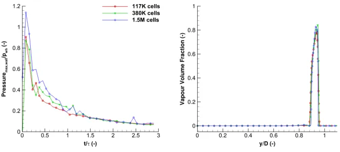
In Fig. 5 the results of the grid independence study are shown, for an impact
velocity of 110m/s. Three different grids have been utilized, with 117k, 380k
and 1.5M cells. In the fine area: (0,2R)×(0,1.5R) the resolution of 330×225, 660×450 and 1320×900 cells has been used for the three different grids. On
580
the left-hand side of Fig. 5, the maximum wall pressure with respect to time
parallel to the y axis (x= 0.6mm) at timet= 1.19 is plotted. The maximum wall pressures are similar for all grids and the peak noticed in the vapour volume
fraction aftery= 0.8 is almost identical for all resolutions. It can be concluded
585
from the above study that there is convergence of the solution for the selected
grid resolutions. The intermediate grid (380k cells), referred as case 2 from now on, is considered to be accurate enough and it is selected for the rest of the
simulations.
In Fig. 6 and 7 the evolution of the drop impact is shown forcase 2. More
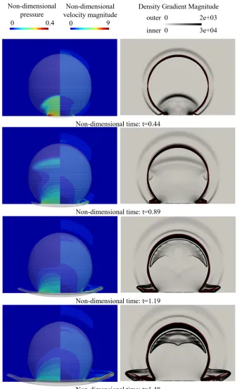
590
specifically, in Fig. 6 the pressure field (left half) and the velocity magnitude
(right half) are shown in conjunction with the iso-surface of 0.5 gas mass frac-tion on the left figures; whereas on the right figures, the numerical Schlieren is
depicted by utilizing different scales for the inner and the outer computational
domain of the drop in order to capture the different waves, which are
propagat-595
ing in the liquid water and in the air. In Fig. 7 the wall pressure (lower part)
and the vapour volume fraction (upper part) combined with the iso-surface of
0.5 gas mass fraction are demonstrated for case 2. The main mechanisms and the flow pattern in the 2-D axisymmetric simulation (case 2) are similar to the
planar one (case 1) for the same impact velocity (110m/s). At timet = 0.44
600
the drop has already impacted the wall and the shock wave is visible in the
Schlieren figure. The jetting has started, however it is more evident at time
t= 0.89 and it is responsible for the non-spherical shape of the drop. As the shock moves to the upper half of the drop, it is reflected on the drop surface
and expansion waves, which are moving downwards, are noticed in the Schlieren
605
figures, starting from timet= 0.89. Those rarefaction waves create low pressure areas and thus, cavitation is noticed at timest = 1.19 and t = 1.48 (see also Fig. 7). The maximum wall pressure is realised at the moment of the impact
and it decreases afterwards (see Fig. 12).
The planar and the axisymmetric solutions exhibit many similarities;
never-610
theless, there is a discrepancy in the pressure field betweencase 1 andcase 2.
The maximum wall pressure is higher incase 1, as it can be seen in Fig. 8 and
propa-gates in a cylindrical pattern and it is reflected on the upper half surface of the
cylinder, whereas incase 2 the shock wave travels in a spherical pattern and it
615
is reflected on the upper surface of the spherical drop. The three-dimensionality
of the latter results in a shock wave of the half pressure strength (∼10M P a), compared to the planar case (∼20M P a).
In Fig. 9, the above results are compared to lower impact velocities, 55m/s
and 27.5m/sat the same dimensionless timet= 1.48. The same configuration
620
as in the left image of Fig. 6 is followed here as well. The drop spreading at
lower impact speeds is less dominant and the drop is closer to the spherical
shape, as it can be seen from the drop iso-surface plots. On the other hand, in
case 2 the transition to splashing is evident, as the jetting area is split to two
different regions. Furthermore, the high pressure area and the lamella are larger
625
in case 2 but the ratio|umax|/uimp in all cases (case 2-4) is between 7.2 and
11, whereas the ratio pmax/pwh is around 0.13. Although the above indicate
similar non-dimensional maximum pressures and jetting velocities regardless the
impact velocity, it is worth pointing out that the maximum pressure and velocity
fields are significantly lower incase 3 and4. For example, the jetting velocity
630
is reduced by even one order of magnitude (∼1400m/sincase 2 and∼190m/s
incase 4 ).
In order to compare the vapour generated for each impact velocity at the
same non dimensional time t = 1.48, slices with the vapour volume contour (upper) combined with the same iso-surface are shown in Fig. 10 forcase 2, 3
635
and4. For the highest impact velocity (case 2) the vapour volume is increased
even one order of magnitude compared to the values of lower velocities. It can
be concluded that the amount of the vapour and the extent of the cavitation
area, which is generated at later stages, monotonically depends on the impact
velocity (this is also evident in Fig. 12 where 6 different impact velocities are
640
examined). The wall pressure (bottom) is also depicted in Fig. 10; although the
maximum is approximately the same for all cases, it extends to a larger area for
higher impact velocities.
than at timet= 1.48. In Fig. 11 the pressure field (left slice) and the velocity
645
magnitude (right slice) are shown in conjunction with the iso-surface of 0.5 gas mass fraction on the left figures, whereas on the right figures the wall pressure
(lower slice) and the vapour volume fraction (upper slice) combined with the
iso-surface of 0.5 gas mass fraction are demonstrated forcase 2. Several vaporous regions have been created from the rarefaction waves and they start collapsing
650
consecutively. At timest = 3.19 and t = 3.56 the third and second vaporous regions have just collapsed respectively. A peak in the pressure due to the shock
wave created by the collapse is noticed at timest= 3.56 andt= 3.64, however the location (far away from the wall) and the strength (maximum pressure is
0.09pwh) cannot denote erosion.
655
In Fig. 12 a parametric study for six different impact velocities (case
2-7) is performed for the intermediate grid resolution, where the maximum wall
pressure (left) and the generated volume of vapour (right) with respect to time
are plotted. As it has been already discussed in the previous paragraph and
in previous studies [7, 105], it is straightforward that higher impact velocities
660
result in higher wall pressures (although the ratio pmax,wall
pwh is almost constant
regardless of the impact velocity). More production of vapour due to the
reflec-tion of a stronger shock developing during the liquid-solid contact is calculated.
The cavitation inside the drop may also contribute to pressure increase on the
solid surface at the bubble collapse stage. This is shown on the wall pressure
665
figure, where at higher impact velocities there are small peaks occurring at later
times (case 7).
It is remarkable that the initial configuration can affect the existence or not of
cavitation and material erosion close to the wall, even for low impact velocities.
As initial condition incase 8 is now selected the drop to be attached to the wall
670
(in contrast tocase 1-7), so there is no air between them. To demonstrate that
the impact velocity is not the determining factor here, uimp = 27.5m/s was
selected. Surprisingly enough, in Fig. 13 vapour is created at the impact point
and a vaporous region is formed above it due to a rarefaction wave at an early
stage of the impact. The maximum vapour volume fraction created is even three
times higher than case 2 at timet = 1.48, where the impact velocity is four times larger. Consequently, there is a significant increase in the pressure field
due to the collapse, as it can be observed in Fig. 14, which results in around
60% higher wall pressure, compared tocase 3. In practice, the above case can
be realised at steam turbine blades, where the rarefied environment implies very
680
[image:31.612.140.472.251.400.2]low steam density, consequently there is little drop/vapour interaction.
Figure 5: Grid independence study for three different grids (coarse, intermediate, fine).
Max-imum wall pressure with respect to time is shown on the left. The values of the vapour
volume fraction on the right figure are exported at a line parallel to the y axis starting from
x= 0.6mm, z= 0 at timeT= 0.083. Wall pressure is divided bypwh, time is measured from
the moment of the impact and it is non-dimensionalized withτ =D/cl, whereas distancey
has been divided by the drop diameterD.
5. Conclusions
In the present work, the impact of drops onto solid surfaces at conditions
inducing cavitation within its volume have been addressed. Initially, a
litera-ture review on the subject has been given, focusing primarily on computational
685
studies. It is apparent that the vast majority of them assume incompressible
liquids and aim to resolve the temporal development of the drop/gas interface.
Studies that consider the heat transfer and phase-change phenomena induced
not been addressed here. However, more relevant to the present study are the
690
conditions at high impact velocities where liquid compressibility becomes
im-portant. For conditions inducing cavitation within the drop’s volume, only one
set of experiments is reported in the literature while no computational study has
been performed so far. Aiming to provide further inside to this problem, an
ex-plicit density-based solver of the Euler equations, able to model the co-existence
695
of non-condensable gases, liquid and vapour phases has been developed and
im-plemented in OpenFOAM. Moreover, a Mach number consistent numerical flux,
capable of handling a wide range of Mach number flows and producing smooth
solutions at the phase boundaries has been proposed. The main model
assump-tions and simplificaassump-tions have been justified for the flow condiassump-tions of interest
700
to the present study. The developed algorithm was then validated against the
Riemann problem, followed by the comparison against the 2-D planar ’drop’
im-pact experiment, showing satisfactory agreement, as similar flow patterns have
been identified. Following, simulation of the impact of spherical drops on a
solid surface have been performed, including for the first time the simulation of
705
cavitation formation and collapse. These cavitation regimes are formed by the
reflection of the shock wave on the outer surface of the drop as an expansion
wave.
The drop impact time scale istimpact=D/uimpand in the present
configura-tion for impact velocityuimp= 110m/sis calculated to betimpact≈9·10−5s,
710
whereas the cavitation collapse time is approximated from the characteristic
Rayleigh time tcav = 0.915R0,vap
q ρ
l
p∞−psat and it is calculated to be tcav ≈
2.2·10−5s. The significantly larger time scale (t
impact ≈9·10−5s) of the drop
impact phenomenon in comparison to the characteristic time of the cavitation
collapse (tcav ≈2.2·10−5s) justifies why the collapse of the vaporous regions
715
inside the drop don’t affect the shape of the drop and its splashing. Increased
impact velocity may result in more damage and possibly material erosion not
only because of higher impact pressure, but also due to the collapse of the
va-porous bubbles inside the drop. It is found that the initial location of the drop
with respect to the solid surface, which actually means the absence or not of
gas around the drop, can influence the volume of cavitation generated at the
initial stages of the impact. If there is no gas between the drop and the solid
surface, pressure can get close to its maximum value, which is at the moment
of the impact (pwh) and material erosion may take place (pwh = 160M P afor
uimp = 110m/sand the yield strength of steel is 200−300M P a). It should
725
be clarified here that the above phenomenon can even occur at low impact
velocities, for instance at impact velocityuimp= 27.5m/s.
Acknowledgements
The research leading to these results has received funding from the
MSCA-ITN-ETN of the European Union’s H2020 programme, under REA grant
agree-730
ment n. 642536. The authors would also like to acknowledge the contribution of
The Lloyd’s Register Foundation. Lloyd’s Register Foundation helps to protect
life and property by supporting engineering-related education, public
engage-ment and the application of research.
Appendix A. Exact Riemann problem for multi-material problems
735
In this section, the methodology for finding the exact solution to the
Rie-mann problem for the multi-material Euler equations is derived. In the literature
there are limited works discussing exact Riemann solvers for multi-material
ap-plications. Mainly, these focus on multiple velocities, pressures and temperature
fields, see e.g. [125, 126]. The discussion here will be limited to just two different
740
materials sharing the same velocity, pressure and temperature fields. The
mate-rials will be referred to asmaterial-1 andmaterial-2, however the methodology
may be extended to any number of materials. For the sake of generality, the
discussion will not be limited to an explicit form of equation of state. Instead,
the equations of state for the two distinct materials will be assumed to depend
745
on density and internal energy only, i.e. have a formp=p(ρ) orp= p(ρ, e), which may have an explicit formula or be in tabular form as in [127, 96].
will affect the mixture equation of state. Thus, the mixture equation of state
that will be examined is of the form p=p(ρ, Y) orp=p(ρ, e, Y), where Y is
750
the mass fraction of material-2, defined in Eq. (9). Following Toro [122], the
form of the Riemann problem solved is:
∂U ∂t + ∂F(U)
∂x = 0
U(x,0) =
UL, x<0 UR, x≥0
(A.1)
The same nomenclature as in the rest of the paper is used.
Appendix A.1. Pressure is only a function of density and mass fraction
In case the mixture pressure is only a function of density and mass fraction,
755
p=p(ρ, Y) the conservative variables and the flux vector are:
U= ρ ρu ρY
, F(U) =
ρu
ρu2+p ρuY , (A.2)
To derive the Jacobian matrix, it is convenient to recast theUandF(U) vectors
and equation of statep=p(ρ, Y), as:
U= u1 u2 u3
, F(U) =
u2 u22 u1 +p
u1,uu3
1
u3u2
u1 , (A.3)
p=p
u1,
u3
u1
The Jacobian matrix is calculated as:
A(U) =
∂f1 ∂u1 ∂f1 ∂u2 ∂f1 ∂u3 ∂f2 ∂u1 ∂f2 ∂u2 ∂f2 ∂u3 ∂f3 ∂u1 ∂f3 ∂u2 ∂f3 ∂u3 (A.5)
After calculating all terms and replacing back the conservative variables:
760
A(U) =
0 1 0
∂p ∂ρ−u
2− ∂p ∂Y
Y ρ 2u
1 ρ
∂p ∂Y
−uY Y u
(A.6)
The eigenvalue analysis of the Jacobian matrix results to:
λ1=u−c
λ2=u
λ3=u+c
(A.7)
and right eigenvectors:
K1=
1
u−c
Y
, K2=
∂p ∂Y
u∂Y∂p
Y∂Y∂p −ρ∂p∂ρ
, K3=
1
u+c
Y (A.8)
wherecis the speed of sound equal toq∂p∂ρ. The waves associated withλ1,λ3
eigenvalues are non-linear waves (shock waves or rarefaction waves) and theλ2
eigenvalue is a linearly degenerate wave associated with a contact discontinuity.